Abstract
Wireless sensor networks (WSN) can accurately and timely obtain the production information of crops, and provide data basis for intelligent agriculture. The dynamic crop state and unstable climate environment make it difficult to predict the connectivity probability of wireless links. Therefore, this paper studies an energy-saving opportunity routing transmission strategy under the influence of dynamic link interaction. The protocol establishes an importance model based on algebraic connectivity to reduce the energy consumption of network key nodes. At the same time, based on the improved Bellman–Ford algorithm, a method of constructing candidate sets is studied. It converts the opportunistic routing transmission cost of farm WSN into anycast link cost and the remaining opportunistic path cost affected by energy consumption. The priority queue is used to determine the nodes participating in the iteration, thereby reducing the computational overhead. The protocol also designs a backoff strategy considering the current residual energy to select the only forwarding node and reduce the unnecessary packet copies in the transmission process. Simulation results show that the studied method is superior to the existing opportunistic routing schemes in terms of packet overhead, network lifetime, energy consumption, and packet delivery rate.
1. Introduction
With the development of information technology, modern science is deeply integrated with agricultural production [1]. The Internet of Things (IoT) can remotely sense and transmit farm information, providing basic data for agricultural decision-making. The wireless sensor networks (WSN) are the core of the IoT [2]. It consists of a series of low-cost, low-energy wireless sensors that sense different parameters, including weather, temperature, humidity, and soil moisture. However, the farm has complex terrain, dense crops, a wide geographical area, and sensors that have limited energy and resources. When the data are transmitted to the sink, it consumes energy. Alshehri et al. proposed that the attenuation, reflection, absorption, and scattering on a farm were serious, which may cause the communication link to fail and could not guarantee reliable data transmission [3]. As a farm increases in size, diversity, and complexity, the number of sensors will increase proportionately [4]. The increase in data will cause excessive consumption of network overhead, traffic, and energy [5]. The propagation performance of WSN is deeply affected by the environment. Therefore, designing a routing protocol to optimize the network capacity, energy consumption and network lifetime of agricultural WSN is important.
In an agricultural environment, the dynamic change of wireless links will lead to unreliable communication and affect energy efficiency. The traditional routing protocols obviously do not consider how to deal with the problem of poor link connectivity. Opportunistic routing selects candidate forwarding nodes. These nodes have a chance to become the next hop in the given priority order. Multiple forwarding nodes cooperate to form space diversity, which greatly improves transmission reliability [6]. The current studies on opportunistic routing mainly focus on the minimum transmission cost with little consideration of energy consumption and link interaction.
The main contributions of this paper are as follows:
- This method introduces algebraic connectivity to quantify the importance of the nodes in the farm WSN. When constructing the candidate set, the key nodes are not frequently used, which prolongs the network lifetime.
- Considering the opportunistic forwarding of candidate sets, the transmission cost is transformed into anycast link cost, and the remaining path cost is affected by energy consumption. Design construction rules of the candidate set are based on factors such as node energy consumption, the importance of the node, and distance to sink.
- We adopt the priority queue to calculate the transmission cost iteratively to construct candidate sets. Then, the invalid copies are reduced by defining the backoff time, so the transmission efficiency in WSN is further improved.
2. Related Works
In view of the instability of transmission in the agricultural environment, the research on how to use WSN to effectively transmit agricultural information has attracted many researchers. The energy consumption, transmission delay, and throughput have an important impact on the network lifetime and monitoring quality. Changes in wireless signal strength under different agricultural scenarios were measured by Cama-Pinto [7] and Raheemah [8]. The signal attenuation model of the farmland ZigBee network was established by using a particle swarm optimization algorithm, which provided a reference for building a monitoring network [9]. Different transmission routing will produce different signal attenuation and affect the WSN lifetime. There were many wireless sensor routing algorithms for the agricultural environment [4]. A routing protocol based on a frontward communication area for collecting climate information in the agricultural field was proposed by Khan et al. [10]. Based on the communication radius, the candidate set in the forward communication range was determined. Then, the residual energy was used to select a node to reduce the energy consumption and time delay. The energy centroid was calculated, and nodes close to the energy centroid were regarded as cluster heads [11]. This method balanced the energy consumption and prolonged the network lifetime. However, traditional deterministic routing protocols have many limitations in dealing with unstable links [12]. The studies [13,14,15] showed that opportunistic routing strategies are used more and more widely. It makes full use of the broadcast characteristics and has an obvious advantage over traditional routing in solving unreliable links. Opportunistic routing protocol no longer fixes the next node, but selects many next hops, thereby improving performance such as network throughput.
The commonly used opportunistic routing algorithm calculated the shortest path according to different routing metrics. Biswas et al. designed the EXOR algorithm to construct the candidate sets and sort forwarding order [16]. The neighbor nodes whose expected transmission count (ETX) was less than the source node ETX were added to the candidate set. The smaller the ETX was, the higher the forwarding priority was. A single ETX index is not enough to quantify the network performance, so the opportunistic transmission cost function with multiple influence factors such as distance, energy, and transmission delivery rate is established. In Mao’s research, the routing overhead was converted into three parts: the broadcast cost, the forwarding node selection cost, and the forwarding communication cost [17]. Adjustable and non-adjustable transmission energy models were introduced to calculate the routing cost and selected the optimal candidate sets. Many studies select candidate sets by simultaneously measuring the impact of network energy and transmission distance [18,19,20]. Bangotra et al. adopted Bayesian machine learning to model the candidate nodes selection process as a supervised multi-class non-linear separable problem [18]. Yee et al. further proposed the energy threshold, combined with the maximum and minimum communication range to select the relay node with higher residual energy at different distances [19]. Additionally, an energy-saving opportunity routing protocol based on area density, relative distance, and residual energy was studied to balance energy consumption [21,22,23]. The references [24] further introduce the transmission probability as one of the indicators for constructing candidate sets. In Kandhoul’s research, the next-hop selection was based on the node’s current energy and its predicted message delivery probability [25]. According to the information of transmission probability, energy, and the number of neighbors of neighbor nodes within one hop range, reference [26] updated node weights through reinforcement learning to select candidate sets. In addition, node capacity was also used as an indicator to evaluate the performance of candidate nodes. Ge et al. designed a new hybrid fitness function based on parameters such as energy, trust, QoS, connectivity, distance, hop count, and network traffic, so as to select the best opportunistic routing [27].
In addition, some scholars took geographical location and distance as routing metrics and proposed a routing protocol based on geographic location strategy [28,29,30]. Considering node location, link quality, and node density, a greedy scheme was proposed by Ghaffari et al. [31]. The relay node selected the nearest neighbor to minimize the hops between the source node and the target node. A forwarding decision method was used to select the relay node according to the forwarding probability [32]. Based on the location information, depth information, and current residual energy, Karim et al. weighted the normalized energy, transmission probability, and normalized distance to reduce the energy consumption and improve the network lifetime [33]. Shen et al. proposed an energy-aware geographic routing algorithm, which can manage the residual energy and available energy [34]. In view of the highly dynamic network environment and link cost, Pang et al. selected the neighbor closest to the target as the next forwarder according to the geographical location information of each node, regardless of the topology structure [35].
The above methods did not consider the interaction between links when constructing opportunistic routing. Dubois-Ferriere et al. proposed a least-cost opportunistic routing (LCOR) [36]. By calculating the end-to-end multipath weighted cost, the candidate set is constructed and the forwarding nodes are sorted. LCOR selects an excellent neighbor combination and uses the Bellman–Ford algorithm to obtain forwarding priority. However, in large-scale networks, the Bellman algorithm has a high computational cost. The OAPF algorithm calculated the weighted average of all possible paths from the source node to the sink based on the metric EAX [37]. Gao studied the energy consumption model and made routing decisions based on the duty cycle to balance energy consumption and delay [38]. However, the protocol sums the probability of successful transmission as the probability that at least one node successfully forwards data, and its accuracy is limited.
Compared with the above research, this paper focuses on the contribution of forwarding nodes to the whole network connectivity, aiming to reduce the forwarding times and energy consumption of important nodes to ensure network reliability.
3. Modeling of Wireless Sensor Networks in Farms
As shown in Figure 1, assume that N sensor nodes are deployed in different locations on the farm. The WSN is abstracted as a graph model G = (V, E), where V = {v1, v2, …, vN} denotes N sensors, and E = {e11, e12, …, eij, …, eNN} indicates connectivity between nodes. Because dense crops in the farm will affect the connectivity of link connectivity, we use probability peij as the probability of successful transmission between node i and node j, and the probability of fail transmission is expressed as 1-peij. Let Ee = {Ee1, Ee2, …, EeN} as the set of residual energy. Ne(i) represents the neighbor node set within the communication range of node i. Based on the agricultural WSN model, this paper explores the opportunistic routing affected by energy consumption.
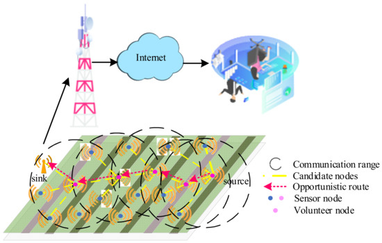
Figure 1.
Schematic diagram of opportunistic routing in farm WSN.
- (1)
- Importance model of nodes
Frequent changes in farmland environment, diverse agricultural operations, and rapid growth of crops make connectivity changes over time, which affect the overall efficiency of routing transmission. The traditional metrics mainly focus on the importance of a single link by predicting link quality or calculating transmission probability without overall consideration of network performance.
The algebraic connectivity reflects the communication possibility. For undirected graph G = (V, E), Laplacian matrix L = D-A can be obtained by adjacency matrix A = (aij) and node degree matrix D = diag({|Ne(1)|, |Ne(2)|, …, |Ne(i)|, …, |Ne(N)|}). If there is a communication link between node i and node j, aij = 1, otherwise aij = 0. |Ne(i)| denotes the node degree of node i. L is a positive semi-definite symmetric matrix, and the second smallest eigenvalue is the algebraic connectivity of G. Algebraic connectivity usually adopts the neighbor node number to measure the connectivity redundancy. However, when the sink position is fixed, node i selects the candidate nodes whose ETX are less than node i, that is, the nodes closer to the sink as the candidate nodes. The link cost is used as the link weight to represent the Laplacian matrix elements of graph G, and the neighbor nodes with ETX less than node i are redefined as Ne(i). This paper establishes the following importance model based on algebraic connectivity [28]:
The second smallest eigenvalue of the matrix L represents the connectivity redundancy of graph G. For graph G (V, E), if delete several links from E to obtain graph G′ (V, E′), λ(G′) ≤ λ(G). Deleting the communication links of node i, and the corresponding algebraic connectivity λi can be obtained. Therefore, the importance model corresponding to node i is defined as λi. The larger the λi, the greater the node’s contribution to the network connection and the more important this node is in maintaining the stable transmission.
- (2)
- Energy consumption model
Every time a node sends or receives data, there will be energy consumption. Exhausting energy may lead to network partition and affect network connectivity and communication quality. This paper uses the first-order energy model to measure energy consumption. The energy consumption of sending k bit data to distance d is as follows [29]:
where Eelec is the energy consumed by the sending module and receiving module to process 1 bit data; εfs and εmp are the energy consumed by power amplification. When the distance between two nodes is less than the threshold (), the free space model is used, otherwise, the multi-path model is adopted. The energy consumption of receiving k bit data are as follows:
3.1. Anycast Transmission Cost
If the probability of successful transmission between node i and node j is peij, the probability that the data sent by node i is received by at least one node in the candidate set Ci is as follows:
According to the importance model, we define the transmission cost as shown below. The more important a node is to maintain the network transmission performance, the higher the transmission cost is:
where λi represents the algebraic connectivity of node i. Additionally, λmax represents the maximum algebraic connectivity in the current network.
One anycast transmission from node i to the candidate set Ci requires Ti broadcasts. Ti is the expected transmission count. The transmission cost of node i broadcasting Ti times is as follows:
3.2. Remaining Opportunistic Path Transmission Cost
For opportunistic routing in WSN, the transmission path is determined according to candidate sets and forwarding priority. Suppose the candidate set of node i is Ci = {ci1, ci2, …, cin}, which has been arranged in ascending order based on the transmission cost CQ1 < CQ2 < … < CQn. If the node ci1 with the highest priority receives the data packet first, then regardless of whether other candidate nodes receive the data packet, ci1 will be regarded as the next hop to forward data.
where, is the probability that data are successfully received from node i to node ci1. α is the weight parameter. If it is not received successfully, the node with the second priority is selected to transmit. If the candidate node ci1~ciu-1 did not receive the packet successfully until the data are received and forwarded by node u, the remaining opportunity routing transmission cost is:
is the probability that the data are sent from node i to ci1~ciu-1 failed and received successfully by ciu.
In opportunistic routing, each forwarding node itself is opportunistic forwarding. If the forwarding priority is determined only by the transmission cost of a single node, there may be a problem that packets are transmitted to bad paths. Considering the interaction between links, this paper takes the transmission cost of the candidate set belonging to the current candidate node as the influencing factor. Therefore, the transmission cost of remaining opportunistic routing is:
The expected transmission cost from node i to sink is the sum of the anycast transmission cost and the remaining opportunistic routing transmission cost :
4. Opportunistic Transmission Strategy for Farm WSN
4.1. Constructing Candidate Set Based on Improved Bellman–Ford
Although the more forwarding nodes, the higher the packet delivery rate, the corresponding transmission cost will increase, which affects the network performance. When the network gain brought by the forwarding nodes is not enough to offset its side effects, the number of forwarding nodes should be controlled. We adopt theBellman–Ford algorithm to calculate the remaining opportunistic routing transmission cost. Firstly, based on the ETX and energy threshold, the EXOR algorithm is used to obtain the initial candidate sets. Then, the initial candidate set is regarded as the neighbor set of node i to obtain the final candidate set by iteration. Then, the transmission cost is calculated when the current node is added to the final candidate set. If the cost is reduced, it is added to the final candidate set. On the contrary, if adding the current candidate node will increase the transmission cost of node i, this node should not be added to the final set.
It is necessary to search the subset of each neighbor set in the iterative process, which has a large algorithm overhead. Therefore, we study the improved Bellman–Ford algorithm to select candidate sets of the farm WSN opportunistic routing. Set A is defined as the set of nodes whose transmission cost becomes smaller in the last iteration and set B is defined as the set of nodes whose transmission cost becomes smaller in this iteration. The improved algorithm for building the candidate set is as follows:
- (1)
- Let CQsink = 0, CQi = +∞, 2 ≤ I ≤ N, and add the sink to set A. Initialize algorithm parameters, h = 1, CQ10 = 0, CQi0 = +∞, 2 ≤ i ≤ N.
- (2)
- In the h-th iteration, the transmission cost of node i in A is calculated. If the neighbor node j joins the candidate set and makes the transmission cost CQjh smaller, node j is added to the candidate set. At the same time, it is judged whether node i belongs to B, if not, node i is added to set B.
- (3)
- When the candidate set of all nodes no longer changes, the algorithm ends, otherwise, the next step is executed.
- (4)
- Empty set A, transfer the elements in set B to set A, and then empty set B. At the same time, for any node i, let CQ10 = CQh0, then let h = h + 1, go to step 2.
| Input: Node number N, node location (xi, yi), and probability peij |
| Output: Candidate set |
| 1.Parameter initialization |
| 2.S = ø; S0 = ø; CQsink = 0; CQi0 = +∞, 1 ≤ i ≤ N; A = {sink}, B = ø, h = 1;3.Initialization of the candidate sets based on ETX |
| 4. for i = 1:N |
| 5. for j = 1:|Ne(vi)| |
| 6. if ETX (j,sink) < ETX (i,sink) and Erth ≤ Erj |
| 7. S0i = S0i ∪ j |
| 8. end if |
| 9. end for |
| 10. end for11. Calculate the minimum expected transmission cost iteratively |
| 12. while CQih = CQih−1 do |
| 13. h = h + 1 |
| 14. for i = 1:N |
| 15. Judge whether there is an intersection between the initial candidate set S0i and set A |
| 16. Store the transmission cost CQh−1 of the neighbor node j in set S0i. and the candi-date set in the h − 1 round |
| 17. if CQ ih < CQih−1 |
| 18. B = B∪i |
| 19. According to the Equation (10), the candidate set and transmission cost of i in round h is calculated. |
| 20. end if |
| 21. end for |
| 22. S = S0, A←B, B = ø |
| 23.end while |
As shown above, the improved Bellman–Ford algorithm and LCOR algorithm have the same algorithm complexity in the worst case, and both are O(nl). However, the improved algorithm in this paper adopts priority queues A and B. The nodes whose transmission cost changes each time are stored in A. In the next iteration, only the transmission costs of other nodes whose candidate set contains B set elements are calculated, which can ensure the quality of candidate set construction and reduce the iteration number, thus reducing the computational overhead.
4.2. Selecting Forwarding Nodes Based on Backoff Time
According to the broadcast characteristics of WSN, the current node can easily send packets to the nodes in the candidate set. However, if a packet is received by many candidate nodes but there is no suitable backoff scheme, these candidate nodes will reply ACK to the source node, which increases the collision possibility and causes unnecessary energy consumption. If the candidate node does not know the data forwarding status of other nodes, there will be multiple copies of the same packet in the network, resulting in invalid throughput.
After the candidate node receives the packet transmitted by the source node, it first executes the backoff time before replying to ACK. This paper defines the backoff time based on the transmission cost:
From the definition of backoff time, the lower the transmission cost is, the higher the forwarding priority is. The node with a smaller transmission cost will have the shortest backoff time. When the backoff time is over, the high-level forwarding node will broadcast the ACK first. In this way, when the source node receives the first ACK message, it knows that its packet has been successfully received. The backoff time of other candidate nodes receiving the packet is longer. If the ACK information from other nodes is received, the source node abandons the received packet and does not forward or reply. Using such backoff and ACK suppression strategies, the opportunity routing protocol of the farm WSN can make the source node unicast data to a candidate node, thereby completing data transmission and reducing the invalid copies in the network.
5. Experiment and Analysis
5.1. Experimental Parameter Setting
This paper verifies the algorithm’s effectiveness through MATLAB. The simulation environment is Intel®Core™ i7-9700U CPU@3.00 GHz with 16 GB RAM. 90~210 nodes are randomly distributed in a farm with a size of 400 × 400 (m2). The sink is in the middle of the farm, and all sensors are isomorphic. Specific experimental parameters are shown in Table 1:

Table 1.
Experimental parameters.
In order to simulate the farm environment, the following channel model is adopted in this paper. Through the path loss model, the link connectivity probability between nodes can be calculated. Additionally, the link instability in the farm is simulated by adding random noise.
This paper compares and analyzes the network performance in four aspects: energy consumption, throughput, delay, and retransmission rate. Reference [19], reference [18], reference [23], and reference [36] are used as comparison algorithms. In this paper, they are represented by Algorithm 1, Algorithm 2, Algorithm 3, and Algorithm 4, respectively.
The network energy consumption (J) is the sum of energy consumed by all nodes until the simulation end. In this paper, it is recorded as EC. The standard energy consumption per package (J/packet) is defined as:
Network throughput is the number of bits of data received by the sink in each round of simulation.
The average delay is the average delay (s) of a data packet from the source node to the sink:
Retransmission rate:
5.2. Analysis of Network Energy Consumption
This paper first verifies the energy performance of five opportunistic routing algorithms based on the number of dead nodes. With the same network topology composed of 90 nodes, the number of nodes that died as time increases is shown in Figure 2. Algorithm 1 mainly calculates the forwarding priority based on the residual energy, so it effectively guarantees the energy consumption balance in the early stage. However, as the number of simulation rounds increases, selecting candidate nodes only depending on the residual energy will lead to some important nodes running out of energy, and the network transmission performance will decline sharply. Algorithm 2 and Algorithm 3 select forwarding nodes by combining residual energy and distance between nodes and sink. No adaptive weights are designed to balance different influencing factors. When the energy gap is not obvious, the nodes with better transmission performance will be frequently used to transmit data. At the same time, because the transmission cost of the candidate set is not considered, the network performance will decline rapidly. Our algorithm and LCOR algorithm construct the candidate set by calculating the path cost, which can effectively avoid invalid transmission to a certain extent. Our algorithm considers both the impact of important nodes on the network connectivity and the impact of residual energy, so the network energy consumption can be evenly distributed to the neighbor nodes, reducing the number of dead nodes.
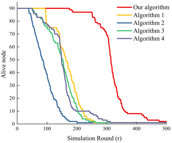
Figure 2.
The number of failed nodes.
In WSN with different numbers of nodes, it can be seen from Figure 3 that the standard energy consumption per package of the studied algorithm is significantly lower than that of the other four algorithms. This means that our opportunistic routing algorithm can still transmit data with low energy consumption under different network topologies.
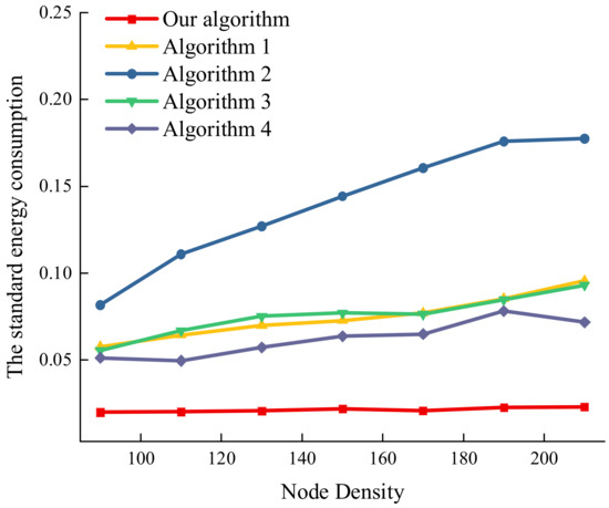
Figure 3.
Network energy efficiency under a different number of nodes.
5.3. Analysis of Network Throughput
When the network topology is fixed, as the number of simulation rounds changes, the change in throughput is shown in Figure 4. The number of dead nodes increases and the link connectivity decreases, which has an impact on the reliable data transmission and the end-to-end throughput. The throughput obtained by the five algorithms all shows a downward trend. However, our algorithm reduces the energy consumption of the important nodes and considers the transmission cost of the interaction between links, which increases the data transmission reliability. This algorithm has higher network throughput.
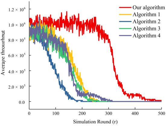
Figure 4.
Throughput of sink.
Then, we change the number of nodes and make them randomly distributed in the farm to obtain normalized throughput under different network topologies, as shown in Figure 5. Due to high energy utilization and slow node death rate, the algorithm has good performance in throughput. This means that our algorithm can monitor and transmit multi-source farm data.
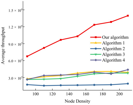
Figure 5.
Network throughput under a different number of nodes.
5.4. Analysis of End-to-End Delay
Figure 6 shows the difference between the four comparison algorithms minus the end-to-end average delay of our algorithm. As the number of dead nodes increases, the communication will be severely affected, and the delay will increase. However, the difference shows that the studied algorithm has obvious advantages over the other algorithms, which can reduce the delay while maintaining a large throughput. In combination with the throughput, the number of packets received by the sink in other algorithms decreases rapidly in late simulation, so the four algorithms have a shorter delay. When the number of simulation rounds is greater than 300 rounds, the nodes of the comparison algorithm almost all die and no longer perform data transmission, so the delay difference does not exist.
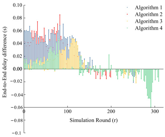
Figure 6.
End-to-End delay difference.
From the Figure 7, we can see that the box shape of our algorithm is the flattest, and Algorithm 2 has the longest box shape. This means that the average delay obtained by this algorithm is stable and can maintain a good average delay for a long period. Since Algorithm 4 considers the remaining opportunistic path transmission cost when constructing candidate sets, it also has a stable delay performance. However, the mean and median of the delay in this algorithm are smaller than that of the other algorithms.
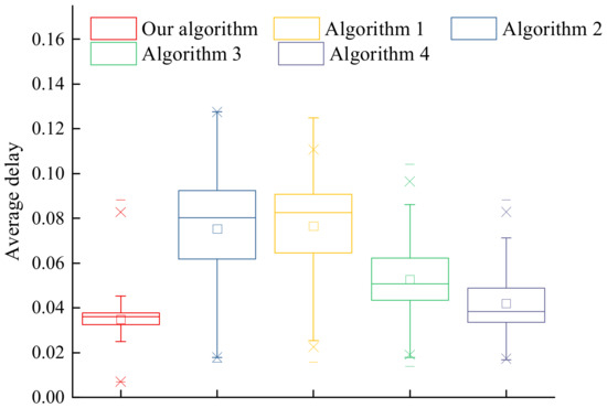
Figure 7.
Box graph of end-to-end delay.
Figure 8 shows the average delay with a different number of nodes. The changing trend of the average delay under the different number of nodes is also consistent with the changing trend of that in a simulation round, which shows our algorithm also maintains a relatively stable delay with different network structures.
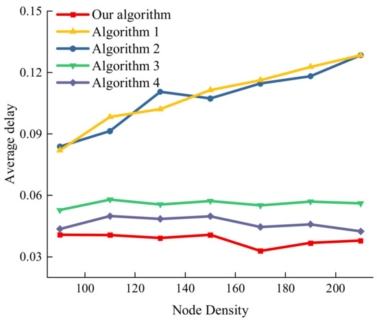
Figure 8.
End-to-end average delay with a different number of nodes.
5.5. Retransmission Rate Analysis
As the number of dead nodes increases, the retransmission rates of the five opportunistic routing algorithms all increase. Figure 9 shows the difference between the four comparison algorithms minus the retransmission rate of the algorithm in this paper. This algorithm considers the influence of nodes on network connectivity. The opportunistic routing not only focuses on the quality of the current forwarding path but also considers the long-term transmission quality of the network.
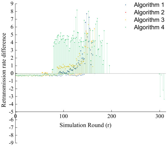
Figure 9.
Retransmission rate difference.
It can be seen from Figure 10 that the median retransmission rate of our algorithm is low, which means that the retransmission times are relatively stable in the whole simulation cycle. At the same time, the median is low, so in the early stage network with sufficient energy, efficient data transmission can be realized. As shown in Figure 11, this algorithm has a low retransmission rate under the different number of nodes.
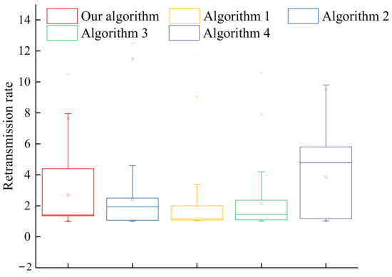
Figure 10.
Box graph of RR.
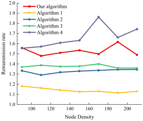
Figure 11.
Retransmission rate under a different number of nodes.
6. Conclusions
Focusing on the actual demand of precision agriculture for wireless sensors, this paper studies an energy-saving opportunistic routing transmission protocol for farm WSN. This paper introduces algebraic connectivity to establish an importance model. On this basis, combined with energy consumption, a transmission cost model combining anycast transmission cost and candidate set path cost is designed. Then, we improved the Bellman–Ford algorithm to calculate the minimum expected transmission cost. The backoff time is studied to sort the forwarding nodes and reduce the number of invalid copies in the network. The simulation experiment results show that the opportunistic routing algorithm studied in this paper has obvious advantages in energy efficiency, throughput, network delay, and packet delivery rate.
Focusing on the actual demand of precision agriculture for wireless sensors, this paper studies an energy-saving opportunistic routing transmission protocol for farm WSN. Opportunistic routing makes use of the characteristics of network broadcast and selects candidate forwarding sets for data transmission to ensure reliable data transmission when links are unstable and connected in the complex environment of the farm. The node importance model is designed based on algebraic connectivity. Combined with energy balance, link interaction, and energy consumption, the opportunistic transmission cost function is constructed. The Bellman–Ford algorithm is improved to calculate the expected minimum transmission cost. Considering the factors of data transmission and network demand, a node forwarding strategy based on backoff time is developed, which can reduce the number of copies in the network while selecting the only forwarding node, and further reduce the network energy consumption. Compared with the comparison algorithms, this algorithm can reduce the energy consumption speed of important nodes and construct a more appropriate candidate set according to the link interaction. Simulation results show that this algorithm can improve packet delivery rate and throughput while limiting network overhead and reducing transmission delay.
This paper mainly studies the opportunistic routing transmission mechanism of static nodes in the farm, but the farm WSN also includes mobile sensing nodes such as UAVs and tractors. Therefore, our further research will mainly focus on the data machine transmission mechanism in the hybrid network where mobile nodes and static nodes exist at the same time.
Author Contributions
Conceptualization, H.W. and X.H.; literature search, figures, table X.H., C.C. and B.Y.; methodology, H.W. and H.Z.; validation, H.Z. and X.H.; formal analysis, X.H., H.Z. and C.C.; writing—original draft preparation, all authors; funding acquisition, H.W. All authors have read and agreed to the published version of the manuscript.
Funding
This research was funded by the National Natural Science Foundation of China, grant number 61871041, and China Agriculture Research System of MOF and MARA, grant number CARS-23-D07.
Conflicts of Interest
The authors declare no conflict of interest.
References
- Tang, Y.; Dananjayan, S.; Hou, C.J.; Guo, Q.W.; Luo, S.M.; He, Y. A survey on the 5G network and its impact on agriculture: Challenges and opportunities. Comput. Electron. Agric. 2021, 180, 105895. [Google Scholar] [CrossRef]
- Sanjeevi, P.; Prasanna, S.; Siva Kumar, B.; Gunasekaran, G.; Alagiri, I.; Vijay Anand, R. Precision agriculture and farming using Internet of Things based on wireless sensor network. Trans. Emerg. Telecommun. 2020, 31, e3978. [Google Scholar] [CrossRef]
- Alshehri, A.; Badawy, A.H.A.; Huang, H. FQ-AGO: Fuzzy Logic Q-Learning Based Asymmetric Link Aware and Geographic Opportunistic Routing Scheme for MANETs. Electronics 2020, 9, 576. [Google Scholar] [CrossRef] [Green Version]
- Mahajan, H.B.; Badarla, A.; Junnarkar, A.A. CL-IoT: Cross-layer Internet of Things protocol for intelligent manufacturing of smart farming. J. Ambient. Intell. Humaniz. Comput. 2021, 12, 7777–7791. [Google Scholar] [CrossRef]
- Mohanty, S.N.; Lydia, E.L.; Elhoseny, M.; Al Otaibi, M.M.G.; Shankar, K. Deep Learning with LSTM Based Distributed Data Mining Model for Energy Efficient Wireless Sensor Networks. Phys. Commun. 2020, 40, 101097. [Google Scholar] [CrossRef]
- Geng, H.J.; Shi, X.G.; Yin, X.; Wang, Z.L.; Yin, S.P. Algebra and Algorithms for Multipath QoS Routing in Link State Networks. J. Commun. Netw. 2017, 19, 189–200. [Google Scholar] [CrossRef]
- Cama-Pinto, D.; Damas, M.; Holgado-Terriza, J.A.; Gomez-Mula, F.; Cama-Pinto, A. Path loss determination using linear and cubic regression inside a classic tomato greenhouse. Int. J. Environ. Res. Public Health 2019, 16, 1744. [Google Scholar] [CrossRef] [Green Version]
- Raheemah, A.; Sabri, N.; Salim, M.S.; Ehkan, P.; Ahmad, R.B. New empirical path loss model for wireless sensor networks in mango greenhouses. Comput. Electron. Agric. 2016, 127, 553–560. [Google Scholar] [CrossRef]
- Wang, T.; Zeng, J.D.; Lai, Y.X.; Cai, Y.Q.; Tian, H.; Chen, Y.H.; Wang, B.W. Data collection from WSNs to the cloud based on mobile Fog elements. Future Gener. Comput. Syst. 2020, 105, 864–872. [Google Scholar] [CrossRef]
- Khan, T.H.F.; Kumar, D.S. Ambient crop field monitoring for improving context based agricultural by mobile sink in WSN. J. Ambient. Intell. Humaniz. Comput. 2020, 11, 1431–1439. [Google Scholar] [CrossRef]
- Qureshi, K.N.; Bashir, M.U.; Lloret, J.; Leon, A. Optimized cluster-based dynamic energy-aware routing protocol for wireless sensor networks in agriculture precision. Sens. Appl. Agric. Environ. Monit. 2020, 2020, 9040395. [Google Scholar] [CrossRef] [Green Version]
- Hsu, C.J.; Liu, H.I.; Seah, W.K.G. Opportunistic routing—A review and the challenges ahead. Comput. Netw. 2011, 55, 3592–3603. [Google Scholar] [CrossRef]
- Guan, Q.S.; Ji, F.; Liu, Y.; Yu, H.; Chen, W.Q. Distance-vector-based opportunistic routing for underwater acoustic sensor networks. IEEE Internet Things J. 2019, 6, 3831–3839. [Google Scholar] [CrossRef]
- Yousofi, A.; Sabaei, M.; Hosseinzadeh, M. Design of optimum criterion for opportunistic multi-hop routing in cognitive radio networks. ETRI J. 2018, 40, 613–623. [Google Scholar] [CrossRef]
- Biswas, S.; Morris, R. ExOR: Opportunistic multi-hop routing for wireless networks. In Proceedings of the 2005 Conference on Applications, Technologies, Architectures, and Protocols for Computer Communications, Philadelphia, PA, USA, 22–26 August 2005. [Google Scholar]
- Kashani, A.A.; Ghanbari, M.; Rahmani, A.M. Improving the performance of opportunistic routing protocol using the evidence theory for VANETs in highways. IET Commun. 2019, 13, 3360–3368. [Google Scholar] [CrossRef]
- Mao, X.F.; Tang, S.J.; Xu, X.H.; Li, X.Y.; Ma, H.D. Energy-efficient opportunistic routing in wireless sensor networks. IEEE Trans. Parallel Distrib. Syst. 2011, 22, 1934–1942. [Google Scholar] [CrossRef] [Green Version]
- Bangotra, D.K.; Singh, Y.; Selwal, A.; Kumar, N.; Singh, P.K.; Hong, W.C. An intelligent opportunistic routing algorithm for wireless sensor networks and its application towards e-Healthcare. Sensors 2020, 20, 3887. [Google Scholar] [CrossRef]
- Yee, P.L.; Mehmood, S.; Almogren, A.; Ali, I.; Anisi, M.H. Improving the performance of opportunistic routing using min-max range and optimum energy level for relay node selection in wireless sensor networks. PeerJ Comput. Sci. 2020, 6, e326. [Google Scholar] [CrossRef]
- Chithaluru, P.; Kumar, S.; Jangir, S.K. An Energy-Efficient Routing Scheduling Based on Fuzzy Ranking Scheme for Internet of Things. IEEE Internet Things J. 2022, 9, 7251–7260. [Google Scholar] [CrossRef]
- Chithaluru, P.; Tiwari, R.; Kumar, K. AREOR-Adaptive ranking based energy efficient opportunistic routing scheme in Wireless Sensor Network. Comput. Netw. 2019, 162, 106863. [Google Scholar] [CrossRef]
- Ashraf, S.; Gao, M.S.; Chen, Z.M.; Naeem, H.; Ahmed, T. CED-OR Based Opportunistic Routing Mechanism for Underwater Wireless Sensor Networks. Wireless Pers. Commun. 2022, 1–25. [Google Scholar] [CrossRef]
- Li, Y.; He, X.; Yin, C. Energy aware opportunistic routing for energy harvesting wireless sensor networks. In Proceedings of the 2020 IEEE 31st Annual International Symposium on Personal, Indoor and Mobile Radio Communications, London, UK, 31 August–3 September 2020. [Google Scholar]
- Li, N.; Yuan, X.; Martinez-Ortega, J.F.; Diaz, V.H. The Network-Based Candidate Forwarding Set Optimization for Opportunistic Routing. IEEE Sens. J. 2021, 21, 23626–23644. [Google Scholar] [CrossRef]
- Kandhoul, N.; Dhurandher, S.K. An efficient and secure data forwarding mechanism for opportunistic IoT. Wireless Pers. Commun. 2021, 118, 217–237. [Google Scholar] [CrossRef]
- Zhang, Y.; Zhang, Z.M.; Wang, X.H. Reinforcement Learning-Based Opportunistic Routing Protocol for Underwater Acoustic Sensor Networks. IEEE Trans. Veh. Technol. 2021, 70, 2756–2770. [Google Scholar] [CrossRef]
- Ge, L.G.; Jiang, S.M. An Efficient Routing Scheme Based on Node Attributes for Opportunistic Networks in Oceans. Entropy 2022, 24, 607. [Google Scholar] [CrossRef]
- Nassr, M.S.; Jun, J.; Eidenbenz, S.J.; Hansson, A.A.; Mielke, A.M. Scalable and reliable sensor network routing: Performance study from field deployment. In Proceedings of the IEEE INFOCOM 2007—26th IEEE International Conference on Computer Communications, Anchorage, AK, USA, 6–12 May 2007; pp. 670–678. [Google Scholar]
- Rosário, D.; Zhao, Z.; Braun, T.; Cerqueira, E.; Santos, A.; Li, Z. Assessment of A Robust Opportunistic Routing for Video Transmission in Dynamic Topologies. In Proceedings of the 2013 IFIP Wireless Days (WD), Valencia, Spain, 13–15 November 2013; pp. 1–6. [Google Scholar]
- Zhao, Z.; Rosário, D.; Braun, T.; Cerqueira, E. Context-Aware Opportunistic Routing in Mobile Ad-Hoc Networks Incorporating Node Mobility. In Proceedings of the 2014 IEEE Wireless Communications and Networking Conference (WCNC), Istanbul, Turkey, 6–9 April 2014; pp. 2138–2143. [Google Scholar]
- Ghaffari, A. Hybrid opportunistic and position-based routing protocol in vehicular ad hoc networks. J. Ambient Intell. Humaniz. Comput. 2020, 11, 1593–1603. [Google Scholar] [CrossRef]
- Wang, X.Y.; Wang, X.M.; Wang, L.; Qin, X.Y. An Efficient location-aware routing approach in opportunistic networks. IEEJ Trans. Electr. Electron. Eng. 2020, 15, 704–713. [Google Scholar] [CrossRef]
- Karim, S.; Shaikh, F.K.; Chowdhry, B.S.; Mehmood, Z.; Tariq, U.; Naqvi, R.A.; Ahmed, A. GCORP: Geographic and Cooperative Opportunistic Routing Protocol for Underwater Sensor Networks. IEEE Access 2021, 9, 27650–27667. [Google Scholar] [CrossRef]
- Shen, X.F.; Liu, L.L.; Shang, Y.L. Link-Correlation-Aware Opportunistic Routing in Low-Duty-Cycle Wireless Networks. Sensors 2021, 21, 3840. [Google Scholar] [CrossRef]
- Pang, X.; Liu, M.; Guo, X.B. Geographic Position based Hopless Opportunistic Routing for UAV networks. Ad Hoc Netw. 2021, 120, 102560. [Google Scholar] [CrossRef]
- Dubois-Ferriere, H.; Grossglauser, M.; Vetterli, M.; Least-Cost Opportunistic Routing. EPFL 2010. Available online: https://icapeople.epfl.ch/grossglauser/Papers/allerton07.pdf (accessed on 1 May 2022).
- Zhong, Z.F.; Nelakuditi, S. On the Efficacy of Opportunistic Routing. In Proceedings of the 2007 4th Annual IEEE Communications Society Conference on Sensor, Mesh and Ad Hoc Communications and Networks, San Diego, CA, USA, 18–21 June 2007. [Google Scholar]
- Gao, H.C.; Chen, X.J.; Xu, D.; Peng, Y.; Tang, Z.Y.; Fang, D.Y. Balance of energy and delay opportunistic routing protocol for passive sensing network. J. Softw. 2019, 30, 2528–2544. [Google Scholar] [CrossRef]
Publisher’s Note: MDPI stays neutral with regard to jurisdictional claims in published maps and institutional affiliations. |
© 2022 by the authors. Licensee MDPI, Basel, Switzerland. This article is an open access article distributed under the terms and conditions of the Creative Commons Attribution (CC BY) license (https://creativecommons.org/licenses/by/4.0/).