A Three-Layered Multifactorial Evolutionary Algorithm with Parallelization for Large-Scale Engraving Path Planning

Abstract

Today, although laser engraving technology is widely used in 2D image engraving, when the image is larger and more complicated, most existing algorithms for engraving path planning have a huge computational burden and reduced engraving efficiency. Accordingly, this article addresses the trajectory optimization problem in large-scale image engraving. First, we formulate the problem as an improved model based on the large-scale traveling salesman problem (TSP). Then, we propose a three-layered algorithm called 3L-MFEA-MP, structured as follows: an upper layer, the genetic algorithm (GA); a middle layer, the GA; and a bottom layer, the parallel multifactorial evolutionary algorithm. Experiments on four classic large-scale TSP datasets show that our algorithm exhibits superior performance in terms of the path length and engraving time compared with other algorithms. In particular, compared with the single-thread algorithm, the proposed parallel algorithm reduced the engraving time by 80%. Moreover, the engraving machine experiment demonstrated that the engraving time of our algorithm on mona-lisa 100K, vangogh 120K, and venus 140K was approximately one tenth that of the traditional dot engraving method. The results indicate that the proposed algorithm can reduce the computational burden and improve engraving efficiency in engraving path planning.

1. Introduction

Today, with the development of smart manufacturing, laser engraving is widely used in industries, such as engraving products, on assembly lines and image engraving [1,2]. When the engraving machine engraves 2D images, if the image has large-scale and uneven distribution pixels, the movement of the laser head consumes a huge amount of time owing to the discontinuity of the engraving. Therefore, a lot of research has focused on the trajectory optimization of engraving to improve engraving efficiency.

The engraver path-planning problem can be modeled as the traveling salesman problem (TSP). In this article, each pixel in the transformed binary image is regarded as a TSP city point, so the image carving path-planning problem with large-scale pixels can be modeled as the large-scale TSP. Therefore, designing an efficient algorithm to solve the problem of image engraving path planning with large-scale pixels is equivalent to designing an efficient algorithm to solve the problem of large-scale TSP, which is the focus of this article. Scholars have proposed that the evolutionary algorithm that can effectively solve the large-scale TSP is also applicable to the problem of image carving path planning. For example, Bosch and Craig Kaplan reconstructed a painting through TSP routes [3,4]. For 2D image engraving, the trajectory optimization problem of the engraving is equivalent to finding the shortest path that traverses all pixels, which can be formulated based on the TSP [5,6]. The TSP is a classical NP-hard problem in combinatorial optimization that has been widely applied in image generation.

Over the years, evolutionary algorithms (EAs) have been successfully applied to solve a variety of optimization problems in science and engineering and have been developed through inspiration from natural or artificial population systems [7]. The TSP is a classical problem solved by EAs, such as the genetic algorithm (GA), particle swarm optimization, and the simulated annealing algorithm (SA). However, these EAs can only exhibit better performance in a small-scale TSP, because the search space of the TSP grows exponentially with the growth of the TSP’s scale. Therefore, when the dimensions of the TSP are tens of thousands or more, traditional EAs provide poor performance [8]; that is, when the image to be engraved has large-scale pixel points, EAs produce huge computing costs.

To reduce the computing costs of trajectory optimization in engraving and improve engraving efficiency, we concentrate on solving the trajectory minimization problem in large-scale image engraving and propose a three-layer multifactorial evolutionary algorithm with parallelization based on CPU multi-process computing, named 3L-MFEA-MP. The study’s main contributions are as follows:

• We formulate the trajectory optimization problem in large-scale image engraving as an improved model based on the TSP. The model aims to minimize the trajectory of the image engraving and consider the infinite norm as the distance between two pixels.
• Referring to the idea of hierarchical optimization, we develop a three-layer optimization framework and combine it with EAs to solve the large-scale TSP. Concretely, we cluster the city points of large-scale TSP twice to transform them into many small-scale TSPs and use EAs to solve them; then, we reconnect the scattered small-scale city clusters of small-scale city clusters into a whole through the proposed city clusters connection strategy.
• We transfer the knowledge obtained by EAs solving small-scale TSPs to other EAs that solve small-scale TSPs so as to improve the performance of EAs. In addition, we use the CPU multi-process technology to realize the simultaneous optimization of multiple small-scale TSPs, which is found to greatly improve the optimization efficiency of the large-scale TSP.

The rest of this article is organized as follows. Related work is discussed in Section 2. The details of the multifactorial evolutionary algorithm are described in Section 3. In Section 4, we formulate the trajectory optimization problem in 2D image engraving as an improved TSP. The three-layer multifactorial evolutionary algorithm is proposed in Section 5. We also describe the novel parallel computation scheme developed to improve the engraving efficiency. Numerical experimental results are presented in Section 6. Section 7 concludes this article.

2. Related Work

Durmus et al. researched the image engraving problem when parts of an image are missing and proposed a photo response non-uniformity (PRNU)-based image carving method [9]. The method first finds the missing part of the to-be-carved images using camera fingerprints and then reconstructs the whole image by placing fragments at the positions of the missing parts using two different greedy algorithms. Although this method improves the engraving quality, it has a huge computational time cost because it uses the greedy algorithm to pair the image and fragments. Jurek et al. proposed a method to obtain a clearer engraving image that uses a low-pass filter to filter the noise of the image [10]. Although the methods proposed in literature [9,10] can effectively improve the engraving quality, they can also reduce the engraving efficiency. Therefore, the improvement of engraving efficiency is a crucial issue.

In recent years, several studies have focused on improving engraving efficiency by optimizing the engraving path so as to find a minimum engraving path [11]. For 2D image engraving, the engraving machine needs to consider all pixels of the image as engraving locations, and the laser head visits each pixel only once, so the engraving path optimization problem can be transformed into how to obtain the shortest laser visit route in a short time [12]. Wang et al. formulated the iconic engraving problem into a TSP, used the GA to optimize the engraving path, and obtained a result of increasing the laser marking efficiency by 25% [13]. Hajad et al. combined the search algorithm (SA) with an adaptive large neighborhood search (ALNS) algorithm to minimize the laser cutting path in a 2D cutting process and obtained a result of substantially increasing the efficiency of image engraving [14]. Although the research in the literature [13,14] could significantly improve the engraving efficiency, both studies focused on small-scale image engraving and could not effectively address the large-scale image engraving problem. However, as described in Section I, the trajectory optimization problem for large-scale image engraving can be regarded as a large-scale TSP.

To effectively solve the large-scale TSP, a two-layered genetic algorithm (TLGA) is proposed in the literature [15], which uses a clustering method to divide city points into several city groups. The TLGA first adopts the GA to optimize the path of each city group, and then connects the scattered city groups into a whole based on the results of the bottom layer, which can reduce the computational complexity of the optimization. Wu et al. proposed an ant colony optimization algorithm (ICMPACO) to solve the large-scale optimization problem [16]. The ICMPACO algorithm divides the optimization problem into various subproblems to be solved separately and divides the ant population into elite ants and common ants to improve the convergence rate and avoid falling into the local optimum value. The experimental results show that the ICMPACO could improve the quality and speed of solving the large-scale TSP. Other researchers [17] proposed an implementation of the Lin-Kernighan heuristic for the TSP, named LKH-2, which was designed based on the k-neighborhood exchange local search algorithm. The run time of the method increased almost linearly with the problem size, and the optimization time cost of the method was greatly reduced. Kazuma et al. proposed a parallel GA based on the master/worker model, which aims to save the time of the GA iteration process by improving the GA’s child generation mechanism. The algorithm increased the computational speed by a factor of 20 without deteriorating the quality of the solution [18]. Other researchers [19] conducted an improved study based on the literature [15], which proposed an evolutionary operator to optimize the subpopulation.

Although methods for reducing the optimization time cost for large-scale TSP were presented in studies [15,16,19], none of the three methods take into account the relationship between the TSP subproblems, that is, apply the obtained useful information from one subproblem to speed up the optimization of other subproblems. Moreover, the subproblems obtained by these three methods are still large in size and have a long run time when solving the subproblem using EAs.

To further reduce the time and improve the efficiency of large-scale image carving, we propose a three-layer multifactorial evolutionary algorithm with parallelization. It is motivated by the approach described in other literature [15,16,19] but differs in three ways. First, our three-layered evolutionary optimization framework obtains smaller-scale subproblems so that our algorithm can reduce the run time of using EAs solving the subproblems. Second, we apply migration learning to complete effective information transfer between different subproblems so that our method can improve the speed and quality of each subproblem. Finally, in order to reduce the optimization time, we implement parallel optimization of subproblems by applying multi-process technology.

3. Proposed Model

In this section, we first introduce the laser engraving machine working principle. Next, we formulate the trajectory minimization problem in the large-scale image engraving tasks, which is equivalent to finding the shortest path of all pixels in the engraving image.

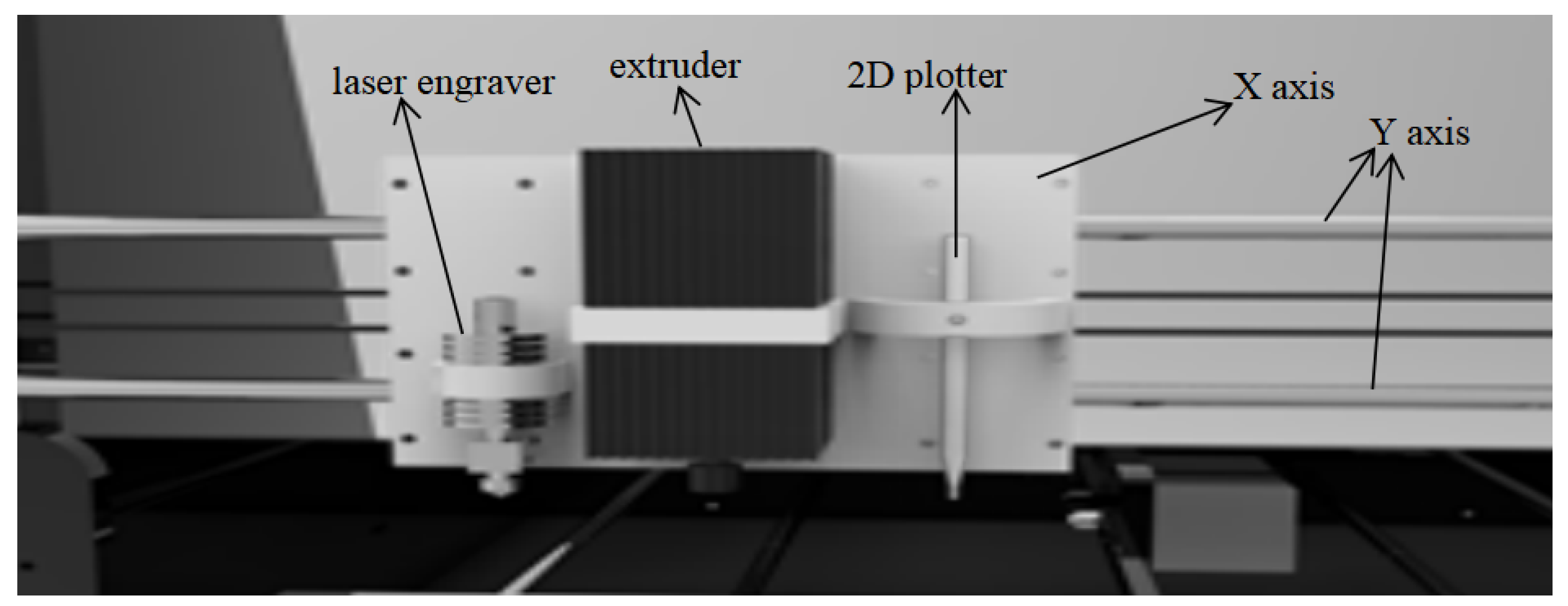
3.1. Laser Engraving Machine Working Principle

The engraving machine studied in this article is a modification of a 3D printer designed in previous literature [20], as shown in Figure 1.

The engraving machine consists of a laser engraver, extruder, 2D plotter, control circuit, controller, and stepping motor. The laser engraving machine has two axes; each is driven by a stepping motor, and the movement of motor on the X axis and Y axis are independent. First, the computer that connects to the laser engraving machine needs to extract the pixels of the image and store the pixels in a matrix. Second, the computer converts the pixels’ matrix into G-code. Finally, the G-code is downloaded to the controller, which controls the laser engraver to draw the image in a 2D plane.

Assume there is an engraving point (r) on the platform shown in Figure 1. The laser engraver needs to move from r to the coordinate position where the next engraving point (p) is located. At this time, the laser engraver has three movement routes. As shown in Figure 2, the first is where the laser engraver moves from r to p through n, the second is where the laser engraver moves from r to p directly, and the third is where the laser engraver moves from r to p through m.

Among the above three movement routes, the first and second movement routes need to use pulse width modulation (PWM) to precisely control the speed of the stepping motors of the x and y axes. The first route requires the motors of both axes to rotate simultaneously, and the speed ratio of both axis is satisfied $\gamma =\frac{n_y}{n_x}=tan\alpha$. The second route requires the motors of both axes to rotate at the same speed, and the speed ratio is satisfied $\gamma =\frac{n_y}{n_z}=tan\beta$, where $\beta$ is 45. $n_y$ represents the speed of the Y-axis motor, and $n_x$ represents the speed of the X-axis motor. When the laser engraver moves from point r to point n, the motor of the axis stops, and the motor of the X axis continues to move and drive the laser engraver from point n to point p. The third route needs to make the motor of the X(Y) axis rotate; when the laser engraver moves to the X(Y) axis coordinate position of the engraving point p, the motor of the X(Y) axis stops and the motor of the Y(X) axis rotates. When the laser engraver moves to the X(Y) axis coordinate position of the engraving point p, the motor of the X(Y) axis stops.

In the following, we analyze the time costs of three movement routes, where we do not consider the conduction time of switching devices, such as thyristors. Assume that the speed of the motor is a linear change related to the movement speed of the X/Y axis, where the proportional value between the speed of the two motors is equal to the proportional value between the movement speed of the X axis and Y axis. Let A denote the movement speed on the X axis, B denote the movement speed on the Y axis, $(x_1,y_1)$ denote the coordinate position of the engraving point r, $(x_2,y_2)$ denote the coordinate position of the engraving point p, and $t_1,t_2,t_3$ denote the movement time using the first, second, and third movement methods, respectively. $t_1,t_2,t_3$ can be computed as follows:

$$t_1=\frac{|x_1-x_2|}{A}=\frac{|y_1-y_2|}{B}$$

(1)

$$t_2=max\{\frac{|x_1-x_2|}{A},\frac{|y_1-y_2|}{B}\}$$

(2)

$$t_3=\frac{|x_1-x_2|}{A}+\frac{|y_1-y_2|}{B}$$

(3)

For the second movement route, if $\left|x_1-x_2\right|>|y_1-y_2|$, the motor of the X axis rotates at A speed, and the motor of the Y axis rotates at B speed, which is equal to A. Obviously, we should take the maximum run time of the motor of the X axis and the motor of the Y axis. The run time of the X-axis motor is $\frac{|x_1-x_2|}{A}$, which is the same as for the first route. Similarly, if $\left|y_1-y_2\right|>|x_1-x_2|$, the time of the second route and the first route is also equal. Equations (1)–(3) show that the time costs of the first and second movement routes are equal and are less than the third movement route. However, the first movement route has two disadvantages. One is that the route has a high requirement for control accuracy, because this route requires adjusting the duty cycle using PWM to change the speed ratio of the two stepping motors. The other is that if using the first route, the computer program is more suitable for large-scale image engraving tasks. In addition, because the third route takes more time, we choose the second route as the engraver’s movement method, where the engraving distance is defined as the infinite norm, $\left|\right|$r−p${\left|\right|}_{\infty }$, of the engraving points r and p.

For the engraving methods, there are three traditional methods of engraving. The first method is that the engraver works line by line along a direction, which can be the X-axis positive or negative direction or the Y-axis positive or negative direction. For example, the engraving machine works line by line along the X-axis positive direction and Y-axis positive direction. The second method is that the engraver first engraves a line along a direction; then, it engraves the next line along the opposite direction. For example, the engraver engraves a line along the X-axis and Y-axis positive direction; then, it engraves the next line along the X-axis negative direction and Y-axis position direction. Both methods are known as the dot engraving method. The third method is the greedy method, which starts with the edge point of the image, follows with the closest point of the previous point from all the unengraved points, and finishes the whole engraving [9].

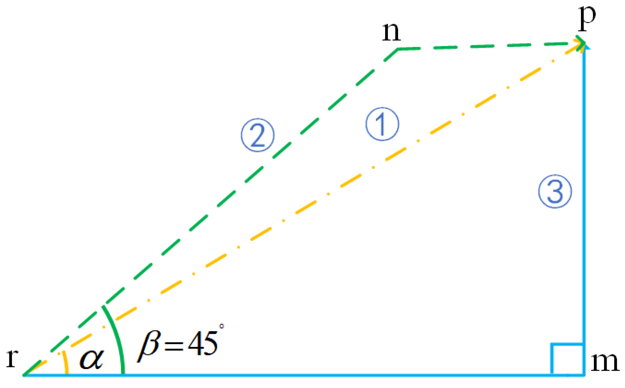
3.2. Mathematical Model

For the image engraving, there are three tasks that need to be finished in advance. One is that the image needs to be converted into a binary image using the Floyd-Steinberg dithering method, which can convert an image of any size into pixels of any size. The larger the pixel size of the same image after conversion, the closer the binary image is to the original image. The next one extracts the coordinates of black pixels in the binary image according to a certain sequence. The last one constructs a set of laser engraving points and stores them in a list in turn. Let C represent the set of laser engraving points, denoted as $C=\{c_1,c_2,\cdots ,c_N\}$. Let $d_{ij}$ denote the infinite number from the laser engraving point $c_i$ to the laser engraving point $c_j$, where $i,j\in N$. Let the binary variable $r_{ij}$ denote whether there is an existing a route between two laser engraving points ($c_i$ and $c_j$). If there is a route, $r_{ij}=1$; otherwise, $r_{ij}=0$. The mathematical model of minimizing the trajectory of the engraving machine can be expressed as the following optimization problem [21]:

$$min\sum _{i=1}^n\sum _{j=1}^n{d}_{ij}{r}_{ij}$$

(4)

The constraints are shown in Equations (5)–(7).

$$\sum _{j=1}^N{r}_{ij}=1,i=1,2,\cdots ,N,j\cap i=\varphi$$

(5)

$$\sum _{i=1}^N{r}_{ij}=1,j=1,2,\cdots ,N,i\cap j=\varphi$$

(6)

$$r_{ij}=\left\{0,1\right\},i,j\in N$$

(7)

4. Multifactorial Evolutionary Algorithm

In this section, we discuss the main idea of the multifactorial evolutionary algorithm (MFEA), its implementaion scheme, and its advantage in solving the large-scale TSP.

Solving problems in reality is not always isolated, as the experience of solving historical issues is helpful to solve similar new problems. For example, people who can ride bikes easily learn to drive motorcycles [22,23,24,25]. Because we use the clustering algorithm to divide the city group into some medium-scale city groups, and then use the clustering algorithm to divide each medium-scale city group into some small-scale city groups, the small-scale city groups contained in each medium-scale city group have certain similarities in spatial distribution. Considering the internal similarity between the optimized small-scale TSP, the knowledge obtained by EAs in solving a small-scale TSP may be transferred to EAs solving other small-scale TSPs to enhance EAs’ search ability. Therefore, MFEA is used to solve the small-scale TSP so as to realize knowledge exchange between EAs solving different small-scale TSPs.

MFEA is a specific implementation of multifactorial optimization (MFO) based on the GA [26,27], which was first proposed in literature [28]. The specifications include three steps.

First, MFEA generates an initial population of N individuals. Each individual is encoded into a unified space and can be translated into a task-specific solution with respect to any of the optimization tasks. For each individual in all tasks, MFEA defines four indicators: the factorial cost, factor ranking, scalar fitness, and skill factors. The four indicators are defined below:

1.

Factorial Cost: If the $i\left(i=1,2\cdots N\right)$ individual $p_i$ in populations was evaluated on the j task $T_j$, the $p_i$’s factorial cost ${\phi }_{ij}$ is equal to the fitness value of $p_i$ on $T_j$, i.e., ${\phi }_{ij}$ is calculated according to the object function $T_j$ and $p_i$. Assume there are M tasks; each individual’s factorial cost is a M-dimensional row vector and each dimension represents the fitness value of the individual in this task.

2.

Factorial Rank: If the individual $p_i$ is evaluated on the $jth$ task $T_j$, $p_i$’s factorial rank is equal to the position of $p_i$ according to an ascending sequence of factorial cost among all the individuals that calculated factorial cost on task $T_j$. If there are two or more individuals that have equal factorial cost in one task, their factorial rank will be determined randomly. Factorial rank reflects the quality of individuals in the task. If the individual’s factorial rank is smaller in the task, the performance of the individual is better in this task.

3.

Scalar Fitness: The individual $p_i$’s scalar fitness $f_i$ is defined as the reciprocal value of the best factorial rank in the task M, i.e., $f_i=\frac{1}{r_{ij}},r_{ij}\in min(r_{i1},r_{i2},\cdots ,r_{iM})$. The bigger the individual’s scalar fitness, the better the individual is.

4.

Skill Factor: The skill factor $s_i$ of the individual $p_i$ is the number of tasks that has the smallest factorial rank in all tasks, i.e., $s_i=argmin(r_{i1},r_{i2},\cdots ,r_{iM})$. If the individual $p_i$’s skill factor is equal to 1, $p_i$ will evaluate Task 1.

Second, a child population is generated by executing the selection mating operation on the current population. Each child inherits the corresponding skill factor through vertical cultural propagation operation; that is, each child belongs to a certain task and is evaluated on this task.

Third, the scalar fitness of all individuals of the parent population and the child population is updated, and N individuals that have the optimum scalar fitness are selected to make up the next population.

The above steps are implemented until the termination condition is met. The MFEA algorithm framework is described as follows:

MFEA Algorithm Framework

Input: Initialize a population which has N individuals as the parent population

Output: Solution of each task

1. Evaluate all individuals in the population on per task, calculate each individual’s factorial cost,

factorial rank, scalar fitness, and skill factor

2. While not satisfying termination conditions

3.       The child population is generated by executing the selection mating operation on the parent

population

4.       Execute vertical cultural propagation operation on child population to determine which

task will be evaluated by the child population individual

5.       Update the scalar fitness of the parent population and the child population

6.       Select N individuals which have the bigger scalar fitness in the parent population and the

child population to form the next generation population

7. End while

Knowledge transfer between different tasks mainly occurs in selection mating and vertical cultural propagation. The algorithm frameworks for selection mating and vertical cultural propagation are shown below.

Selection Mating

Input: Randomly select two individuals $p_i$ and $p_j$ in the parent population, random mating

probability $rmp\in \left[0,1\right]$

Output: Two child individuals $c_i$ and $c_j$

1. Generate a random number $rand$ between $[0,1]$

2. If ($p_i$ and $p_j$ have same skill factor) or ($rand<rmp$)

3.       Use cross operator for $p_i$ and $p_j$ to generate two child individuals $c_i$ and $c_j$

4. Else

5.       Use variation operator for $p_i$ and $p_j$ to generate two child individuals $c_i$ and $c_j$

6. End

Vertical Cultural Propagation

Input: Child individual $c_i$ without skill factor

Output: Child individual $c_i$ that has skill factor

1. If ($c_i$ is generated by two parent individuals $p_i$ and $p_j$ through cross operation)

2.       Generate a random number $rand$ between $\left[0,1\right]$

3.       If ($rand<0.5$)

4.             $c_i$ obtains $p_i$ skill factor

5.       Else

6.             $c_i$ obtains $p_j$ skill factor

7.       End

8. Else

9.       If ($c_i$ is generated by $p_i$ through variation operation)

10.             $c_i$ obtains $p_i$ skill factor

11.       Else

12.             $c_i$ obtains $p_j$ skill factor

13.       End

14. End

5. Three-Layered and Parallel Multifactorial Evolutionary Algorithm

In this section, we propose an optimal algorithm based on MFEA using three-layered clustering and multi-process parallel optimization, called 3L-MFEA-MP, which aims to minimize the trajectory in the image engraving according to the mathematical model in Section 3.

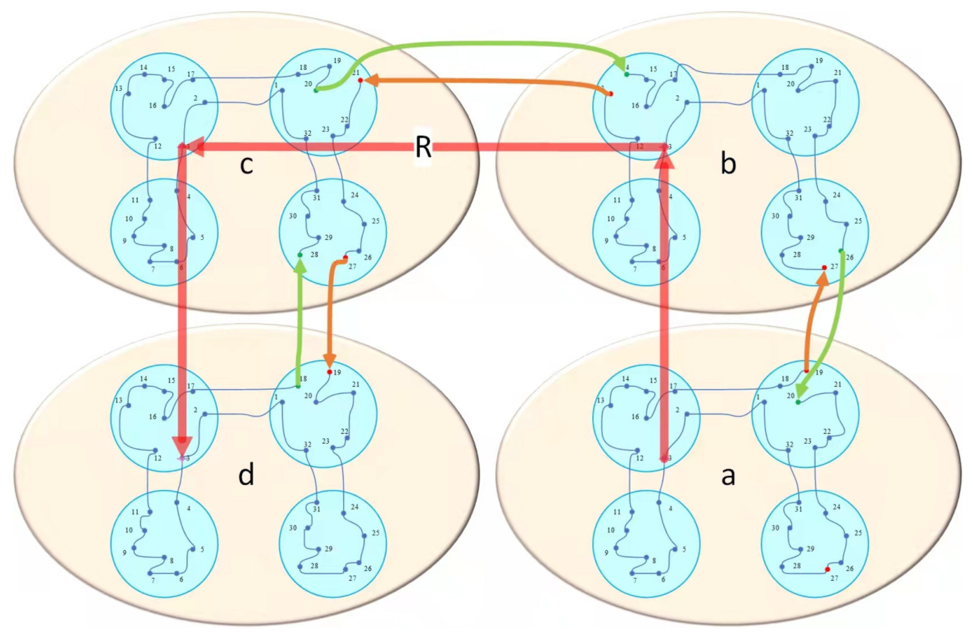
5.1. Three-Layered Evolution Optimization Framework

Considering that the image to be engraved usually contains tens of thousands or more pixels, how to reduce the computational cost and time of the path optimization is a crucial issue. We propose a three-layered evolution optimization framework motivated by the methods presented in previous studies [15,16,19], which uses clustering algorithms to transform a large-scale city group into various medium-scale and small-scale city groups. The three-layered structure and city group connection diagram is shown in Figure 3.

In Figure 3, the ellipses A, B, C, and D represent the four medium-scale city groups, respectively, which are divided into large-scale city groups by the K-Medoids algorithm. The four circles in each ellipse represent the four small-scale city groups, which are divided into medium-scale city groups by the K-Medoids algorithm. The thick red arrows in the figure represent the connection sequence between medium-scale city groups, whereas the orange and green thin arrows represent the connection sequence and connection method of small-scale city groups contained in different medium-scale city groups. The blue thin lines represent the connections between small-scale city groups within each medium-scale city group.

Assume $K_1,K_2,\cdots ,K_N$ denote the centers of medium-scale city groups in the top layer and $M_1,M_2,\cdots ,M_N$ denote each medium-scale city group. Assume $K{K}_1,K{K}_2,\cdots ,K{K}_L$ denote the centers of small-scale city groups in the middle layer and $S_1,S_2,\cdots ,S_L$ denote each small-scale city group. Therefore, the bottom layer consists of $N*L$ small-scale city groups. In the top layer, we use the GA to optimize the TSP that is composed of the center of each medium-scale city group so as to obtain a non-closed path R, $R=\left\{R_i=Index\left(K_j\right)|i,j=1,2,\cdots ,N\right\}$. Here, $Index\left(K_j\right)$ represents the serial number of city j, $R_1$ stores the serial number of the starting city, $R_N$ stores the serial number of the ending city, and $R_1$ and $R_N$ are not connected. In the middle layer, we use the GA to optimize the TSP that is composed of the center of each small-scale city group in each medium-scale city group to obtain N non-closed paths $r^j,j=1,2,\cdots ,N$, $r^j=\left\{r_i=Index\left(K{K}_m\right)|i,m=1,2,\cdots ,L\right\}$. Here, $Index\left(K{K}_m\right)$ represents the serial number of city m, $r_1$ stores the serial number of the starting city, $r_L$ stores the serial number of the ending city, and $r_1$ and $r_L$ are not connected. In the bottom layer, we use MFEA to optimize each small-scale city group TSP to obtain $N*L$ closed paths $P^j,j=1,2,\cdots ,N*L$, $P^j=\left\{P_i=Index\left(C_s\right)|i=1,2,\cdots ,Q+1,s=1,2,\cdots ,Q\right\}$, where $Index\left(C_s\right)$ represents the serial number of city s, $P_1$ stores the serial number of the starting city, $P_Q$ stores the serial number of the ending city, $P_1$ and $P_Q$ are connected, and $P_{Q+1}$ stores the serial number of the starting city.

Then, we use the optimization result of the middle layer to connect small-scale city groups in each medium-scale city group into a whole. Finally, the optimization result of the top layer is used to connect the medium-scale city groups into a whole. The three-layered evolution optimization framework is shown in Algorithm 1, and the flow chart of the city groups’ connection method is shown in Figure 4.

Algorithm 1 Three-Layered Evolutionary Optimization Framework.

Input: City coordinate and city serial number $\left(C=\left\{C_i=(x_i,y_i)|i=1,2,\cdots ,W\right\}\right)$, number of clusterings N (even) and iterative number $K_{max}$ of upper layer’s K-medoids, number of clusterings L (even) and iterative number $K{K}_{max}$ of middle layer’s K-medoids, population size and maximum number of iterations $iter\_max1$ of upper layer’s GA, population size and maximum number of iterations $iter\_max2$ of middle layer’s GA, population size and maximum number $iter\_max3$ of iterations of MFEA

Output: Optimal path and optimal path length

1. Use K-medoids divide W citys into N medium-scale city groups, the centers of medium-scale city groups are $\left\{K_i\right|i=1,2,\cdots ,N\}$

2. Use K-medoids divide each medium-scale city groups into L small-scale city groups, the centers of small-scale city groups are $K{K}_i^j|i=1,2,\cdots ,N,j=1,2,\cdots ,N*L\}$

3. Use GA to optimize the TSP that is composed of the centers of N medium-scale city groups to obtain optimal path R

4. Use GA to optimize the TSP that is composed of the center of L small-scale city groups within each medium-scale city group to obtain N city groups’ optimal path $r^j,j=1,2,\cdots ,N$

5. Randomly divide small-scale L city groups within each medium-scale city group into $L/2$ city combinations to obtain a total of $N*L/2$ city combinations $O_m^i$ $\left(O_m^i=\left\{O_m^i=(L_j^i,L_k^i)|i=1,2,\cdots ,N,m=1,2,\cdots ,L/2,j,k\in \{1,2,\cdots ,L\},j\cap k=\varnothing \right\}\right)$

6. Use $MFEA$ to optimize $N*L/2$ city combinations, respectively, to obtain $N*L$ city groups’ optimal path $P_j,j=1,2,\cdots ,N*L$ and optimal path length $Lengt{h}_j$

7. According to the best path $r^j$ to connect L small-scale city groups within each medium-scale city group to a whole

8. According to the best path R to connect N medium-scale city groups to a whole

5.2. Parallel Optimization of the Path in the Bottom Layer

Modern computers typically have multiple processor cores. However, adopting the multiple processor core to implement computational tasks for computationally intensive jobs can significantly reduce the computation time and increase the calculation complexity of the algorithm. Most existing research has applied Python or Matlab as a programming language to solve the large-scale TSP, although MATLAB’s parallel processing toolkit is only suitable for simple loop and numerical calculations. Moreover, the code based on Python usually uses the CPython compiler, whose main feature is that it can only be calculated by using the CPU single core. Because of the existence of GIL in CPython, we cannot make full use of the CPU’s multi-core computing performance. Therefore, we redesigned the algorithm to solve the path optimization problem in the bottom layer so that the algorithm has the ability to calculate multiple small-scale TSPs in a parallel scheme.

Modern CPUs usually apply hyper-threading technology; that is, one entity CPU can provide two logical threads. Therefore, we define the size of the process pool N as the following formula:

$$N<2\ast CP{U}_{-}num-1$$

(8)

Frequent switches of the process incur additional costs, so we give calculation-intensive processes higher priority. These processes can compete with the computer processor in other processes, so we need to reserve some process space for other processes. For the CPU with a C core and 2C threads, we designed the size N of the process pool according to Equation (9), where H represents the number of logical processors reserved for other processes.

$$N<2\ast C-h$$

(9)

The bottom-path parallel optimization algorithm frame is shown in Algorithm 2.

Algorithm 2 Parallel Path Optimization in the bottom layer.

1. Create N processes from the CPU process pool, N less than $2C-1$, C is the number of CPU

cores

2. N processes sequentially select tasknum city groups according to the optimal path $r^j$ of middle

layer, tasknum is the number of tasks that can be optimized by MFEA

3. We use MFEA to optimize city groups that had been selected by each process

4. While (The process i has completed the current optimization task and there are city groups that

are not selected by other processes)

5.       The process i select sequentially select tasknum city groups that are not selected by other

processes according to the optimal path $r^j$

6.       We use MFEA to optimize city groups that had been selected by process i

7. End While

6. Simulation Experiment and Performance Analysis

In this section, we describe some simulation experiments performed to evaluate our algorithm. We first describe the simulation environment and then compare the performance of our algorithm on four classical datasets using four algorithms, including our proposed algorithm.

6.1. Experimental Setup

To evaluate the performance of the proposed algorithm, 3L-MFEA-MP, we carried out a series of simulation experiments. All experiments were performed on the ShanHe Super Computer App Center, with a 24-core Intel Xeon CPU and 96-GB RAM and the Cascade Lake CPU software architecture. Our experiments were performed on four large-scale TSP datasets, namely mona-lisa 100K, vangogh 120K, venus 140K, and earring 200K. To reduce the irregularity of the experimental results, each experiment was implemented five times with the same parameters.

In this study, we carried out three comparison experiments, including a comparison of the proposed algorithm with other intelligent algorithms with classical methods to investigate the run time and solution quality of the proposed algorithm. In addition, we implemented experiments on a personal computer, with different engraving movement routes and in real engraving machines to evaluate the performance of our algorithm.

6.2. Comparison and Analysis with Other Algorithms

In this section, we describe three other algorithms developed, including the parallel optimization two-layered multi-factorial evolutionary algorithm (2L-MFEA-MP), the three-layered multi-factorial evolutionary algorithm (3L-MFEA), and the parallel optimization three-layered genetic algorithm (3L-GA-MP).

We developed 2L-MFEA-MP to evaluate the superiority of the three-layered evolutionary optimization framework proposed in Section 5.1 by comparing 3L-MFEA-MP with 2L-MFEA-MP. Here, 2L-MFEA-MP uses the two-layered evolutionary optimization framework proposed in literature [8]. The top layer uses the GA algorithm, whereas the bottom layer uses the MFEA algorithm, which uses the parallel optimization scheme proposed in Section 5.2. We developed 3L-MFEA to investigate the superiority of the parallel optimization scheme proposed in Section 5.2 by comparing 3L-MFEA-MP with 3L-MFEA. Here, 3L-MFEA adopts the three-layered evolutionary optimization framework proposed in Section 5.1, the upper and middle layers use GA, and the bottom layer uses MFEA. We developed 3L-MFEA to verify the superiority of migration optimization between the different tasks proposed in Section 5.1. Here, the 3L-GA-MP uses the three-layered evolutionary optimization framework proposed in Section 5.1. The upper, middle, and bottom layers all use the GA, and the bottom layer uses the parallel optimization scheme proposed in Section 5.2.

The main parameter settings of the experiments are shown in

Table 1. The main parameters of the experiment.

Algorithm	Pop_Size	Max_Iteration	Mating	Mutation	Vertical Cultural	Number of
			Rate	Rate	Propagation Rate	Process Pool
3L-GA-MP	100	500	0.7	0.03	NaN	40
2L-MFEA-MP	100	500	0.7	0.03	0.7	40
3L-MFEA-MP	100	500	0.7	0.03	0.7	40
3L-MFEA	100	500	0.7	0.03	0.7	1

. pop_size is the population size, and max_iteration is the maximum number of iterations. For the MFEA, we adopted the method of knowledge transfer between two subtasks, so the sum of the population size of the two subtasks was 100, and the population size allocated to each subtask was less than 100. Note that to ensure a fair comparison, we did not use the GA library optimized by other scholars for the GA but rather the GA written by us. MFEA and GA used the same crossover operator and mutation operator.

First, we investigated the run time and the path length of four algorithms.

Table 2. Simulation results of three algorithms on four large-scale TSP data sets.

Test Case	Test Algorithm	Optimal Value	Average Value	Average Time (s)
mona-lisa 100K	3L-GA-MP	6,573,858.48	6,580,451.45	1169.22
	2L-MFEA-MP	7,320,781.49	7,338,432.16	1257.24
	3L-MFEA-MP	6,513,685.57	6,525,173.32	1030.72
vangogh 120K	3L-GA-MP	7,484,062.34	7,492,754.71	1433.82
	2L-MFEA-MP	10,355,545.62	10,368,895.74	1312.9
	3L-MFEA-MP	7,423,925.39	7,430,062.76	1256.78
venus 140K	3L-GA-MP	7,778,041.94	7,786,448.81	1734.2
	2L-MFEA-MP	10,757,158.96	10,782,308.25	1666.52
	3L-MFEA-MP	7,718,440.84	7,724,200.98	1518.13
earring 200K	3L-GA-MP	9,433,863.79	9,438,150.22	2658.72
	2L-MFEA-MP	13,419,519.17	13,438,280.99	2639.42
	3L-MFEA-MP	9,365,519.37	9368743.37	2382.31

shows the results, including the optimal value, average value, and average time obtained by four algorithms from five experiments. Here, the optimal value represents the shortest path length, the average value represents the average of the path length, and the average time represents the average of the run time obtained from five simulation experiments.

From Table 2, we infer the following. First, the path length of the solution for 3L-MFEA-MP was 0.8% smaller than that of 3L-GA-MP. The run time of the solution for 3L-MFEA-MP was 12% smaller than that of 3L-GA-MP. This is because using knowledge transfer between the subtasks of the bottom layer in MFEA can improve the convergence speed and avoid the fall into the local optimum; this is so that 3L-MFEA-MP can reduce the computation time and obtain a shorter path.

In addition, 3L-MFEA-MP had two advantages compared with 2L-MEFA-MP. One is that the calculation speed of 3L-MFEA-MP was improved slightly. For example, the computation time on mona-lisa 100K was reduced by about 22%. The other is that the path length of 3L-MFEA-MP was greatly shortened; for example, the path length solved on vangogh 120K, venus 140K, and earring 200K was reduced by 28%, 28%, and 30%, respectively. This is because the size of the city groups obtained by clustering twice was smaller than the size obtained by clustering only once, which helped reduce the computational complexity of MFEA on each city group. This shows that the three-layered evolutionary optimization framework has great advantages compared with the two-layered evolutionary optimization framework proposed in the literature [15,16,19].

Second, we investigated the advantage of the multi-process compared with the single-process algorithm.

Table 3. Simulation results of multi-process algorithm and single process algorithm on four large-scale TSP data sets.

Test Case	Test Algorithm	Optimal Value	Average Value	Average Time (s)
mona-lisa 100K	3L- MFEA	6,523,192.43	6,528,841.22	6317.92
	3L-MFEA-MP	6,513,685.57	6,525,173.32	1030.72
vangogh 120K	3L- MFEA	7,422,190.16	7,425,983.21	4645.26
	3L-MFEA-MP	7,423,925.39	7,430,062.76	1256.78
venus 140K	3L- MFEA	7,716,474.45	7,721,780.09	8933.52
	3L-MFEA-MP	7,718,440.84	7,724,200.98	1518.13
earring 200K	3L- MFEA	9,362,148.68	9,367,856.14	13,069.06
	3L-MFEA-MP	9,365,519.37	9,368,743.37	2382.31

shows the results, including the optimal value, average value, and average time. Here, the optimal value, average value, and average time definitions are as described in Table 2.

From Table 3, we can observe that the path length obtained by 3L-MFEA-MP was almost the same as 3L-MFEA; their difference was only about 0.05%. However, the computation time obtained by 3L-MFEA-MP was only about one fifth that of 3L-MFEA. This is because multiple process pools can optimize multiple subtasks at the same time, whereas a single process pool can only optimize one subtask once, which demonstrates the effectiveness of the proposed subtask parallel optimization method.

6.3. Comparison and Analysis with the Previous Classical Methods

In this experiment, we compared our algorithm with the well-known parallel GA proposed in [18] and the dot matrix engraving method (DM) introduced in [29].

Table 4. Comparison of the three algorithms.

Test Case	Parallel  GA	DM	3L-MFEA-MP
mona-lisa 100K	5,757,191	282,061,784.2	6,525,173.32
vangogh 120K	6,543,609	328,731,852.6	7,430,062.76
venus 140K	6,810,665	315,655,207.1	7,724,200.98
earring 200K	7,619,953	353,401,270.8	9,368,743.37

shows the results, which are described as the average of the path lengths obtained from five experiments. Table 4 illustrates that 3L-MFEA-MP was much smaller than the DM method in terms of the path length, and the path length obtained by 3L-MFEA-MP was only about $1/40$ of the path length obtained by DM. However, the path length obtained by 3L-MFEA-MP was longer than parallel GA, and the path length obtained by 3L-MFEA-MP was about 13% longer than parallel GA. Because our aim was to find the shortest engraving path in an acceptable time, it would be acceptable even if 3L-MFEA-MP was longer in path length compared to parallel GA.

6.4. Experimental Results Running on a Personal Office Computer

The performance of the computer affects the run time of the algorithm, and the number of processes determines the number of tasks for parallel optimization, which indirectly determines the run time of the algorithm. Considering that the super computer does not have wide application prospects in the engraving industry at present, to evaluate the industrial value of 3L-MFEA-MP, we performed various experiments using 3L-MFEA-MP on a personal office computer. The computer parameters were AMD Ryzen 7 5800H with 3.2 GHz, 8 cores, and 16 threads CPU with 16-GB RAM. The algorithm parameter settings were the same as in Section 6.2, and the number of process pools was set to 10.

Table 5. Running time of the algorithm on two configurations of computers.

Test Case	Super Computer (s)	Ordinary Computer (s)	Relative Difference (E)
mona-lisa 100K	1030.72	1129.49	8.74%
vangogh 120K	1256.78	1373.16	8.48%
venus 140K	1518.13	1572.5	3.46%
earring 200K	2382.31	2204.85	8.05%

shows the results, which are described as the average optimization time running our algorithm five times on a super computer and personal office computer. Assume E denotes the relative difference between two different computers, and E can be expressed as in Equation (10).

$$E=\frac{|Re{s}_c-Re{s}_p|}{Re{s}_p}\times 100\%$$

(10)

where $Re{s}_c$ represents the result of the super computer, and $Re{s}_p$ is the result of the ordinary computer.

Based on the analysis shown in Table 2 and Table 5, we can observe that the run time on an office computer was about 8% longer than that on the super computer. However, the results on the personal office computer are still in an acceptable range because the configuration of the supercomputer was far better than that of the personal office computer, and the number of processes was set to 40 on the supercomputer, which is four times higher than that set on the personal office computer.

However, in Table 5, note that a shorter time was achieved on a conventional computer when calculating the last and largest earring pattern as compared to a supercomputer, which is counterintuitive. This is because our algorithm first needs to cluster the city points of the TSP dataset and then use EAs for path optimization. For example, to cluster the mona-lisa 100K dataset containing 100K city points, the location information of all city points must be loaded into memory. Each city point’s location information contains two float64 variables, which is 8 B. The storage matrix corresponding to 100K city points is about 74.5 GB. The supercomputer has 96G RAM and can cluster all city points at once, as shown in Figure 5a. However, the conventional computer with 16 GB of RAM has to split city points set into different areas in row(column) priority, cluster them separately, and then regroup them, as shown in Figure 5b. As the time complexity of the clustering algorithm we used is not linear, the time cost of clustering large-scale city points at one time was greater than that of splitting large-scale city points into multiple small-scale city points. However, by comparing Figure 5a,b, it is easy to conclude that clustering all city points at one time had a higher accuracy than splitting and clustering the data first. Therefore, with the increase in the scale of the dataset, the supercomputer spent more optimization time when obtaining a higher-precision optimization path than the conventional computer. In addition, note that in order to control variables, we stipulated that the number of clustering points after merging should be the same, and the number of splitting clustering should be rounded down by using the maximum RAM of the computer as the standard.

6.5. Experimental Results Based on the Movement Route of the Engraving Machine

Furthermore, all of the above experiments were performed based on the L2 norm, which defines the distance between two city points, $c_i$ and $c_j$. According to the analysis of the movement routes of the engraving machine in Section 3.1, it is clear that the distance calculated by infinite norm would obtain a shorter engraving path. Therefore, we implemented experiments using the infinite norm to evaluate the performance of our algorithm. The parameters of 3L-MFEA-MP were set to be the same as those in Section 6.2.

Table 6. Results of algorithm runs with infinite norm.

Test Case	Average Path Length	Average Time (s)	Relative Difference
mona-lisa 100K	5,817,834	821.99	16.60%
vangogh 120K	6,633,908	992.831	16.80%
venus 140K	6,880,842	1162	13.10%
earring 200K	8,342,285	1648.42	13.40%

tabulates the results, including the average path length, average time obtained by 3L-MFEA-MP, and relative difference. Here, the relative difference indicates the relative difference between the path lengths obtained by 3L-MFEA-MP based on the L2 norm and the path lengths obtained by 3L-MFEA-MP based on the infinite norm.

6.6. Experimental Results of Real Engraving Machine

Furthermore, to evaluate the effectiveness of 3L-MFEA-MP, we engraved the path obtained by 3L-MFEA-MP and DM on a real engraving machine. First, we converted the paths obtained from 3L-MFEA-MP in Section 6.2 and the paths obtained from the DM engraving method in Section 6.3 into G-codes. Then, we input these paths into the engraving machine and started it up.

Table 7. Real engraving machine operation results.

Test Case	3L-MFEA-MP	DM	Relative Difference
mona-lisa 100K	2141	24,904	1063.19%
vangogh 120K	2275	31,116	1267.73%
venus 140K	2447	29,861	1120.31%
earring 200K	3180	35,931	715.44%

shows the engraving machine running time(s) and relative difference, where the relative difference represents the engraving time’s relative difference between the two algorithms.

In addition, to compare the difference in performance of the real engraving machine between the engraving paths obtained by 3L-MFEA-MP and DM, we used a 2D image plotter to plot the engraving path of monalisa 100K obtained by 3L-MFEA-MP, as shown in Figure 6.

Note that Figure 6 shows two longer linear “scratches” and a black spot on Mona Lisa’s neck, because we used a waterborne pen parallel to the laser engraving head to visualize the route. The linear “scratches” represent the movement path of the laser engraving machine, and the laser only works at the endpoint. In addition, our engraving machine needs to calculate some parameters and wait seconds before engraving so that the static waterborne pen prints black spots, which is not an algorithm error.

7. Conclusions

In this article, to address the trajectory minimization problem in large-scale image engraving, we propose a three-layered multifactorial evolutionary algorithm with parallelization. Under the proposed scheme, we made three contributions. The first is clustering the large-scale city group to the medium-scale and small-scale city group, the second is the development of efficient knowledge transfer mechanisms between subtasks, and the third is the design of parallel optimization based on multi-process. In simulation experiments, empirical studies on four large-scale datasets have been conducted to assess the performance of the proposed 3L-MFEA-MP. The results demonstrate that 3L-MFEA-MP has greater advantages compared with the currently popular two-layered evolutionary optimization algorithm in terms of running time and path length. Comparing 3L-MFEA-MP with the traditional DM engraving method, the engraving path length obtained by 3L-MFEA-MP is only $1/40$ of that obtained by the DM method.

In future research, we will improve the method of migration learning for the subtask in the bottom layer to reduce the impact from negative migration.

References

1. Fraser, A.; Deschênes, J.M. True Traceability Enabled by In-Line Laser Marking of Lead and Zinc Ingots. In Proceedings of the PbZn 2020: 9th International Symposium on Lead and Zinc Processing, San Diego, CA, USA, 23–27 February 2020; Springer: Cham, Switzerland, 2020; pp. 767–775. [Google Scholar]
2. Sundaria, R.; Nair, D.G.; Lehikoinen, A.; Arkkio, A.; Belahcen, A. Effect of laser cutting on core losses in electrical machines—Measurements and modeling. IEEE Trans. Ind. Electron. 2019, 67, 7354–7363. [Google Scholar] [CrossRef]
3. Gregory, G.; Punnen, A.P. (Eds.) The Traveling Salesman Problem and Its Variations; Springer Science & Business Media: Berlin, Germany, 2006. [Google Scholar]
4. Cook, W.J. In Pursuit of the Traveling Salesman: Mathematics at the Limits of Computation; Princeton University Press: Princeton, NJ, USA, 2011. [Google Scholar]
5. Ruan, L.; Zhang, L.; Wu, C. A New Tour Construction Algorism and its Application in Laser Carving Path Control. J. Image Graph. 2007, 6, 1114–1118. [Google Scholar]
6. Nini, L.; Zhangwei, C.; Shize, C. Optimization of laser cutting path based on local search and genetic algorithm. Comput. Eng. Appl. 2010, 46, 234–236. [Google Scholar]
7. Beheshti, Z.; Shamsuddin, S.M.H. A review of population-based meta-heuristic algorithms. Int. J. Adv. Soft Comput. Appl. 2013, 5, 1–35. [Google Scholar]
8. Peng, X.; Wu, Y. Large-scale cooperative co-evolution using niching-based multi-modal optimization and adaptive fast clustering. Swarm Evol. Comput. 2017, 35, 65–77. [Google Scholar] [CrossRef]
9. Durmus, E.; Mohanty, M.; Taspinar, S.; Uzun, E.; Memon, N. Image carving with missing headers and missing fragments. In Proceedings of the 2017 IEEE Workshop on Information Forensics and Security (WIFS), Rennes, France, 4–7 December 2017; pp. 1–6. [Google Scholar]
10. Jurek, M.; Wagnerová, R. Frequency Filtering of Source Images for LASER Engravers. In Proceedings of the 2019 20th International Carpathian Control Conference (ICCC), Krakow-Wieliczka, Poland, 26–29 May 2019; pp. 1–5. [Google Scholar]
11. Yang, H.; Zhao, J.; Wu, J.; Wang, T. Research on a new laser path of laser shock process. Optik 2020, 211, 163995. [Google Scholar] [CrossRef]
12. Anton, F.D.; Anton, S. Generating complex surfaces for robot milling and engraving tasks: Using images for robot task definition. In Proceedings of the 2017 21st International Conference on System Theory, Control and Computing (ICSTCC), Sinaia, Romania, 19–21 October 2017; pp. 459–464. [Google Scholar]
13. Wang, D.; Yu, Q.; Zhang, Y. Research on laser marking speed optimization by using genetic algorithm. PLoS ONE 2015, 10, e0126141. [Google Scholar] [CrossRef] [PubMed]
14. Hajad, M.; Tangwarodomnukun, V.; Jaturanonda, C.; Dumkum, C. Laser cutting path optimization using simulated annealing with an adaptive large neighborhood search. Int. J. Adv. Manuf. Technol. 2019, 103, 781–792. [Google Scholar] [CrossRef]
15. Ding, C.; Cheng, Y.; He, M. Two-level genetic algorithm for clustered traveling salesman problem with application in large-scale TSPs. Tsinghua Sci. Technol. 2007, 12, 459–465. [Google Scholar] [CrossRef]
16. Deng, W.; Xu, J.; Zhao, H. An improved ant colony optimization algorithm based on hybrid strategies for scheduling problem. IEEE Access 2019, 7, 20281–20292. [Google Scholar] [CrossRef]
17. Helsgaun, K. General k-opt submoves for the Lin–Kernighan TSP heuristic. Math. Program. Comput. 2009, 1, 119–163. [Google Scholar] [CrossRef]
18. Honda, K.; Nagata, Y.; Ono, I. A parallel genetic algorithm with edge assembly crossover for 100,000-city scale TSPs. In Proceedings of the 2013 IEEE Congress on Evolutionary Computation, Cancun, Mexico, 20–23 June 2013; pp. 1278–1285. [Google Scholar]
19. Tan, L.Z.; Tan, Y.Y.; Yun, G.X.; Zhang, C. An improved genetic algorithm based on K-medoids clustering for solving traveling salesman problem. In Proceedings of the International conference on computer science, technology and application (CSTA2016), Changsha, China, 18–20 March 2016; pp. 334–343. [Google Scholar]
20. Shahid, M.T.; Khan, M.A.; Khan, M.Z. Design and development of a computer numeric controlled 3D Printer, laser cutter and 2D plotter all in one machine. In Proceedings of the 2019 16th International Bhurban Conference on Applied Sciences and Technology (IBCAST), Islamabad, Pakistan, 8–12 January 2019; pp. 569–575. [Google Scholar]
21. Chen, J.; Wang, Y.; Xue, X.; Cheng, S.; El-Abd, M. Cooperative co-evolutionary metaheuristics for solving large-scale tsp art project. In Proceedings of the 2019 IEEE Symposium Series on Computational Intelligence (SSCI), Xiamen, China, 6–9 December 2019; pp. 2706–2713. [Google Scholar]
22. Gupta, A.; Ong, Y.S. Genetic transfer or population diversification? Deciphering the secret ingredients of evolutionary multitask optimization. In Proceedings of the 2016 IEEE Symposium Series on Computational Intelligence (SSCI), Athens, Greece, 6–9 December 2016; pp. 1–7. [Google Scholar]
23. Ong, Y.S.; Gupta, A. Evolutionary multitasking: A computer science view of cognitive multitasking. Cogn. Comput. 2016, 8, 125–142. [Google Scholar] [CrossRef]
24. Gupta, A.; Ong, Y.S.; Feng, L. Insights on transfer optimization: Because experience is the best teacher. IEEE Trans. Emerg. Top. Comput. Intell. 2017, 2, 51–64. [Google Scholar] [CrossRef]
25. Xu, Q.; Wang, N.; Wang, L.; Li, W.; Sun, Q. Multi-task optimization and multi-task evolutionary computation in the past five years: A brief review. Mathematics 2021, 9, 864. [Google Scholar] [CrossRef]
26. Tan, K.C.; Feng, L.; Jiang, M. Evolutionary transfer optimization-a new frontier in evolutionary computation research. IEEE Comput. Intell. Mag. 2021, 16, 22–33. [Google Scholar] [CrossRef]
27. Lei, Z. Design and Research of High Performance Multi-task Intelligent Optimization Algorithm Based on Knowledge Transfer; Chongqing University: Chongqing, China, 2019. [Google Scholar]
28. Gupta, A.; Ong, Y.S.; Feng, L. Multifactorial Evolution: Toward Evolutionary Multitasking. IEEE Trans. Evol. Comput. 2016, 20, 343–357. [Google Scholar] [CrossRef]
29. Anton, S.; Anton, F.D.; Constantinescu, M. Robot Engraving Services in Industry. In Service Robots; IntechOpen: London, UK, 2017. [Google Scholar]
Figure 1. Laser engraving machine converted from a 3D printer.
Electronics 11 01712 g001
Figure 2. Three types of movement for laser engraver.
Electronics 11 01712 g002
Figure 3. Three-layered structure and city group connection diagram.
Electronics 11 01712 g003
Figure 4. Three-layered structure and city groups connection diagram.
Electronics 11 01712 g004
Figure 5. Visible top layered algorithm of super computer (a) and personal computer (b).
Electronics 11 01712 g005
Figure 6. Three-layered structure and city groups’ connection diagram.
Electronics 11 01712 g006