Abstract
Permanent Magnet Synchronous Motor (PMSM) is widely used due to its advantages of high power density, high efficiency and so on. In order to ensure the reliability of a PMSM system, it is extremely vital to accurately diagnose the incipient faults. In this paper, a variety of optimization algorithms are utilized to realize the diagnosis of the faulty position and severity of the inter-turn short-circuit (ITSC) fault, which is one of the most destructive and frequent faults in PMSM. Compared with the existing research results gained by particle swarm optimization algorithms, in this paper, the methods using other optimization algorithms incorporating genetic algorithm, whale optimization algorithm and stochastic parallel gradient descent algorithm (SPGD) can acquire more stable and precise results. In particular, the method based on SPGD can obtain the most desirable performance among the methods mentioned above; that is, the relative error of short-circuit turns ratio is approximately as low as 0.03%. In addition, in the case of asymmetric input three-phase voltage and with the adverse impact of high-order harmonics at different load moments, the fault diagnosis method based on SPGD still maintains relatively satisfactory properties. Finally, the verification on the actual PMSM platform demonstrates that the SPGD can still diagnose the faulty severity.
1. Introduction
As a power device with features such as low pollution, high efficiency and strong practicality, motors have been widely used in industrial production and daily life. Among all kinds of motors, currently, PMSM possesses desired merits such as compact structure, high power and torque density and so on, which have been paid more and more attention. However, PMSM is quite prone to diverse faults in its working process because of the narrow working environment, high temperature and humidity and poor heat dissipation conditions, particularly in the emerging new energy industries involving electric vehicle and wind power generation. Common faults of PMSM include mechanical faults, permanent magnet faults and electrical faults. If these breakdowns cannot be detected and solved in a timely manner, it will lead to huge economic losses and security risks. Accordingly, the fault diagnosis of PMSM becomes more and more prevalent and significant in recent years.
A short-circuit fault is a typical electrical fault of PMSM, which specifically can be classified into inter-turn fault, inter-phase fault and phase-to-grounding fault. A short-circuit fault usually starts with an initial turn-to-turn fault. If precautionary measures are not carried out in time, it may develop into an inter-phase fault or even a phase-to-ground fault [1]. The ITSC fault in a stator is usually caused by the destruction of the insulating layer between the windings in the same phase. When this fault is neglected for a period of time, it will result in a sharp increase in local temperature and causes the whole phase to be damaged totally on account of a huge eddy current in the short circuit. Therefore, it is especially essential to detect and treat an ITSC fault. At present, there are three main ways to diagnose the ITSC fault of PMSM: the method based on analytical models, the method based on signal processing and the method based on artificial intelligence. Firstly, model-based methods generally use the states of motor or parameter estimation to diagnose, and some corresponding methods, including analyzing the difference between prediction model and actual output and introducing back electromotive force (EMF) estimation, are proposed [2,3,4]. In Ref. [2], an online inter-turn fault detection method for PMSM is proposed. This method is based on the residual analysis between the estimated current obtained from the health model and the actual current of PMSM. The residual analysis considers the back EMF estimation, inverter model and unbalanced inductance matrix. In addition, the detection method using the back EMF estimator of open-loop physics is proposed in Ref. [3]. The back EMF estimator is designed based on the current mode tracking scheme, in which the thermal and saturation aspects of the motor are considered. In Ref. [4], the main idea is to detect the instantaneous second harmonic and estimate the mechanical power based on the back EMF. The bandpass filter is used to extract the reliability index related to the severity of inter turn fault. Model-based detection methods require accurate modeling, but in practical engineering, the actual models are exceedingly difficult to represent precisely. Therefore, some fault diagnosis methods using the signal of PMSM are proposed. Among them, current and vibration signals are widely used. Vibration signals are often used in the diagnosis of bearing faults [5]. In contrast, current signal is more widely used in other faults. For the ITSC fault, Stavrou and Henao found that the fault harmonics in the stator current will increase with the stator ITSC fault [6]. In Ref. [7], the harmonic components of motor current and voltage during an ITSC fault can be analyzed by fast fourier transform (FFT) by obtaining the characteristics of the space vector spectrum. However, due to the lack of signal time information, FFT can be used only to tackle stationary signals, so wavelet analysis is also used in fault diagnosis of PMSM [8,9,10]. In Ref. [8], wavelet packet transform is used to decompose the PMSM stator current signal and calculate the signal energy value of each frequency band, which can be used as the basis of fault judgment. Although the detection methods based on signal analysis are widely used, most methods cannot predict the severity of a fault and are vulnerable to other disturbances. With the development of machine learning and artificial intelligence, many data classification and recognition methods have been proposed, such as neural network (NN), support vector machine (SVM), and fuzzy logic system (FLS). Therefore, some diagnostic methods combined with these methods have been proposed. In Ref. [11] data-driven fault diagnosis methods have also been proposed. In Ref. [12], a negative sequence analysis coupled with a fuzzy logic based approach is applied to fault detection of a PMSM. In Ref. [13], a novel fault diagnosis method using the sparse representation and support vector machine is proposed for the inter-turn short circuit fault. S. Darth et al. applied park transform and continuous wavelet transform (CWT) for signal feature extraction, and then used SVM for classification and recognition [14]. In Ref. [15], fault detection technology for detecting short-circuit fault of PMSM using artificial neural network is described and a particle swarm optimization algorithm (PSO) is used to adjust the weight of neural network. However, the knowledge-based methods depend on a mass of data leading to large calculation in the training process, so these algorithms are relatively complex.
In practical engineering, the occasions where the fault severity index of ITSC fault needed to be estimated with high diagnostic accuracy are widespread. In this paper, inspired by the above methods, a variety of heuristic algorithms are applied, firstly to diagnose the ITSC fault of PMSM, which has several advantages over the existing mainstream fault diagnosis methods. For example, compared with the traditional fault diagnosis methods based on signal processing, such as current signal analysis including Fast Fourier Transform (FFT) analysis, the proposed methods in this paper are low cost and can accurately determine the fault severity index. In addition, compared with the fault diagnosis method based on the analytic model, the proposed methods can determine the location of ITSC fault, and it is simple and easy to implement. Moreover, compared with the method based on the particle swarm optimization algorithm, which has been proposed by other scholars, it is proved that the performance of proposed methods based on heuristic optimization algorithms in this research have been improved a lot, whereas, due to the randomness of the heuristic algorithms, it is difficult to obtain satisfactory results stably. For the above shortcoming, the stochastic parallel gradient descent method has been adopted. Compared with the results acquired by heuristic algorithms, using the stochastic parallel gradient descent algorithm can achieve more stable diagnostic results with smaller relative errors.
The rest of the paper is organized as follows. The second section introduces the regular model of PMSM and the model suffered from ITSC fault of PMSM. Section 3 describes the fault diagnosis methods based on three heuristic algorithms and stochastic parallel gradient descent algorithm. A number of numerical simulations are demonstrated in Section 4. Additionally, the validation on the actual PMSM is shown in Section 5. Finally, the conclusion is drawn in Section 6.
2. Mathematical Models of PMSM
2.1. PMSM Model under Regular Operation
A typical three-phase PMSM is composed of three-phase windings and an iron core, and the armature windings are usually in wye connection. For the rotor structure, PMSM replaces the electric excitation with a permanent magnet, eliminating the field coils, slip rings and the armature. For simplicity, supposing that the three-phase PMSM is an ideal model and meets the following conditions:
- (1)
- The saturation effect of the motor core is ignored;
- (2)
- The current of the motor is a symmetrical three-phase sinusoidal current;
- (3)
- The conductivity of the permanent magnet material is zero;
- (4)
- The eddy current and hysteresis losses of the motor are excluded.
In the natural coordinates, the voltage equation and flux-linkage equation of PMSM are
where , , is three-phase winding voltage, resistance and current, respectively, and is the flux linkage of winding.
According to the electromechanical energy conversion principle, the electromagnetic torque equation of the motor can be expressed by
where p is the number of pole pairs.
In addition, the mechanical motion equation is
where , , B, is the electromagnetic torque, load torque, friction coefficient and mechanical angular velocity, respectively.
2.2. Fault Model of PMSM in ITSC
Among all the electrical faults of PMSM, the ITSC fault is the most likely fault to occur. When the PMSM is suffered from the ITSC fault, the transient impulse current may cause serious mechanical stress damage to the shaft and the end of the winding, as well as irreversible demagnetization of the permanent magnet. In order to establish a common ITSC model for PMSM without loss of generality, assume that any one- or multi-phase winding causes an ITSC fault in PMSM. The schematic and the equivalent circuit of three-phase PMSM with multi-phrase winding inter-turn short circuit (MPWITSC) are shown in Figure 1 and Figure 2. In this paper, the fault phase winding of the motor model is divided into two parts, i.e., a short-circuit part and a normal circuit part, in which the short circuit is a relatively independent current loop and forms a relatively stable magnetic field. This field will create a fourth-coupled magnetic circuit for the motor system, which destroys the stability of the original magnetic field. Then, introducing to quantify the severity of ITSC fault, and its mathematical value is the ratio of the number of short circuit turns to the total number of turns of fault phase . A phase is used to define the position where the fault occurs, and its mathematical value is the angle between the fault phase and the A-phase axis; that is 0, ±2/3. Furthermore, without loss of generality, it is assumed that the ITSC fault occurs in phase B in this paper. When the fault occurs in other phases, the analysis is the same. The kinematic Equations (5) and (6) are not only applicable to the normal working state of PMSM, but are also applicable to the PMSM suffered as a result of the ITSC fault. Thus, after derivation, and combining Equations (5) and (6), the mathematical expression of faulty model can be displayed as follows. The voltage equation is
where is the resistance of the normal part in faulty phase and is the resistance of the short-circuit part in the faulty phase. Since the demagnetization is ignored, it can be assumed that the permanent magnet flux linkage of the PMSM fault phase is composed of the normal part and the short-circuit part, which are directly proportional to . Thus, Equation (4) can be converted into
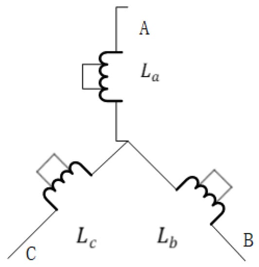
Figure 1.
The schematic of PMSM with Inter-turn fault.
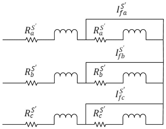
Figure 2.
The equivalent circuit of PMSM with Inter-turn fault.
The calculation of inductance parameters is necessary for the fault model of the motor. At present, there are two main methods for inductance parameter calculation. One is simple estimation calculation, which is only suitable for fault fuzzy diagnosis because of large judgment error; another method is the finite element method to calculate the inductance parameters. Although the accuracy of this method meets the requirements of fault diagnosis, the inductance parameters must be calculated repeatedly every time the simulation conditions change, so the efficiency is too low. In this paper, the proportional principle, leakage loss principle and inductance parameter consistency principle are used to calculate the inductance parameters of the motor. The calculation formula is as follows:
By substituting the inductance constant into Equations (11)–(13), the inductance matrix expression of the whole fault motor can be obtained as follows:
and the calculation process of leakage factor can be seen in reference [1].
Remark 1.
In the application of practical engineering of PMSM, due to the complex work environment and the influence of non-linear elements, many adverse phenomena will occur, such as high-order harmonics, magnetic circuit saturation and so on. It is difficult to establish a unified and simple model of PMSM. Therefore, after referring to some literature [16,17,18], we consider that the model for fault diagnosis of ITSC can be applied by the model established in the above part.
3. Fault Diagnosis for PMSM ITSC Based on Optimization Algorithms
In this section, the proposed methods based on several optimization algorithms of the fault diagnosis of ITSC for PMSMs are discussed.
3.1. The Methods Based on Heuristic Optimization Algorithms
In this paper, we apply three kinds of heuristic optimization algorithms for the diagnosis of ITSC, which contains particle swarm optimization algorithm, genetic algorithm (GA) and whale optimization algorithm (WOA).
3.1.1. Particle Swarm Optimization Algorithm
The particle optimization algorithm was proposed by J Kennedy and RC Eberhart [19], and popularized to discrete binary space by themselves [20]. It was inspired by the regularity of bird swarm activity. It is simpler than the genetic algorithm in that the particle moves towards its own optimal value and the total optimal value under randomness. Recently, this optimization algorithm has been widely applied in PMSM fault diagnosis [21] and achieved satisfactory effect. Specifically, the formulas of velocity and position of PSO are expressed as follows:
here, means the velocity of ith particle in iteration and means the position of ith particle in iteration . and are random numbers between zero and one. and represents the self-learning factor and global learning factor, respectively. In order to simulate the inertia of real objects, W is set to represent the inertia coefficient and usually cannot be zero to ensure that PSO has global search capability. The concise flow chart of this algorithm is described in Figure 3.
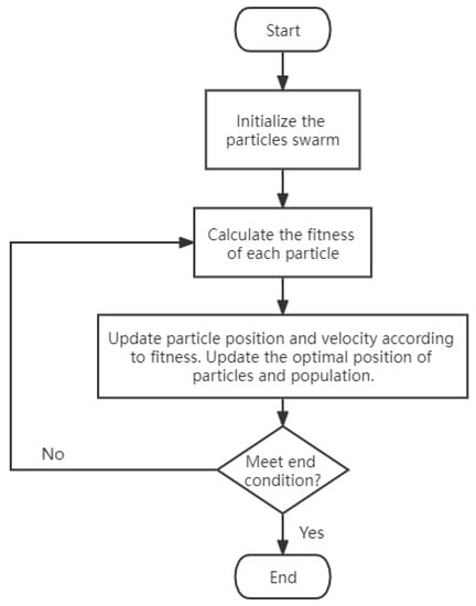
Figure 3.
The flow chart of PSO.
3.1.2. Genetic Algorithm
The genetic algorithm was inspired by Darwin’s evolution theory. Therefore, the phenomena of reproduction, hybridization and mutation in the process of natural selection and natural heredity are simulated in this algorithm. The concrete flow chart is shown in Figure 4. Since GA is more complex than other heuristic algorithms, it has a strong ability to search for optimization. When the GA is applied in the diagnosis of an ITSC fault of PMSM, the optimization objectives are the ratio of short-circuit turns and the fault phase , which are continuous and discrete, respectively. Therefore, after the selection of parents, different crossover operations should be selected for processing. For the short-circuit turns ratio, the average value of the parents will be taken as the of new individual. As for the fault phase, if the parents of the fault phase are different, one of them is randomly selected as the child of the fault phase.
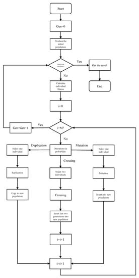
Figure 4.
The flow chart of GA.
3.1.3. Whale Optimization Algorithm
The whale optimization algorithm was first proposed in 2016 by Mirjalili et al. from Griffith University in Australia [21]. Similar to GA and PSO, it is a meta-heuristic algorithm based on group intelligence. It searches for the best solution by mimicking the predation behavior of humpback whales, which includes encircling prey and forming bubble nets. With the development of research, the algorithm has been successfully applied in wind speed prediction, feature selection, optimal reactive power scheduling, secondary allocation problem, clustering, scheduling optimization, image classification and other fields. The positions of each whale represent the solutions of the optimization questions, which are updated by these three equations as follows:
Equations (17) and (18) mean the behavior of surrounding prey. The whales will swim toward either the optimal whale or a random whale when they surround their prey. Equation (19) means the behavior of generating a bubble net. These two behaviors are equiprobable. means the ith whale position in th iteration. When a whale surrounds prey, the target of this whale is decided by the variate A. If , the whale will swim towards the best individual. In another situation—that is, —the whale will swim towards the random individual. A is a random number between and a. The initial value of a is two, and it decreases linearly to zero with the number of iterations. Variable C is a random number between 0 and 2 and l is a random number between −1 and 1.
3.2. Gradient Descent Method and Its Variation
The gradient descent method is one of the first, easiest and most commonly used optimization methods and it is model free. The optimization idea of gradient descent method is to use the current negative gradient direction as the search direction, and approach the lowest point step by step. Because this direction is the fastest descent direction in the current position, it is also known as the “fastest descent method”.
The model of PMSM can be regarded as a black box, and its gradient cannot be solved by a traditional gradient descent algorithm. In reference [22], a stochastic parallel gradient descent method is also used in scenes that can be regarded as black box models. The algorithm estimates the approximate gradient by the value of random interference. The specific description of SPGD is showed as Algorithm 1:
| Algorithm 1: SPGD. |
Require: The objective function , the amplitude , the learning rate and the maximal number of learning iterations T. Ensure: The optimal parameters Initialize the parameters fordo Based on the fixed amplitude , randomly generate positive and negative value of The approximate gradient The optimal parameters end for |
In the faulty model of PMSM, the three-phase current can be obtained originally by the input of the faulty rate and the faulty phase . It is assumed that the three-phase current of the faulty PMSM model is , , . In the following simulation, the new three-phase current , , is obtained by optimizing the faulty rate and the faulty phase . When , , approaches , , , the faulty rate and the faulty phase is also close to the true value. Then, the cost function is assumed to be . When the cost function approaches zero, the and are obtained. The faulty phase is the discrete value; that is, zero, , ; as a result, the gradient cannot be obtained. So, different from other meta-heuristic algorithms, this parameter is not optimized in GD. Supposing at zero, , ; the gradient descent method is used to calculate the failure rate . The phase with minimum value of objective functions J obtained by optimization is determined as the faulty phase, and the faulty rate of the phase is considered as the real faulty rate.
4. Numerical Simulations
In this section, for the purpose of demonstrating the effectiveness and feasibility of proposed methods, a number of simulations are carried out. Several circumstances are considered and discussed.
4.1. Fault Diagnosis by the Proposed Methods for ITSC under Ideal Condition
In this part, the ideal condition is considered; that is, the model in Section 2.2 is used. The concrete parameters of PMSM are shown as follows: The pole pair p is 3. The phase resistance is . The phase self-inductance is 1.725 mH. The phase mutual inductance is 0.028 mH. The flux linkage is 0.175 wb. The coefficient of friction is 0.001 N·m/rad/s. The rotational inertial J is 0.0036 Kg·m [23]. We need to assume the value of the fault severity index and the faulty phase before the experiment, while and are unknown quantities for the occurrence of the fault, and are what we need to find out. Figure 5 shows the normal situation of three-phase current and Figure 6, Figure 7 and Figure 8 show the faulty three-phase current with different values.
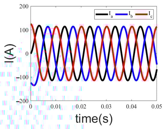
Figure 5.
Normal Three phase current.
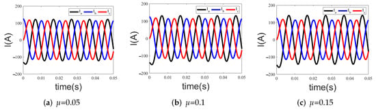
Figure 6.
Three phase current when there is an A−phase fault. (a) = 0.05 (b) = 0.1 (c) = 0.15.
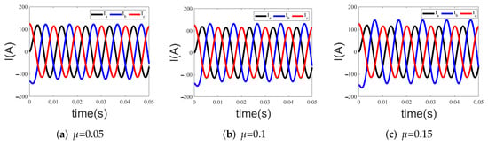
Figure 7.
Three phase current when there is a B−phase fault. (a) = 0.05 (b) = 0.1 (c) = 0.15.
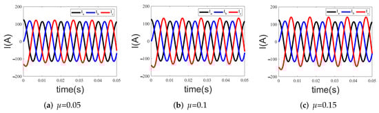
Figure 8.
Three phase current when C−phase fault. (a) = 0.05 (b) = 0.1 (c) = 0.15.
Reference [24] used PSO for optimization, with a total of 30 iterations and 8 particles in each generation. In other words, there are 240 operations, and the relative error of the results is approximately 0.5%. After the improvement of model and cost function, Reference [25], with a total of 30 iterations and 4 particles in each generation and the relative error of the results, is approximately 0.06%. Referring to the above literature and a large number of simulation attempts, the specific parameters of PSO are shown in the Table 1.

Table 1.
The parameters of PSO in the simulation.
In order to ensure the rationality of the simulations, the number of operations is also fixed at 120 in this paper. Because the can be easily found as a discrete value with each methods, we carried out 10 attempts with each method, namely the fault diagnosis method based on PSO, GA, WOA and SPGD, and compared the means and variances of the relative error of . The relative error of is defined as the absolute value of the difference between the preset value of and the estimated value of divided by a preset value of . When is preset to be 0.05, the relative errors of obtained by these four methods of each simulation are shown in Figure 9 and the means and variances of relative error of obtained by these four methods in ten attempts are showed in Table 2. When is preset as 0.1 and 0.15, respectively, the results are shown in Figure 10 and Figure 11, Table 3 and Table 4.
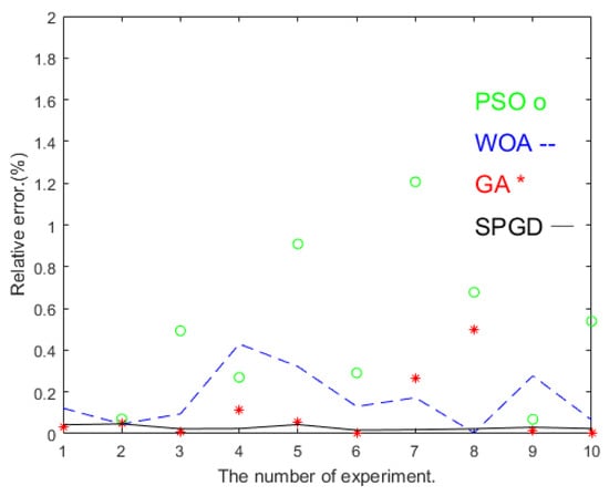
Figure 9.
Comparison of relative error of different methods in 10 experiments when = 0.05.
Table 2.
The mean values and variances of relative error in 10 experiments in different methods when = 0.05.
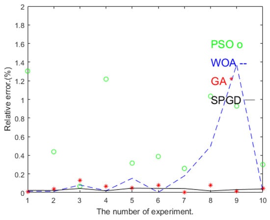
Figure 10.
Comparison of relative error of different methods in 10 experiments when = 0.1.
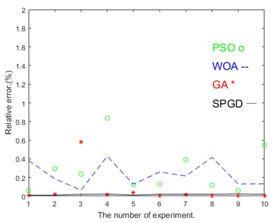
Figure 11.
Comparison of relative error of different methods in 10 experiments when = 0.15.
Table 3.
The mean values and variances of relative error in 10 experiments in different methods when = 0.1.
Table 4.
The mean values and variances of relative error in 10 experiments in different methods when = 0.15.
It can be seen from the results of ten attempts at different that the means of relative error of the obtained by PSO are larger than those of WOA and GA, which indicates that, among these three heuristic algorithms, the precision of evaluating the faulty severity of proposed methods is more satisfactory than that of PSO. Moreover, comparing the means obtained by SPGD with the means obtained by three heuristic algorithms, the method based on SPGD has the most accurate performance for estimating the fault severity. However, compared with the method based on SPGD, it is shown in Figure 8, Figure 9 and Figure 10 that GA can make the smallest value sometimes. However, since the results of GA have a larger fluctuation range than that of SPGD, which is also represented in the values of variances showed in tables, the results of GA are not stable to some extent. In conclusion, from the perspective of means and variances, the method based on SPGD is much better than other methods mentioned above.
Additionally, in order to prove the reliability and rapidity of the fault diagnosis method based on SPGD, the convergence of this method is considered and observed. Since the gradient cannot be obtained for the discrete quantity , in order to ensure the consistency of the number of operations, 40 iterations are carried out for each phase. The assumed short-circuit turns ratios are and . For each phase, the iterative initial value . The variation trend of cost function in faulty phase is shown in Figure 12, and the variation trend of is shown in Figure 13.
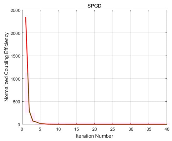
Figure 12.
The variation trend of cost function of SPGD.
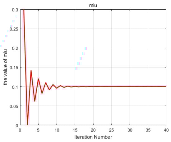
Figure 13.
The variation trend of value of of SPGD.
From the results, it can be demonstrated that the value of the cost function converges to the minimum at a pretty fast speed. After about the fifth iteration, the cost function is basically close to zero, which means that it can rapidly judge whether the ITSC occurs. The estimated value of also converges to the preset short-circuit turns ratio after the 15th iteration, and the final relative error is 0.01%, which denotes that, in addition to fast convergence, favorable accuracy can also be guaranteed.
All in all, the method based on SPGD possesses relatively precise, stable and rapid properties compared with the methods based on the PSO, GA and WOA.
4.2. The Fault Diagnostic Accuracy of the Method Based on SPGD for ITSC Diagnosis under Nonideal Condition
4.2.1. The Fault Diagnostic Accuracy of the Method Based on SPGD in the Case of Input Three Phase Voltage Phase Imbalance
In this section, we set the input three-phase voltage phase at 0, and , respectively, which is imbalanced. Two situations under imbalanced input voltages are considered. One is a situation where the ITSC does not occur and the other is that the ITSC occurs in one phase. For simplicity, we determine the faulty phase is B phase and the ITSC ration is 0.1. The current waveform of the two situations mentioned above as shown in Figure 14. The trend of relative error of is displayed in Figure 15.
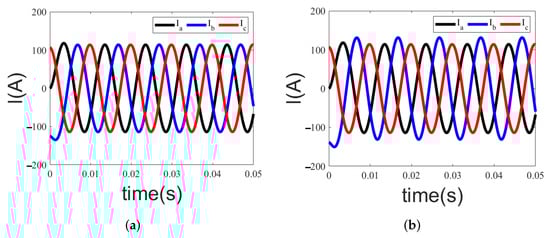
Figure 14.
The current waveform when input voltage phase is imbalanced. (a) Input voltage phase is imbalanced when ITSC fault does not occur; (b) Input voltage phase is imbalanced and = 0.1 in B phase.
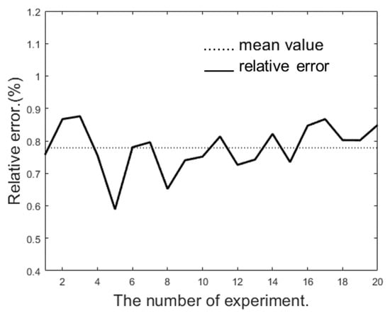
Figure 15.
The relative error when input voltage phase is imbalance.
It can be calculated that the mean value of relative error of is 0.778% in twenty simulations. Although the accuracy is decreased compared with the situation whose input three-phase voltage is symmetric, it is still at a high level. Therefore, when the input three-phase voltage is not balanced strictly, the estimation for the fault severity of proposed method is acceptable.
4.2.2. The Fault Diagnostic Accuracy of the Method Based on SPGD in the Case of Input Three-Phase Voltage Amplitude Imbalance
In this section, in order to verify the robustness of the proposed method when the input voltage’s amplitude is asymmetric, the noise is added to the input three-phase voltage. Two situations under imbalanced input voltage are considered as well. One is the situation where the ITSC does not occur and the other is that the ITSC occurs in one phase. For simplicity, we determine the faulty phase is the B phase and the ITSC ration is 0.1. The current waveform is shown in Figure 16. We also record the trend of the relative error of in 20 simulations, which is shown in Figure 17.
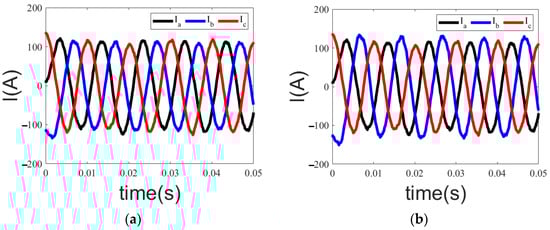
Figure 16.
The current waveform when input voltage phase is imbalance (a) Input voltage amplitude is imbalanced when ITSC fault does not occur; (b) input voltage amplitude is imbalanced and = 0.1 in B phase.
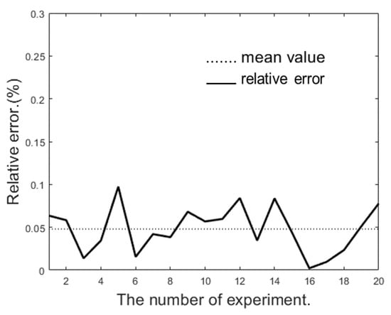
Figure 17.
The relative error when input voltage amplitude is imbalance.
The mean value of the relative error of can be calculated as 0.047%. Compared with the ideal situation, the estimation accuracy is only slightly lower. So the influence of input disturbance, namely the input three-phase voltage being asymmetric, poses a trifling impact on the proposed method, which is suitable for practical engineering.
4.2.3. The Fault Diagnostic Accuracy of Proposed Methods for ITSC Diagnosis under High-Order Harmonics
In the real work environment, there are various high-order harmonics occurring in the stator currents, which will distort the currents and lead to a number of adverse influences. Accordingly, in this section, we conduct some measurement studies under the high-order harmonics at different load moments, which can simulate the motor drive system in practical engineering.
Similarly, we determine that the faulty phase is B phase as well, and the second, third, fifth and seventh harmonics are added in the phase A. The third, fourth, fifth and seventh harmonics are added in phase B. The third, fifth, sixth and seventh harmonics are added in phase C. The stator currents with high-order harmonics are displayed in the Figure 18. In addition, different load moments are taken into consideration, and with a fixed load moment, we run ten attempts and average the values. The specific result is shown in Table 5.
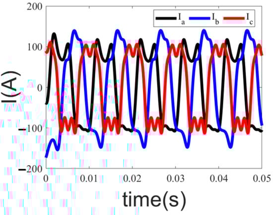
Figure 18.
The waveform under the high−order harmonics.
Table 5.
The relative error of each method under the high-order harmonics at different load moments.
As we can observe in Table 5, the relative errors with high-order harmonics of PSO, GA and WOA at different load moments are all approximately 7%, which is slightly higher than the results without high-order harmonics, but they are still in a very small scope. The relative errors of SPGD are about 6.5% and slightly lower than those of PSO, GA and WOA, which demonstrates that the results of SPGD are better than those of the optimization algorithms mentioned above. However, it illustrates that the high-order harmonics and different load moments do pose a certain effect, but the influences are not particularly serious. The adverse effects caused by high-order harmonics and different load moments affect the SPGD even less. All in all, the proposed methods can still judge the faulty phase of ITSC and estimate the severity index of ITSC with small error to some degree under the undesirable influence of high-order harmonics at different load moments.
5. Experimental Validation
From the above simulation results, it is obvious that the SPGD can achieve the more desired result compared with other optimization algorithms used in this paper. Thus, we only apply the SPGD to verify its effectiveness on the actual PMSM platform. The experiment environment is showed in Figure 19. The specific parameters of the PMSM are as follows. The pole pair p is 2. The phase resistance is . The phase self-inductance is 0.0045 mH. The flux linkage is 0.2 wb. The sampling frequency is 10 KHZ.

Figure 19.
The experiment environment.
In this experiment, the fault severity index is assumed as 0.2. The phase current waveform of the three-phase PMSM is shown in Figure 20. As we can see in Figure 20, compared with the simulation, the waveform is not smooth, which may be caused by the harmonics, equipment loss and so on.
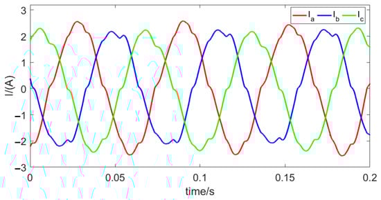
Figure 20.
The waveform under the high−order harmonics.
The experimental result is displayed in Figure 21. As we can see in Figure 21, can be converged into the preset value, which demonstrates that the proposed method can accurately diagnose the faulty severity of the PMSM under the ITSC fault and has certain practical value in real engineering.
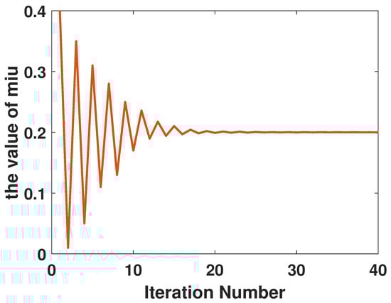
Figure 21.
The waveform under the high−order harmonics.
6. Conclusions
In this paper, aiming at the ITSC fault of PMSM, certain fault diagnosis methods based on heuristic optimization algorithms—that is, the particle swarm optimization algorithm, genetic algorithm and whale optimization algorithm—are proposed. In addition, due to the great random influence of the heuristic algorithm, the stochastic parallel gradient descent algorithm is utilized. This algorithm, i.e., the stochastic parallel gradient descent algorithm, regards the model as a black box and uses random interference to obtain the approximate gradient. In the simulation, the genetic algorithm, whale optimization algorithm and stochastic parallel gradient descent are compared with the existing fault diagnosis method based on particle swarm optimization under ideal circumstances, respectively. The simulation results demonstrate that the performance of proposed methods is promoted a lot. In particular, compared with other heuristic algorithms, the stochastic parallel gradient descent algorithm can acquire more stable diagnosis results with smaller relative error. Moreover, in the case that input three-phase voltage is asymmetric and in the case that high-order harmonics at different load moments are taken into consideration, the method based on stochastic parallel gradient descent still maintains a favorable performance on the fault diagnosis for ITSC, which is applicable for the real engineering. Additionally, from the experimental result, the SPGD can still diagnose the faulty severity.
Author Contributions
Conceptualization, X.C.; methodology, T.Z.; software, Y.C. and W.L.; validation, X.C. and P.Q.; formal analysis, T.Z.; investigation, X.C. and Y.C.; resources, Y.M.; data curation, J.Z.; writing—original draft preparation, W.L. and J.Z.; writing—review and editing, W.L. and P.Q.; visualization, X.C.; supervision, Y.M.; project administration, Y.M. All authors have read and agreed to the published version of the manuscript.
Funding
This research received no external funding.
Institutional Review Board Statement
Not applicable.
Informed Consent Statement
Not applicable.
Data Availability Statement
Not applicable.
Conflicts of Interest
The authors declare no conflict of interest.
References
- Gandhi, A.; Corrigan, T.; Parsa, L. Recent Advances in Modeling and Online Detection of Stator Interturn Faults in Electrical Motors. IEEE Trans. Ind. Electron. 2011, 58, 1564–1575. [Google Scholar] [CrossRef]
- Leboeuf, N.; Boileau, T.; Nahid-Mobarakeh, B.; Clerc, G.; Meibody-Tabar, F. Real-Time Detection of Interturn Faults in PM Drives Using Back-EMF Estimation and Residual Analysis. IEEE Trans. Ind. Appl. 2011, 47, 2402–2412. [Google Scholar] [CrossRef]
- Sarikhani, A.; Mohammed, O.A. Inter-Turn Fault Detection in PM Synchronous Machines by Physics-Based Back Electromotive Force Estimation. IEEE Trans. Ind. Electron. 2013, 60, 3472–3484. [Google Scholar] [CrossRef]
- Boileau, T.; Nahid-Mobarakeh, B.; Meibody-Tabar, F. Back-EMF Based Detection of Stator Winding Inter-turn Fault for PM Synchronous Motor Drives. In Proceedings of the Vehicle Power & Propulsion Conference, Arlington, TX, USA, 9–12 September 2007; pp. 95–100. [Google Scholar]
- Krolczyk, G.M.; Krolczyk, J.B.; Legutko, S.; Hunjet, A. Effect of the disc processing technology on the vibration level of the chipper during operations. Teh. Vjesn. 2014, 447–450. [Google Scholar]
- Capolino, G.A.; Henao, H.; Demian, C. A frequency-domain detection of stator winding faults in induction machines using an external flux sensor. In Proceedings of the Industry Applications Conference, Salt Lake City, CA, USA, 12–16 October 2003. [Google Scholar]
- Cira, F.; Arkan, M.; Gumus, B.; Goktas, T. Analysis of stator inter-turn short-circuit fault signatures for inverter-fed permanent magnet synchronous motors. In Proceedings of the IECON 2016-42nd Annual Conference of the IEEE Industrial Electronics Society, Florence, Italy, 24–27 October 2016. [Google Scholar]
- Ping, Z.A.; Yang, J.; Ling, W. Fault Detection of Stator Winding Interturn Short Circuit in PMSM Based on Wavelet Packet Analysis. In Proceedings of the Fifth International Conference on Measuring Technology & Mechatronics Automation, Hong Kong, China, 16–17 January 2013. [Google Scholar]
- Moosavi, S.S.; Esmaili, Q.; Djerdir, A.; Amirat, Y.A. Inter-Turn Fault Detection in Stator Winding of PMSM Using Wavelet Transform. In Proceedings of the 2017 IEEE Vehicle Power and Propulsion Conference (VPPC), Belfort, France, 14–17 December 2017. [Google Scholar]
- Obeid, N.H.; Boileau, T.; Nahid-Mobarakeh, B. Modeling and diagnostic of incipient inter-turn faults for a three phase permanent magnet synchronous motor using wavelet transform. In Proceedings of the 2014 IEEE Industry Applications Society Annual Meeting, Las Vegas, NV, USA, 7–11 October 2015. [Google Scholar]
- Gao, Z.; Cecati, C.; Ding, S.X. A Survey of Fault Diagnosis and Fault-Tolerant Techniques—Part II: Fault Diagnosis With Knowledge-Based and Hybrid/Active Approaches. IEEE Trans. Ind. Electron. 2015, 62, 3768–3774. [Google Scholar] [CrossRef] [Green Version]
- Quiroga, J.; Liu, L.; Cartes, D.A. Fuzzy logic based fault detection of PMSM stator winding short under load fluctuation using negative sequence analysis. In Proceedings of the American Control Conference, Seattle, WA, USA, 11–13 June 2008; pp. 4262–4267. [Google Scholar]
- Liang, S.; Chen, Y.; Liang, H.; Li, X. Sparse Representation and SVM Diagnosis Method for Inter-Turn Short-Circuit Fault in PMSM. Appl. Sci. 2019, 9, 224. [Google Scholar] [CrossRef] [Green Version]
- Das, S.; Koley, C.; Purkait, P.; Chakravorti, S. Wavelet aided SVM classifier for stator inter-turn fault monitoring in induction motors. In Proceedings of the Power & Energy Society General Meeting IEEE 2010, Minneapolis, MN, USA, 25–29 July 2010. [Google Scholar]
- Nyanteh, Y.; Edrington, C.; Srivastava, S.; Cartes, D. Application of Artificial Intelligence to Real-Time Fault Detection in Permanent-Magnet Synchronous Machines. IEEE Trans. Ind. Appl. 2013, 49, 1205–1214. [Google Scholar] [CrossRef]
- Vaseghi, B.; Takorabet, N.; Meibody-Ta Ba R, F.; Djerdir, A.; Farooq, J.A.; Miraoui, A. Modeling and characterizing the inter-turn short circuit fault in PMSM. In Proceedings of the 2011 IEEE International Electric Machines & Drives Conference (IEMDC), Niagara Falls, ON, Canada, 15–18 May 2011. [Google Scholar]
- Yang, J.W.; Dai, Z.Y.; Zhang, Z. Modeling and fault diagnosis of multi-phase winding inter-turn short circuit for five-phase PMSM based on improved trust region-ScienceDirect. Microelectron. Reliab. 2020, 114, 113778. [Google Scholar] [CrossRef]
- Liu, W.; Li, L.; Chung, I.Y.; Cartes, D.A.; Wei, Z. Modeling and detecting the stator winding fault of permanent magnet synchronous motors. Simul. Model. Pract. Theory 2012, 27, 1–16. [Google Scholar] [CrossRef]
- Eberhart, R.; Kennedy, J. New optimizer using particle swarm theory. In Proceedings of the International Symposium on Micro Machine and Human Science, Nagoya, Japan, 4–6 October 1995; pp. 39–43. [Google Scholar]
- Kennedy, J.; Eberhart, R.C. A discrete binary version of the particle swarm algorithm. In Proceedings of the 1997 IEEE International Conference on Systems, Man, and Cybernetics. Computational Cybernetics and Simulation, Orlando, FL, USA, 12–15 October 1997. [Google Scholar]
- Mirjalili, S.; Lewis, A. The Whale Optimization Algorithm. Adv. Eng. Softw. 2016, 95, 51–67. [Google Scholar] [CrossRef]
- Vorontsov, M.A.; Sivokon, V.P. Stochastic parallel-gradient-descent technique for high-resolution wave-front phase-distortion correction. J. Opt. Soc. Am. A 1998, 15, 2745–2758. [Google Scholar] [CrossRef]
- Dang, Z. Study on Fault Diagnosis and Fault Tolerant Control of Permanent Magnet Synchronous Motor interturn Short Circuit. Ph.D. Thesis, Xi’an University of Science and Technology, Xi’an, China, 2020. [Google Scholar]
- Li, L.; Cartes, D.A.; Liu, W. Application of Particle Swarm Optimization to PMSM Stator Fault Diagnosis. In Proceedings of the 2006 IEEE International Joint Conference on Neural Network Proceedings, Vancouver, BC, Canada, 16–21 July 2006. [Google Scholar]
- Grouz, F.; Sbita, L.; Boussak, M. Particle swarm optimization based fault diagnosis for non-salient PMSM with multi-phase inter-turn short circuit. In Proceedings of the International Conference on Communications, Computing and Control Applications (CCCA) CCCA12, Marseilles, France, 6–8 December 2012. [Google Scholar]
Publisher’s Note: MDPI stays neutral with regard to jurisdictional claims in published maps and institutional affiliations. |
© 2022 by the authors. Licensee MDPI, Basel, Switzerland. This article is an open access article distributed under the terms and conditions of the Creative Commons Attribution (CC BY) license (https://creativecommons.org/licenses/by/4.0/).