Abstract
Interpolating trajectories of points and geometric entities is an important problem for kinematics. To describe these trajectories, several algorithms have been proposed using matrices, quaternions, dual-quaternions, and the Study quadric; the last one allows the embedding of motors as 8D vectors into projective space , where the interpolation of rotations and translations becomes a linear problem. Furthermore, conformal geometric algebra (CGA) is an effective and intuitive framework for representing and manipulating geometric entities in Euclidean spaces, and it allows the use of quaternions and dual-quaternions formulated as Motors. In this paper, a new methodology for accelerating the Study quadric Interpolation based on Conformal Geometric Algebra is presented. This methodology uses General Purpose Graphics Processing Units (GPUs) and it is applied for medical robotics, but it can also be extended to other areas such as aeronautics, robotics, and graphics processing.
1. Introduction
Generating trajectories for 3D objects is a fundamental problem in areas of robotics, image processing, and others. There are few mathematical algorithms for the interpolation of points that use vector calculus, quaternions, dual-quaternions, and linear algebra. Geometric algebra is a powerful mathematical framework for solving problems using basic geometry entities (circles, points, spheres, planes, and lines), and can represent Euclidean geometry, quaternions, and dual-quaternions. For this reason, it can be used for interpolating geometric entities for applications in medical robotics, graphic engineering, robotics, and aeronautics.
In screw theory, Chasles’ theorem states that a general displacement can be represented using a screw motion (cylindrical helix). Screw theory is widely used in mechanics and robotics and linear interpolation is the simple manner for interpolation; however, screw theory allows many other forms of interpolation, such as Bézier curves [1] or three-point quadratic. The pure rotation interpolation reduces exactly to the rotor or quaternionic SO(3) Lie group interpolation. In this paper, we propose the Study quadratic interpolation using the motor algebra for the SE(3) Lie group; a sub-algebra of the conformal geometric algebra.
This work focuses on the reformulation of the quadric Study interpolation method in conformal geometric algebra. The work shows that the speed up of the quadratic interpolation using GPU improves the algorithm’s performance significantly. These results are not surprising, since the replacement of matrices with geometric algebra formulations are known to be superior in numerical stability and performance; also, using GPU hardware is generally faster than CPUs.
The contribution of this work is as follows:
- Formulation of the quadratic interpolation algorithm using motors of conformal geometric algebra as 8D vectors in the Study manifold;
- Speeding up the quadratic interpolation algorithm using GPU;
- Comparison of fast quadratic interpolation GPU versus CPU;
- The interpolation of the motion of geometric objects in conformal geometric algebra;
- Application of the interpolation algorithm in kidney surgery.
This paper is organized as follows: Section 2 reports on related work, Section 3 gives a brief introduction to geometric algebra, with special emphasis on conformal geometric algebra. Section 4 describe the rigid motion and similitude group interpolation methods. Section 5 explains the interpolation algorithm using the Study Quadric Manifod. Section 6 describes the speeding up the algorithms using a GPU accelerator. Section 7 shows the experimental results. Section 8 shows an example of interpolation of motion in surgery. Finally, Section 9 presents our conclusions and future work.
2. Related Work
Due to the easy representation of complex problems in robotics and image processing, several works have been proposed to accelerate geometric algebra operations. Most related techniques for accelerating geometric algebra algorithms are based on speeding up basic operations (inner, outer and geometric product, etc.) with FPGA Co-processors [2,3,4,5] and GPU parallelization [6,7].
More complex architectures have been developed for applications on computational vision. In [8], the authors present an algorithm of Clifford convolution and Clifford Fourier transforms for color edge detection, and an alternative algorithm based on rotor edge detection is proposed in [9]. Gerardo Soria-García et al. introduce an FPGA implementation of a Conformal Geometric Algebra Voting Scheme for Geometric Entities Extraction, such as lines and circles on images of edges [10].
A GPU implementation for a conformal geometric algebra interpolation application based on GPU is presented in [11]. The algorithm presented in this work is a modification using motors of the dual-quaternion method to interpolate rotation, translation, and dilation of geometric entities such as points, lines, circles, , planes, and spheres.
Recently, the following authors have produced highly optimized code for GA algorithms: D. Hildenbrand developed the GAALOP code generator for GA algorithms with optimized output on various CPUs and GPUs [6,12]; and Ahmed Eid’ developed the geometric algebra package GMac [13,14,15].
In our work, we focus on the direct implementation of the Study quadric interpolation optimizing the source code for a better execution in the GPU, that is, we reduce the complexity of our source code in order to suit to a computation via the GPU. If a user wants, on top of that, to use code generators like GAALOP or GMac, it would of course reduce the complexity even more.
3. Geometric Algebra
In an n-dimensional real vector space , we can introduce an orthonormal basis of vectors , for . This leads to a basis for the entire geometric algebra:
The Geometric Algebra (GA) of the real n-dimensional quadratic vector space is denoted as . In the case of the notation , () denotes the GA of where correspond to the number of basis vectors which square in GA to 1, −1 or 0; that is, , , and , respectively. When a unit vector squares to 0, it is seen as a null vector as in the motor algebra or the point at the origin or at infinity which squares to zero.
In the cases when , or for simplicity, we denote , respectively. If only , we denote .
Definition 1.
The geometric product of two vectors a and b is written as and it is expressed as a sum of its symmetric and antisymmetric parts:
is a graded linear space:
where the elements of are referred to as (homogeneous) multivectors of grad k for . In the following, for short, elements of are called vectors. Thus, any can be uniquely decomposed into a sum where .
Furthermore, is a -graded algebra in the following sense:
where
Then, (resp. ) is called the even (resp. the odd) part pf . Note that, due to Equation (4), is a subalgebra of . Later in this paper, the even subalgebra of will be denoted by .
The dimension of is . The multivector basis of has bases for scalars, bivectors, trivectors and k-vectors. A k-blade is either the identity element 1 of (when k = 0 or, when k> 0), it is defined as the wedge product . A linear combination of k-vectors is called a homogeneous multivector.
Consider two homogeneous multivectors and of grades r and s, respectively. The geometric product of and can be written as:
Multivector computing involving inner products is easier if one employs the next equality for the generalized inner product of two blades , and :
For , use the following equation:
and for
From these equations, we can see that the inner product is not commutative for general multivectors.
3.1. Conformal Geometric Algebra
In Conformal Geometric Algebra (CGA), the Euclidean vector space is represented in . The space for has an orthonormal vector basis given by with the properties , , , .
The null basis (origin and point at infinity) is defined as:
These null vectors satisfy the relations and .
Let be the Minkowski plane. The unit Euclidean pseudo-scalar is , and the conformal pseudoscalar is used for computing the inverse and duals of multivectors. Given a nonsingular k-vector , the dual and its inverse are, respectively,
where stands for the reversion of A and its magnitude.
3.2. Points, Lines, Planes, and Spheres
The representation of a 3D Euclidean point x, y, z in the geometric algebra is given by:
According to Equation (7), given two conformal points and , their difference in Euclidean space can be computed as follows:
and, consequently, the following equality:
is fulfilled as well.
The line is formulated as a form in the Inner Product Null Space (IPNS) as follows:
where n (bivector) is the orientation and the vector m is the moment of the line.
The plane is formulated as a form in IPNS
where the n (bivector) for the plane orientation and d is the distance from origin orthogonal to the plane.
The sphere is formulated as a form in IPNS:
A point is a sphere with zero radius. Considering the dual equation for the sphere, we can write the constraint for a point lying on a sphere:
The sphere can be directly computed by the wedge of four conformal points in the Outer Product Null Space (OPNS):
Replacing any of these points with the point at infinity, we obtain the OPNS plane equation:
Similar to Equation (20), the OPNS line equation can be formulated as a circle passing through the point at infinity:
see in Table 1 the summary of the IPNS and OPNS geometric objects.

Table 1.
Geometric entities in conformal geometric algebra. The IPNS and OPNS stand for Inner Product Null Space and Outer Product Null Space respectively.
3.3. Rigid Transformations
In CGA many of the transformations can be formulated in terms of successive reflections between planes.
3.3.1. Reflection
The equation of a point x reflected with respect to a plane is:
3.3.2. Translation
The transformation of geometric entity O formulated as two successive reflections w.r.t. the parallel planes and is given by:
where , d is the distance of translation, and n is the direction of translation.
3.3.3. Rotation
Similarly, we can formulate a rotation as the product of two reflections between non-parallel planes and which cross the origin.
The geometric product of the unit normal vectors of these planes and yields the equation for the rotor:
where the unit bivector , and the angle is twice the angle between and .
3.3.4. Screw Motion
The operator for screw motion or motor M is a composition of a translator T and a rotor R, both w.r.t. to an arbitrary axis L. The equation for a motor is as follows:
where the screw line is ; n and m stand for the orientation and momentum of the screw line and the dual angle . Finally, the motor transformation for any object reads
4. Rigid Motion and Similitude Group Interpolation
This section presents the motor interpolation. We will use this technique when we interpolate geometric objects like points, lines, planes, circles and spheres.
This is a generalization of the well known Spherical Linear Interpolation (SLERP) method [16] Given and two motors representing the initial and final pose of a rigid body respectively, the Motor Spherical Linear Interpolation function (MSLERP) is defined as follows
with . The underlying kinematic concept of the screw motion was explained in previous sections. A kinematic explanation of this interpolation method was given by [16,17]. Since represents the finite screw motion between the initial and final pose of the rigid body, specifically the product:
defines a screw motion of a dual angle along the screw axis . In this equation, and t stand for the rotation angle and the translation bivector, respectively.
The Motor Linear Blending interpolation method (MLB) is defined as follows:
This procedure can be extended to the interpolation involving several poses:
These weights are assumed to be convex, namely and . One can choose weights that are made coincident with the coefficients of the classical Lagrange’s interpolating polynomials
Note that Algorithm 1 uses the resulting bivector B (se(3) Lie algebra) to compute the motor (SE(3) Lie group). To interpolate geometric objects O in the conformal geometric algebra framework, represented in IPNS, as points in Equation (12), lines in Equation (15), planes in Equation (16) and spheres in Equation (16), we represent the objects using an IPNS representation and apply the blending interpolated motor and for spheres a Dilator as well,
| Algorithm 1 MIB: Motor Iterative Blending. |
|
5. Interpolation Algorithm Using the Study Quadric Manifold
According Gfrerrer [18], one can formulate an interpolation algorithm using the Study’s kinematics mapping.This maps Euclidean rigid transformations into homogeneous points which in turn belong to the Study quadric (projective space )
where is the special Lie group for 3D Euclidean rigid transformations, represents any Euclidean rigid transformation and the vector X containing homogeneous coordinates . Note that the motor algebra is a sub-algebra of the 3D conformal geometric algebra , thus the interpolation uses motors, depending upon which algebra is used one can use I for motors of or for motors of which both square to zero and are acting similarly to the isotropic operator of the dual quaternions, which use , which squares to zero as well.
Given the set containing three homogeneous points , that is, these points lie on a manifold , which is embedded in the projective space (). The interpolation curve is generated by interpolating the given homogeneous points which satisfy the set computed as follows
This equation represents a discretization of the curve into N points. i.e., intermediate points are computed.
The interpolation polynomials , , and are formulated as follows
where t, , , and are interpolation values between 0 and 1. t represents the segment of curve where the point is calculated, , and are values that represent the section of curve where interpolated and control points meet. The algorithm checks the number of elements in X, if there is only one point, this is returned as the solution, otherwise, X is used to get intermediate control points via Equation (38) and saved in M. For N control points, we obtain interpolation points.
The Study-quadric bilinear form is given by the following matrix ,
If one wishes to interpolate more points, the above-explained interpolation equation can be extended and adapted as De Casteljau’s algorithm [19]. This is shown in Algorithm 2.
This algorithm calculates a homogeneous point for the given set that contains the control points () and the interpolation values () and the Study quadric bilinear matrix . Here are interpolation variables. t is the position interval variable and allows us to determine the position within the curve of the interpolation point, the value t goes from 0 to 1. To calculate all the points of the curve, all the values of t are traversed. are values that indicate at which point the interpolation points, in the functions that came in the Klawiter library [19], the values , are proposed so that the interpolated points correspond to the initial control point, the mid-control point and the endpoint, respectively. These are fixed for each curve, only t is what can change when calculating a point within a specific curve. In the algorithm, the triple of the set of points will be selected as follows: for .
The algorithm checks the number of elements in . If there is only one point, this is returned as the solution. Otherwise, is used to obtain intermediate control points via Equation (38) and saved in . is used to call the algorithm recursively until we get only one interpolation point and return it. Figure 1 shows the algorithm interpolation for five control points. See that, in each interpolation step, for N control points, we get interpolation points and repeats are required. Since in the last step, Equation (38) required three points, an odd number of control points is needed. \
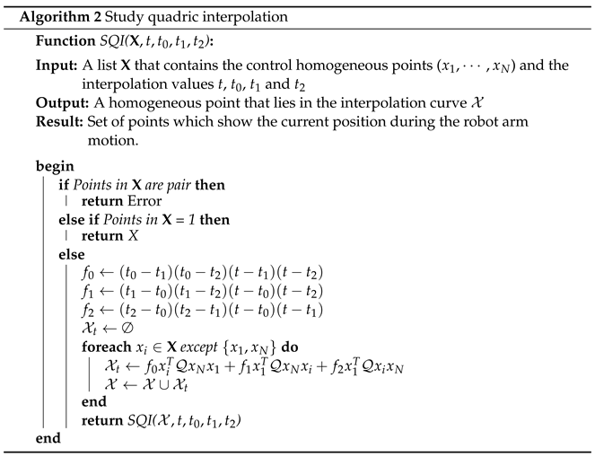
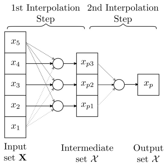
Figure 1.
Interpolation of five control points with Algorithm 2.
Where is the set of control homogeneous points () that describe the discrete curve trajectory, is the quadric matrix, , , and are global constant values, in this case, 0, and 1 respectively. As is seen in the algorithm, it is required that the array X has an odd number of homogeneous points to get an interpolation curve. Note that the solution is in fact a rational motion utilizing an interpolating spline which in turn involves rational sub-spline motions, see [1].
In general, the Study quadric interpolation algorithm uses homogeneous points represented by dual-quaternions or by homogenous matrices. As we know, motors are isomorphic to dual-quaternions and a motor can be represented as a homogeneous point as well. This motor represented as a vector lies on the Study Manifold (see Table 2). In this regard, we propose a modified interpolation algorithm. For that, the homogeneous points are replaced by motors and matrix operations are substituted with GA operations.
Table 2.
Study quadric homogeneous point represented in dual-quaternion and its equivalences as a motor in and as a motor in .
Since the matrix multiplications in (38) with the form , the result of which is a constant value expressed as:
Changing the homogeneous points with their respective motor representations in CGA and analyzing the motor multiplication, is shown that the coefficient of the blade () from the motor multiplication is the double value of (41). This coefficient () can be extracted from any motor using the partial derivative:
or via the inner product with the and :
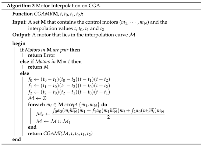
Using GA, Equation (38) is reformulated for a motor based interpolation algorithm. It uses three control motors as follows:
In the same manner as in Algorithm 2, for more control points, Equation (44) can be rewritten using the De Casteljau’s algorithm as described in Algorithm 3. This algorithm calculates one motor for the set of control motors () and the interpolation constants (t,,,). Similar to Algorithm 2, the interpolation function is called recursively with the calculated motors from the last step as an input until we get only one motor. Since the last step needs three motors to calculate the last one, must contain an odd number of motors.
6. Speeding up the Algorithms Using a GPU Accelerator
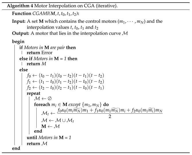
To implement the motor interpolation, we translated the Algorithm 3 into an equivalent-iterative version given by Algorithm 4; for more detail technical aspects see [20].
The GPU and CPU have different architectures. The CPU has a few sets of cores for sequential applications. In contrast, the GPU has many cores for highly parallel computing. Figure 2 compares the CPU and GPU architectures. Note that GPU cores run asynchronously using threads. Each core is limited to 32, 64, 128, 256, or 512 threads. If a parallel GPU implementation is launched, a certain number of cores are required. These are figured out as a direct function of the selected threads per block. In the case of the motor interpolation, each thread launches a copy of the algorithm.
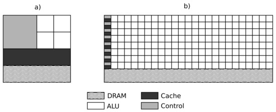
Figure 2.
Architecture comparison of (a) CPU and (b) GPU.
All GPU operations run explicitly or implicitly on a stream, where multiple streams are launched and the transference data and kernel launch can be overlapped as shown in Figure 3; for more detail technical aspects see [20].
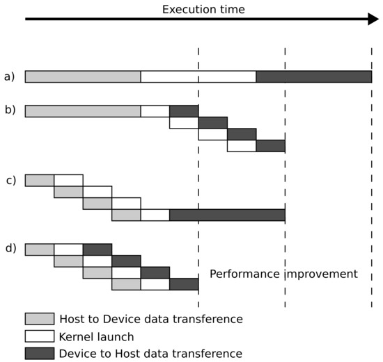
Figure 3.
Different streams used for a concurrent implementation (a) 1-stream, (b) concurrent approach for a device-to-host asynchronous memory copy, (c) concurrent approach for host-to-device asynchronous memory copy, (d) concurrent approach for host-to-device and device-to-host asynchronous memory copy.
For the case of the parallel calculation of multiple curves, the multi-streaming implementation is used and each curve is computed in an independent stream.
7. Experiments
7.1. Interpolation of the Motion of Geometric Entities
The interpolation motors can be used to calculate the new position of geometric entities as follows:
where can be, at instant i, any geometric entity of point, line, plane, circle, sphere or point pairs expressed in conformal geometric algebra [21]. Figure 4 shows the interpolation of these geometric objects under the action of a motor .
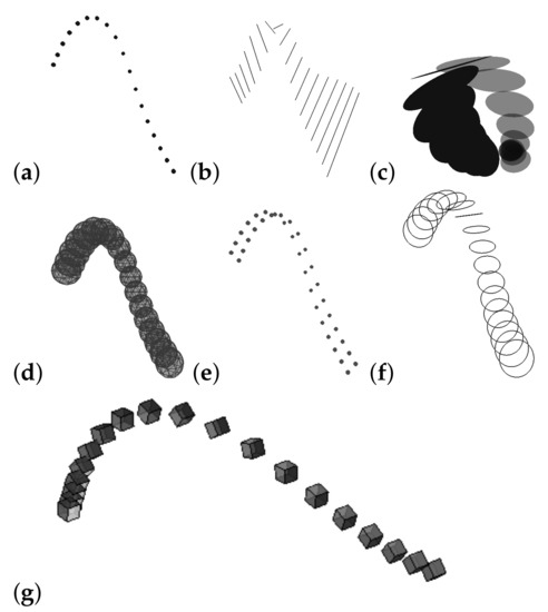
Figure 4.
Interpolation of geometric entities : (a) points, (b) lines, (c) planes, (d) spheres, (e) point pairs, and (f) circles using the CGA motor interpolation curve (g).
7.2. Speeding up the Algorithms Using a GPU Accelerator
The Study’s quadric and the motor interpolation are compared to analyze which of the algorithms has the best speed performance. The results are presented in Figure 5. We see that the motor interpolation version is faster than the Study quadric interpolation, namely for 20,000 points, it is 28× times faster.
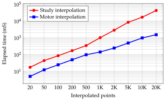
Figure 5.
Comparison of Study’s quadric and Motor interpolation speed-up.
Figure 5 shows that the motor interpolation algorithm selected for sequential and parallel implementation utilizes the same hardware parameters.
The sequential implementation was programmed using C++ language and CUDA C++ for the parallel approach using 32 threads per block in the kernel. The interpolated motors were computed using single and double-precision floating-point representation. All the measures consider only the algorithm execution, but data transference, file writing, and reading are excluded. The results are shown in Figure 6; for a discussion in more detail, see [20].
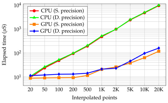
Figure 6.
CPU and GPU speed-up analysis.
It was confirmed that the GPU has the best time performance for calculating the interpolation algorithm. When the time execution in CPU increases linearly, the time in GPU for 500 or fewer points remains almost constant. For the case of 20,000 motors, the GPU implementation runs 79× and 60× times faster than the CPU for single and double floating-point respectively. The different multi-streaming implementations were analyzed; 16 different interpolation curves were calculated using the concurrent approach for host-to-device and device-to-host asynchronous memory copy with 4 configurations (1, 2, 4, and 8 streams) with 32 threads per block. The measure times include data transference. Figure 7 depicts that the use of multi-streaming reduces the execution time considerably, i.e., for 20,000 points, 8 streams version is 2.7×, 1.9× and 1.6× times faster than 1, 2 and 4 streams respectively.
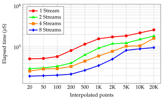
Figure 7.
Comparison of the Multi-Stream speed-up.
8. Interpolation of Surgery Motion
Since this work focuses on the reformulation of the quadric Study interpolation method in conformal geometric algebra and the speed up of the quadratic interpolation using GPU. In this section, we present just an application of the quadratic Study interpolation algorithm. We do not intend to analyze the impact of the quadratic Study interpolation in robotics; this is a goal of our future article.
This Study’s quadric-based motor interpolation was used to interpolate trajectories in medical robotics for kidney surgery, see Figure 8. The robot manipulator has to follow a path for sutureingaround a certain region on the kidney phantom. We design to tasks: follow an UltraSound (US)-probe trajectory and the interpolation of a given 3D points sequence. One provides the point coordinates and their desired orientations; these are interpolated by the motor algorithm (see Figure 8b–d). Afterwards, we check the precision error using inverse kinematics. The inverse kinematics was also formulated in conformal geometric algebra; the algorithm was reported in [21].
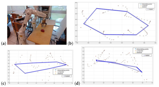
Figure 8.
(a) robot; views: (b) X-Y, (c) X-Z, (d) Y-Z.
9. Conclusions
The interpolation of the trajectory of points and geometric entities is an important problem for kinematics. To describe these trajectories, several algorithms have been proposed using matrices, quaternions, dual-quaternions and the Study quadric. We show that Conformal geometric algebra is an effective and intuitive framework for representing and manipulating the motors as 8D vectors in projective space , where the interpolation of rotations and translations becomes a linear problem. This methodology uses general purpose GPUs and it is applied for medical robotics. In the future, we will pursue implementing the interpolation algorithm using multiple GPUs and reducing the data dependency. We will also build an OpenCL library of the algorithms using Python.
Author Contributions
Conceptualization, E.B.-C., G.M.-T.; methodology, E.B.-C., G.M.-T., S.O.-C.; software, O.U.-P.; validation, G.M.-T., O.U.-P. and G.S.-G.; writing—review and editing, G.M.-T. and E.B.-C.; funding acquisition, E.B.-C. All authors have read and agreed to the published version of the manuscript.
Funding
This work was supported by Mexican CONACYT Project A1-S-10412.
Conflicts of Interest
The authors declare no conflict of interest.
References
- Prautzsch, H.; Boehm, W.; Paluszny, M. Bézier and B-Spline Techniques; Springer Science & Business Media: Berlin, Germany, 2013. [Google Scholar]
- Franchini, S.; Gentile, A.; Sorbello, F.; Vassallo, G.; Vitabile, S. An FPGA implementation of a quadruple-based multiplier for 4D Clifford algebra. In Proceedings of the IEEE 11th EUROMICRO Conference on Digital System Design: Architectures, Methods and Tools 2008 (DSD’08), Parma, Italy, 3–5 September 2008; pp. 743–751. [Google Scholar]
- Franchini, S.; Gentile, A.; Sorbello, F.; Vassallo, G.; Vitabile, S. A New Embedded Coprocessor for Clifford Algebra Based Software Intensive Systems. In Proceedings of the IEEE 2011 International Conference on Complex, Intelligent, and Software Intensive Systems (CISIS), Seoul, Korea, 30 June–2 July 2011; pp. 335–342. [Google Scholar]
- Franchini, S.; Gentile, A.; Sorbello, F.; Vassallo, G.; Vitabile, S. Design and implementation of an embedded coprocessor with native support for 5D, quadruple-based Clifford algebra. IEEE Trans. Comput. 2013, 62, 2366–2381. [Google Scholar] [CrossRef]
- Franchini, S.; Gentile, A.; Sorbello, F.; Vassallo, G.; Vitabile, S. ConformalALU: A conformal geometric algebra coprocessor for medical image processing. IEEE Trans. Comput. 2015, 64, 955–970. [Google Scholar] [CrossRef]
- Lange, H.; Stock, F.; Koch, A.; Hildenbrand, D. Acceleration and energy efficiency of a geometric algebra computation using reconfigurable computers and GPUs. In Proceedings of the IEEE FCCM’09 17th IEEE Symposium on Field Programmable Custom Computing Machines, Napa, CA, USA, 5–7 April 2009; pp. 255–258. [Google Scholar]
- Franchini, S.; Gentile, A.; Vassallo, G.; Vitabile, S. Accelerating Clifford Algebra Operations Using GPUs and an OpenCL Code Generator. In Proceedings of the IEEE 2015 Euromicro Conference on Digital System Design, Madeira, Portugal, 26–28 August 2015; pp. 57–64. [Google Scholar]
- Franchini, S.; Gentile, A.; Vassallo, G.; Sorbello, F.; Vitabile, S. A specialized architecture for color image edge detection based on Clifford algebra. In Proceedings of the IEEE Complex, Intelligent, 2013 Seventh International Conference Complex, Intelligent, and Software Intensive Systems (CISIS), Taichung, Taiwan, 3–5 July 2013; pp. 128–135. [Google Scholar]
- Mishra, B.; Wilson, P. Color edge detection hardware based on geometric algebra. In Proceedings of the 3rd European Conference on Visual Media Production (CVMP 2006) Part of the 2nd Multimedia Conference 2006, IET, London, UK, 29–30 November 2006; pp. 115–121. [Google Scholar]
- Soria-García, G.; Altamirano-Gómez, G.; Ortega-Cisneros, S.; Bayro-Corrochano, E. Conformal Geometric Algebra Voting Scheme implemented in reconfigurable devices for geometric entities extraction. In Proceedings of the IEEE Transactions on Industrial Electronics, Atlanta, GA, USA, 15–17 October 2007; pp. 8747–8755. [Google Scholar]
- Papaefthymiou, M.; Hildenbrand, D.; Papagiannakis, G. An inclusive Conformal Geometric Algebra GPU animation interpolation and deformation algorithm. Vis. Comput. 2016, 32, 751–759. [Google Scholar] [CrossRef]
- Accelerator for GA Computing. Available online: http://www.gaalop.de/D.Hildebrand (accessed on 5 August 2021).
- Eid, A. (Ed.) Code Generation for Geometric Algebra: Combining Geometric, Algebraic, and Software Abstractions for Scientific Computations; Noor Publishing: Chisinau, Moldova, 2016. [Google Scholar]
- Eid, A. Geometric Algebra Packet GMac. Available online: https://github.com/ga-explorer/GMac (accessed on 10 September 2021).
- Eid, A.H. An Extended Implementation Framework for Geometric Algebra Operations on Systems of Coordinate Frames of Arbitrary Signature. Adv. Appl. Clifford Algebr. 2018, 28, 16. [Google Scholar] [CrossRef]
- Etzel, K.R.; McCarthy, J.M. Spatial motion interpolation in an image space of so(4). In Proceedings of the 1996 ASME Design Engineering Technical Conference and Computers in Engineering Conference, Irvine, CA, USA, 18–22 August 1996. [Google Scholar]
- Kavan, L.; Collins, S.; Zara, J.; O’Sullivan, C. Geometric Skinning with Approximate Dual Quaternion Blending; Technical Report TCD-CS-2006-46; The University of Dublin, Trinity College: Dublin, Ireland, 2006. [Google Scholar]
- Gfrerrer, A. Study’s Kinematic Mapping—A Tool for Motion Design. In Advances in Robot Kinematics; Springer: Heidelberg, Germany, 2010; pp. 7–16. [Google Scholar]
- Klawitter, D. Documentation-Kinematic Toolbox; Internal Report; Technische Universität Dresden: Dresden, Germany, 2010. [Google Scholar]
- Bayro-Corrochano, E. (Ed.) Geometric Algebra Applicationsa Vol.II: Robot Modelling and Control; Springer: Heidelberg, Germany, 2020. [Google Scholar]
- Bayro-Corrochano, E. Geometric Computing for Wavelets Transforms, Robot Vision, Learning, Control and Action; Springer: Heidelberg, Germany, 2010. [Google Scholar]
Publisher’s Note: MDPI stays neutral with regard to jurisdictional claims in published maps and institutional affiliations. |
© 2022 by the authors. Licensee MDPI, Basel, Switzerland. This article is an open access article distributed under the terms and conditions of the Creative Commons Attribution (CC BY) license (https://creativecommons.org/licenses/by/4.0/).