Two Advanced Models of the Function of MRT Public Transportation in Taipei

Abstract

Tour traffic prediction is very important in determining the capacity of public transportation and planning new transportation devices, allowing them to be built in accordance with people’s basic needs. From a review of a limited number of studies, the common methods for forecasting tour traffic demand appear to be regression analysis, econometric modeling, time-series modeling, artificial neural networks, and gray theory. In this study, a two-step procedure is used to build a predictive model for public transport. In the first step of this study, regression analysis is used to find the correlations between two or more variables and their associated directions and strength, and the regression function is used to predict future changes. In the second step, the regression analysis and artificial neural network methods are assessed and the results are compared. The artificial neural network is more accurate in prediction than regression analysis. The study results can provide useful references for transportation organizations in the development of business operation strategies for managing sustainable smart cities.

1. Introduction

Taipei has the highest population density and traffic capacity in Taiwan. The construction of the Mass Rapid Transit (MRT) [1] system has relieved long-standing traffic problems in Taipei’s urban area. In addition to its safety and convenience, the public MRT may also control the growth of private vehicles, reduce carbon emissions, and save energy, allowing for the creation of a low-carbon and green energy-based city. The preliminary road network of the public MRT system in the urban area of Taipei was approved by the Executive Yuan in 1986. The Taipei City Government established the Department of Rapid Transit Systems in 1987 and launched the construction of a preliminary road network or extension, following a revision. Taipei Rapid Transit Corporation was incorporated in 1994. The Muzha Line, the first driverless medium-capacity rapid transit line in Taiwan, was opened in March 1996, turning over a new leaf for public transportation in Taiwan. In March 1997, the first high-passenger-capacity system, the Tamsui Line, was opened, with a service scope that extended from Taipei City to New Taipei City. Following the continuous opening of road networks, 21 administrative regions across Taipei (with 12) and New Taipei City (with 9) all came to be included in the MRT routes after the opening of the Songshan Line in November 2014. According to the statistics of the department of the account of the Ministry of Transportation and Communications (MOTC), for traffic indicators from January to June 2015, the daily passenger capacity was 1.943 million on average, indicating that the MRT system is frequently used now and poses an interesting/important positive issue relating to traffic volume forecasting. However, autonomous vehicles (or self-driving cars) pose another challenging public transport-related issue, and they have been the subject of much research in recent years. According to the study of Wiseman [2], although it is noteworthy that the overall consequences of autonomous vehicles are still unknown, their impacts on other means of transportation and on the transportation infrastructure remain unclear. In particular, the point at which autonomous vehicles penetrated the transportation market needs to be determined, and more information about them needs to be available, as this information will enable more profound studies about the future. More seriously, Wiseman [3] indicated that public transportation systems will soon be obsoleted due to the benefits of autonomous vehicles. While this serious topic is valuable for sustainability studies, it is not the focus of this study. This study is concerned with traffic forecasting.

It is problematic that the rising number of passengers affects the passenger traffic of each MRT station, resulting in the spread or concentration of some passengers in certain transit stations. Therefore, passenger traffic forecasting and analysis are required. In addition to providing a train control and transportation plan, the data on MRT passenger traffic, with the e-ticket or passenger traffic information about the surrounding High-Speed Rail (HSR) [4], Taiwan Railway, and city bus, may also be used as the basis of the public transportation system plan and operational management to enhance the efficiency and service quality of all public transportation tools and derive the maximum benefits from passenger traffic forecasting. Since the volume of passenger traffic has a significant impact on the transportation industry, past passenger traffic trends may be used as the basis for future operational plans and decisions in order to derive maximum benefit. The forecasting of MRT passenger traffic is correlated with the positive or negative economic development of the greater Taipei area in the future, while a precise forecast depends on a full understanding of the environment of urban areas, factors affecting demand, and the proper forecasting tool selection. The primary purpose is to collect past research data and sort out the best variables affecting the passenger traffic demand forecast from a review of the literature. The aims of this study are as follows: (1) to analyze important variables that affect the selection and forecasting of passenger traffic and develop a forecast model using regression analysis [5]; (2) to select important variables affecting MRT passenger traffic using an artificial neural network [6] and create a forecast model; and (3) to compare the results of the regression analysis and artificial neural network research, evaluate the forecast performance of the two projection methods, and then select the best forecasting model.

In this study, a two-step procedure is used to build a predictive model for public transport. In the first step of this study, regression analysis is used to find the correlations between two or more variables and their associated directions and strength, and the regression function is used to predict future changes. In the second step, the regression analysis and artificial neural network methods are assessed, and the results are compared.

2. Literature Review

This section introduces the passenger traffic forecast and application, selection of variables, artificial neural network, regression analysis, and mean absolute percentage error (MAPE) evaluation indicators.

2.1. Passenger Traffic Forecasts and Application

Passenger traffic forecasts are an important basis for developing a traffic capacity and transportation plan for a transportation organization, as well as the foundation for constructing and modifying various forms of transportation equipment. The transportation demand and qualitative and quantitative features determine the transportation supply plan. Some common approaches to forecasting passenger traffic demand include regression analysis, econometric modeling, time-series modeling, artificial neural networks, and gray theory. This study adopts an artificial neural network to create the model. The artificial neural network is more flexible in terms of its parameter design without limitations relating to statistical assumptions, it is highly capable of learning, and it is available to precisely forecast passenger traffic under the conditions of a sufficient number of training samples and appropriate parameter design. The other research model used is regression analysis. The approach adopts mathematical statistics to create independent and dependent variables based on massive observation data in order to understand whether two or more variables are correlated and their correlative direction and strength before establishing a regression function to predict future movement.

The literature related to passenger traffic discussed in this study includes the following: Mazanec [7] suggested that the artificial neural network model is better than discriminate analysis. Furthermore, the artificial neural network can also classify a group of input variables (such as the social, economic, demographic, or behavioral attributes) of train passengers, including output data. Law and Au [8] predicted the passenger traffic of the air route between Hong Kong and Japan, using the GDP, foreign exchange, population, marketing expenses, service price, and hotel rate as input variables. The authors randomly picked 20 trained datasets among the data from the period of 1967–1997 and another 10 datasets for comparison. In the meantime, the MAPE, normalized correlation coefficient, and acceptable output percentage were used as the standards to compare the actual value with the forecast value derived from an artificial neural network, exponential smoothing, the moving average, and regression analysis. As a result, the MAPE value of an artificial neural network is only 10%, meaning that it has the best forecast result.

Kulendran and Witt [9] used the leading indicator transfer function (TF) to predict the needs for travel from England to six other countries (including the U.S., Germany, the Netherlands, Spain, Portugal, and Greece) in the period of 1993–1995. The authors first selected the six most common economic indicators for travel testing—relative price, exchange rate, relative exchange, domestic real income, and GDP—to find the correlation between the need to travel to these six countries and all variables. Next, they found the formula, using data from 1978 to 1992 as the input variable and the passenger number as the output variable to forecast the demand in the period of 1993–1995. Meanwhile, the MAPE was used as the criteria to compare the results of the autoregressive integrated moving average (ARIMA) and error correlation models (ECMs). The results show that ARIMA is more precise than TF when the quarter unit is one, four, and eight, while TF is more precise under other circumstances. On the other hand, the ECMs are more precise than TF in terms of long-term conditions (by a unit of four quarters and eight quarters). Grosche et al. [10] used two gravity models to predict the passenger traffic between two cities. The input variables of the first gravity model were population, consumption ability, GDP, distance, and average travel time. The second one was the extended gravity model, which added the number of competitive airports and average distances of competitive airports as input variables. They were verified by the data on Germany and 29 other European countries, and the results show that both gravity models were able to precisely predict the passenger traffic volume.

2.2. Variable Selection

The input variables (independent variables) adopted in this study are summarized in

Table 1. Variable selection.

Variable	Name of Variable	Variable Code
Y1	MRT passenger traffic	Passengers
X1	Gross National Product	GNP
X2	Gross Domestic Product	GDP
X3	Economic growth rate	Economic
X4	Number and density of registered financial businesses	InFinanden
X5	Number of major tourists	Visitors
X6	Number of listed companies	Companies
X7	Employment population	Employed
X8	Consumer Price Index	CPI
X9	Population density	InPopden
X10	Personal income	PCI
X11	Import Price Index	IPI
X12	Total cargo input amount	CargoInput
X13	MRT train trips	Trains
X14	Number of administrative regions	Administrative
X15	MRT train kilometers	TrainsKM
X16	MRT passenger traffic income	Income
X17	Number of MRT stations	Stations
X18	MRT operation kilometers	OperationsKM
X19	MRT passenger kilometers	PassengersKM
X20	Round trip transfer discount volume	Transfers

based on a literature review and an analysis of the demand for public transportation. X1–X20 are independent variables based on the total passenger number of the Taipei MRT, i.e., the output variables. Among them, each datum shall be based on the “year”.

The input variables of the study are shown in Table 1, and their definitions are as follows:

• Y1: The training samples are from the passenger traffic data of the Muzha Line from 1996 to 2015, and the artificial neural network and regression analysis are adopted to forecast the Taipei MRT passenger traffic.
• X1: The “nominal market value” of “final products and services” produced by “all people in a specific region” within a “certain period”. A prosperous economy will lead the passenger traffic.
• X2: The total market value of all the “services” and “final products” produced by a country within a certain period. In general, a higher number means higher productivity in the country, which means it is more prosperous and helpful in relation to passenger traffic.
• X3: The most important economic indicator to determine the macroeconomic situation, which may reflect the change in the scale of the total economic output, and the most physical symbol of economic prosperity, which may affect the capacity of public transportation tools.
• X4: The higher the density of a financial industry, the more prosperous the business development, which may increase the demand for MRT.
• X5: The tourism business is an important service industry that contributes much to the national income, employment, and foreign exchange earnings. Meanwhile, the number of tourists is also helpful in evaluating the increase in passenger traffic.
• X6: The good operation of listed companies with sufficient working capital may promote business activities and increase the demand for transportation.
• X7: A local employee population may reflect the level of local economic prosperity. The people of a country with greater employment opportunities may have a certain consumption ability and will affect the public transportation volume.
• X8: The price variation indicator, calculated based on the prices of products and services relating to living in a residence, is one of the major indicators for measuring inflation. The increase in price will affect the public transportation volume.
• X9: The total population density of Taipei and New Taipei City, obtained using the land area of Taipei and New Taipei City divided by the population, is adopted as the variable. The population will affect the consumption ability of the public. The consumption ability will automatically increase with an increasing population. Therefore, the population may affect the demand for transportation in a certain area.
• X10: Personal income affects the consumption ability of the public. The higher the income, the greater the consumption ability. Therefore, personal income may affect the transportation demand.
• X11: This factor measures the change in prices of imported and exported products. The higher the consumption amount of the public, the stronger the consumption ability of the nationals in the country, which may affect the passenger traffic.
• X12: The consumption of the public in the country could be observed from the total amount imported to Taiwan. A higher amount means a stronger consumption ability of the people in the country, which may affect the passenger traffic.
• X13: The density of the total MRT train trips and time spent waiting for mass transportation are important factors affecting the willingness of commuters to take public transportation. The shorter the waiting time, the higher the willingness of commuters to take public transportation.
• X14: The accessibility of the transportation network to administrative regions may likely affect the willingness of the public to take public transportation. If different mass transportation tools can be effectively integrated, commuters will be more willing to take public transportation.
• X15: The total travel mileage of all MRT trains within a specific time and period. The higher the passenger traffic is, the more train trips and travel mileage of trains there will be.
• X16: Operation income status is critical for the sustainable operation of a transportation organization. If the organization has operation losses, its transportation supply efficiency must be affected.
• X17: The actual number of stops in all the routes of the MRT operation and the expansion of the transportation network will increase the accessibility of the expected destinations. If different mass transportation tools can be effectively integrated, commuters will be more willing to take public transportation.
• X18: Shorter distances of transportation routes will increase the accessibility of the planned destinations. If different mass transportation tools can be effectively integrated, commuters will be more willing to take public transportation.
• X19: The total number of passengers multiplied by the mileage traveled. The mileage for the calculation of passenger kilometers will be based on the mileage for the freight calculation.
• X20: The changes in MRT, bus transportation, and transfer volume are used to analyze the effects of decreases in transfers. The time spent waiting for public transportation tools is an important factor affecting the willingness of commuters to take public transportation. The shorter the waiting time, the higher the willingness of the commuters to take public transportation.

2.3. Artificial Neural Network

An artificial neural network [11] is a parallel calculation model, which is similar to the human neural structure. It is an information-processing technology inspired by brain and nervous system research, and it is also usually referred to as a parallel distributed processing model or a connectionist model. An artificial neural network uses a lot of simply connected artificial neurons [12] to simulate the ability of the biological neural network. An artificial neuron is a simple simulation of a biological neuron, which acquires information from the external environment or other artificial neurons. It performs very simple calculations and then exports the results to the external environment or other artificial neurons for further action. The basic structure of a general neural network is divided into the neuron, layer, and network parts. The layer consists of basic neurons, and the network is constituted by layers. The neuron is also called the processing unit and the basic unit of the artificial neural network. The operation model of an artificial neural network is mainly divided into the training phase and the recall phase: the training phase refers to learning from training to adjust the weight of the network so that the network can become stable. The recall phase involves determining the output value induced by the network to test whether the output is close to the target output value. The artificial neural network adopted by this study is the back-propagation network [13] in a supervised learning network [14], which is applicable to classification, forecasting, system control, noise filtering, sample identification, and data compression. The input layer units are different in each step. The number of processing units in the hidden layer is determined by the number of input and output layers, and the final output result will be either one or two. The back-propagation network is the most representative and popular model among the currently available artificial neural networks. The basic theory of artificial neural networks involves minimizing the error function, using the gradient steepest descent method (GSDM) [15] to achieve the learning purpose.

2.4. Regression Analysis Method

Regression analysis [16] is a method involving the analysis of data in statistics. It is mainly used to analyze whether there is a specific relationship between one or more independent variables and dependent variables. Regression analysis is a model for establishing the relationship between a response variable Y and independent variables X. The purpose is to understand whether two or more variables are related and their correlative direction and strength, as well as to establish a mathematical model that allows for the observation and prediction of specific variables. Since the purpose of prediction regression is not to clarify but rather to establish the best formula, the primary consideration in variable selection is whether there is a maximum practical value, as opposed to the theoretical appropriateness. The theory primarily explains the value of the regression model in practical applications and its mechanism for solving problems in prediction regression. It is expected to achieve the maximum practical value with the lowest cost. The first job of explanation regression is to carefully review the features and relationships among all variables, that is, to examine the correlation among the variables.

2.5. Mean Absolute Percentage Error

MAPE [17,18,19] refers to the average absolute percentage error, which is the evaluation indicator for whether a prediction model is good or bad. Since MAPE is a relative value that is not affected by the measurement value and estimated value, it can observe the difference between the estimated and evaluated values objectively. The estimation effect is better if the MAPE value is closer to 0. The standards to evaluate the precision of a forecast are shown in

Table 2. Standards for the precision of MAPE evaluation.

MAPE Value	Standard
MAPE < 10%	Excellent prediction power (the closer to 0, the better)
10% < MAPE < 20%	Good prediction power
20% < MAPE < 50%	Reasonable prediction power
50% < MAPE	Poor prediction power

.

3. Materials and Methods

This section introduces the research structure and research design and steps.

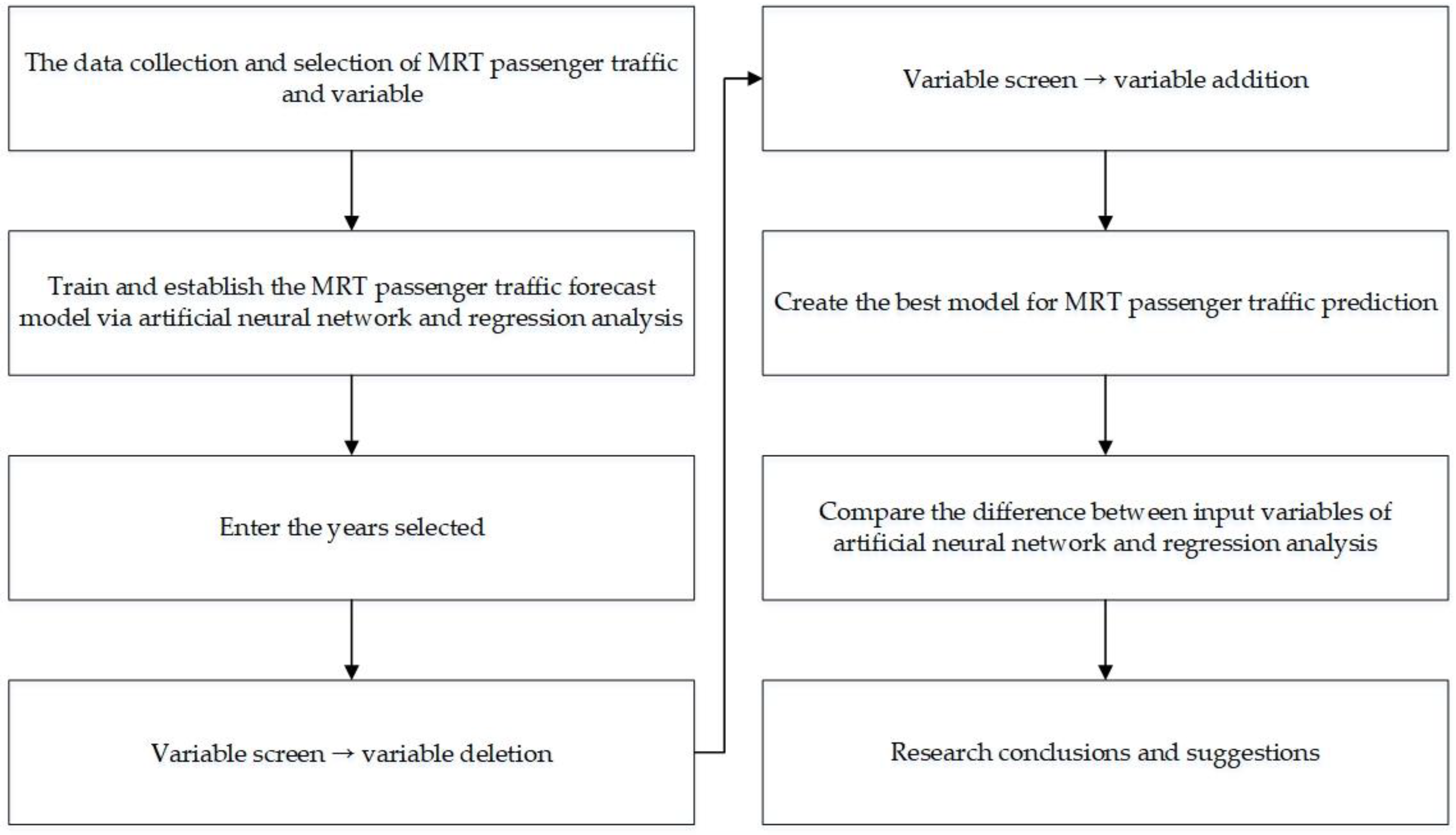
3.1. Research Structure

The flow of this study is shown in Figure 1, below, and the relevant steps are as follows:

• The literature and selected variables that may affect the MRT passenger traffic are collected via a literature review.
• The artificial neural network and regression analysis are adopted as research methods for training and establishing a prediction model of the MRT passenger traffic: (1) the years of training are selected; (2) the input variables of the MRT passenger traffic are deleted one by one, and the best variable is found; (3) the possible input variables that are likely to affect the MRT passenger traffic in the training are added, and the best variable is found; and (4) the MRT passenger traffic forecast model is established via an artificial neural network and regression analysis.
• The MRT passenger traffic forecast model is established.
• The advantages and disadvantages of the input variables selected are compared and analyzed, considering the results of the artificial neural network and regression analysis.
• The research conclusions and suggestions based on the research results are provided.

3.2. Research Design and Steps

We first collected the relevant literature and selected variables that could potentially affect the MRT passenger traffic via a literature review, as shown in Table 1, and then selected the years of training, as shown in

Table 3. Annual information of the variables in relation to passenger traffic.

Variable	X1	X2	X3	X4	...	X17	X18	X19	X20	Y1
Unit/Year	Million	Million	%	Km2 (Train)	...	Station	Km	Persons/Km	Persons (Thousand)	Total Persons
1996	8,146,092	8,036,590	6.18	500	...	12	10.5	57,226,810	102	11,174,359
1997	8,806,852	8,717,241	6.11	509	...	32	32.4	243,676,517	3282	31,081,395
1998	9,449,692	9,381,141	4.21	501	...	39	40.3	512,282,678	12,229	60,737,782
1999	9,906,113	9,815,595	6.72	495	...	56	56.4	1,031,342,472	21,203	126,952,122
2000	10,490,818	10,351,260	6.42	491	...	62	65.1	2,042,303,171	38,138	268,716,740
2001	10,350,233	10,158,209	−1.26	448	...	62	65.1	2,223,486,596	44,368	289,642,714
2002	10,923,385	10,680,883	5.57	437	...	62	65.1	2,469,037,312	53,093	324,433,557
2003	11,294,739	10,965,866	4.12	433	...	62	65.1	2,440,488,934	72,399	316,189,128
2004	12,021,744	11,649,645	6.51	428	...	63	67	2,680,355,529	125,350	350,141,956
2005	12,383,120	12,092,254	5.42	422	...	63	67	2,742,372,258	127,424	360,729,803
2006	12,952,502	12,640,803	5.62	415	...	69	74.4	3,002,988,957	130,916	384,003,220
2007	13,739,828	13,407,062	6.52	417	...	69	74.4	3,298,870,463	140,044	416,229,685
2008	13,465,596	13,150,950	0.70	418	...	70	75.8	3,513,969,060	152,643	450,024,415
2009	13,375,650	12,961,656	−1.57	428	...	82	90.6	3,720,991,244	153,679	462,472,351
2010	14,548,852	14,119,213	10.63	425	...	93	100.8	4,123,189,518	162,098	505,466,450
2011	14,700,572	14,312,200	3.80	425	...	94	101.9	4,607,801,411	170,963	566,404,489
2012	15,141,108	14,686,917	2.06	427	...	102	112.8	4,973,666,983	177,918	594,864,715
2013	15,646,211	15,221,201	2.23	428	...	109	121.3	5,234,160,050	182,193	634,961,083
2014	16,621,378	16,081,798	3.74	428	...	116	129.2	5,589,414,250	180,133	679,506,401
2015	17,485,375	16,881,614	3.78	429	...	117	131.1	5,880,980,257	173,877	717,511,809

.

The main structure of this study is established by the idea of an artificial neural network structure, including the input layer, hidden layer, and output layer. X1 to X10 are variables that may affect the Taipei MRT passenger traffic, while Y1 is the Taipei MRT passenger traffic. We first tested independent variables X1 to X10 and then carried out the deletion test, before adding independent variables X11 to X20 one by one. The purpose of this step was to screen the input variables with a lower correlation to the Taipei MRT passenger traffic to avoid interfering with the prediction results. The regression analysis is primarily used to discuss the causal result relationship among the variables and conduct the prediction via a line chart [20,21], a scatter chart [22], correlation analysis [23,24,25], the enter method [26,27], and stepwise regression [28,29,30].

3.2.1. Line Chart and Scatter Chart

The line chart demonstrates that the growth trend of the Taipei MRT passenger traffic (Figure 2) is relatively similar to the variable X1 GNP (Figure 3), and its effect is therefore assumed to be more important. From the scatter chart (Figure 4), if the variable X1 GNP and the Taipei MRT passenger traffic have a linear distribution, they should be more correlated, and the effect of variable X1 GNP on the Taipei MRT passenger traffic will be obvious.

3.2.2. Correlation Analysis

In correlation analysis, if two variables are significantly correlated, this only means that the strength and direction between the variables are significant. When the coefficient is significant, it only explains that the two variables are correlated at a certain level, including the strength and direction, instead of indicating the existence of a causal relationship. They may both be the cause and result at the same time, or a causal relationship may actually exist.

3.2.3. Enter Method

The enter method means that all the prediction variables must be entered into the regression formula, regardless of the significance of the individual variable.

3.2.4. Stepwise Regression

When variables are entered into the regression equation, the backward selection method is used to eliminate unimportant variables.

4. Empirical Analysis

This study uses regression analysis and class neural network methods to select and predict the variables affecting passenger traffic using the Taipei Metro passenger traffic trends from March 1996 to December 2015. Finally, we compare the results of the neural network and regression analysis prediction methods, evaluate and analyze the prediction performance of the two methods, and then select the best prediction model.

4.1. Regression Analysis

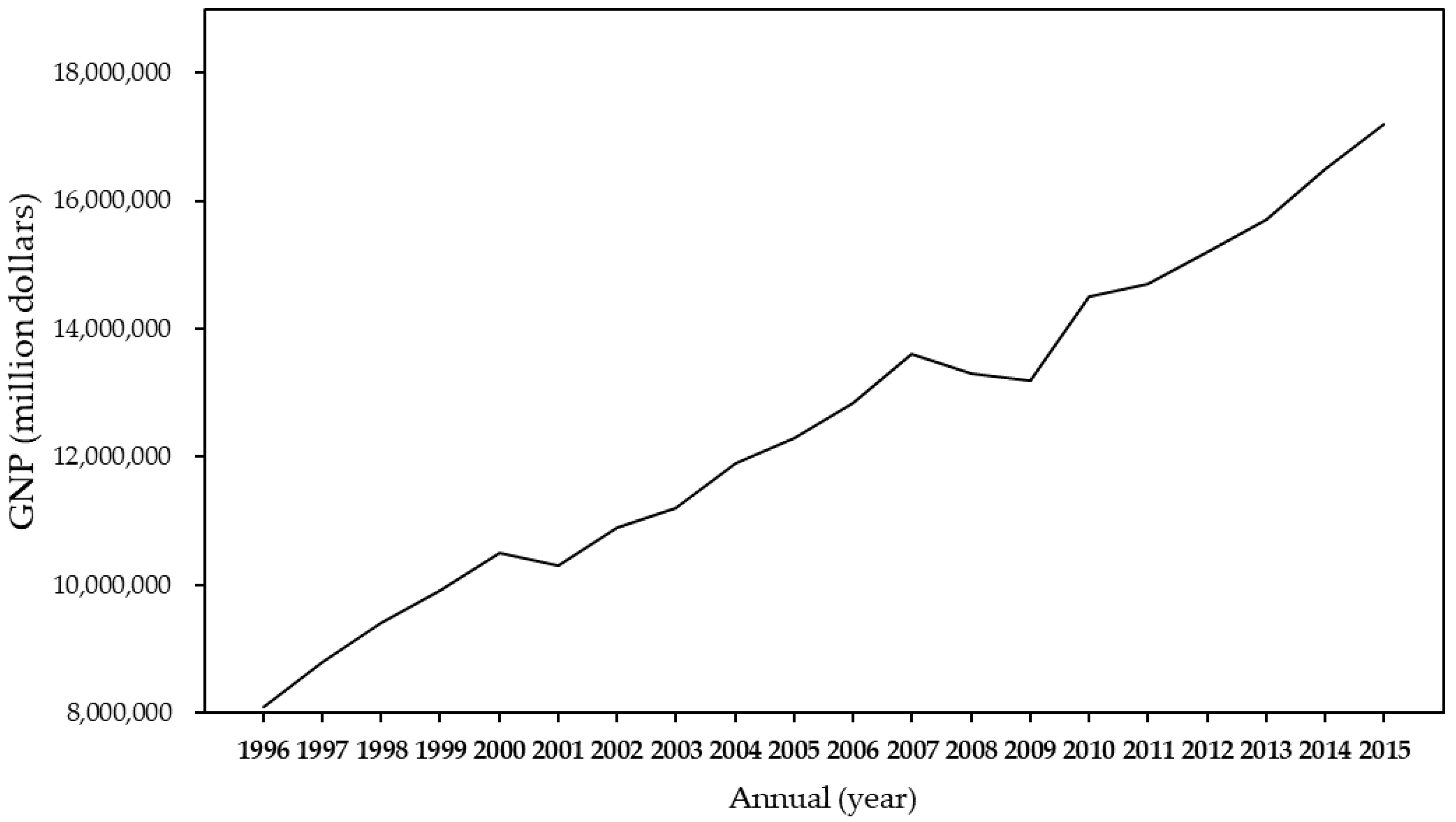
We adopted statistical software to analyze 20 parametric variables from March 1996 to December 2015 to explore the causal relationship between the variables as well as to make predictions through line graphs, scatter plots, correlation analysis, forced entry, and stepwise regression analysis to explore the causal relationship between the variables.

4.1.1. Line Chart

If the line graphs of the variables are found to be more similar to the growth trend line graphs of Taipei Metro’s passenger volume, it is speculated that the effect should be more important (Figure 5).

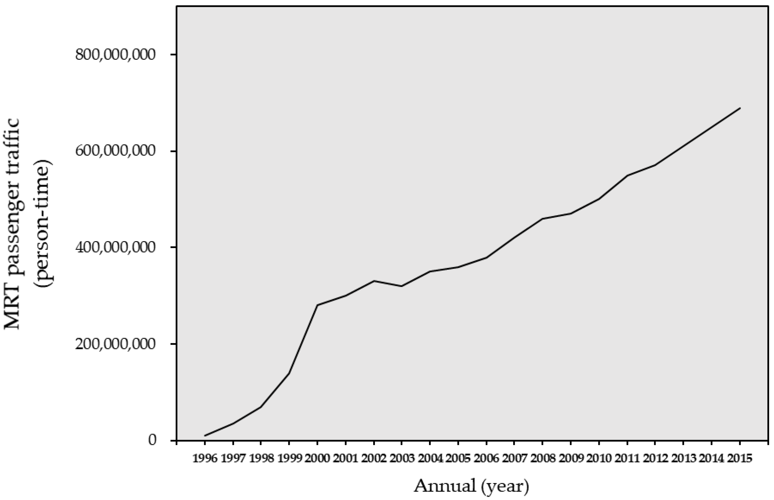
4.1.2. Scatter Chart

From the scatter plot, we can see that the correlation between the variables and Taipei Metro’s passenger volume is greater if they are clearly distributed in a straight line (Figure 6).

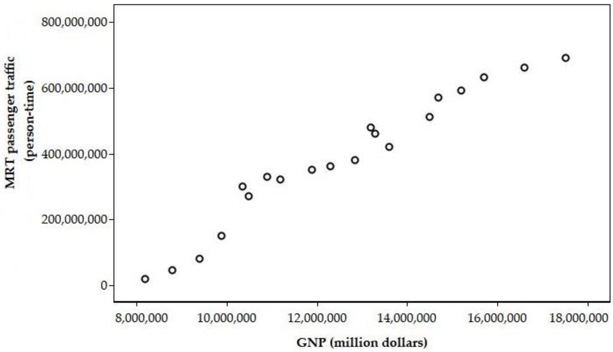
4.1.3. Correlation Analysis

The correlation coefficient primarily refers to the degree of correlation between the variables, while it does not verify the influence of the “independent variable” on the “dependent variable”. Therefore, the obtained correlation coefficient (R value) can only indicate that the two variables are positively correlated, negatively correlated, or independent. It cannot be interpreted as the effect of the independent variable on the dependent variable. In the interpretation of the correlation coefficient, positive and negative indicate the direction of the correlation, not the degree of the correlation. If the degree of the correlation is between the R values, i.e., between plus or minus 0.3 (i.e., between 0.3 and −0.3), it is considered a low correlation; it is considered a moderate correlation if the value is between plus or minus 0.3 to 0.6 (that is, between 0.3 and 0.6, or between −0.3 and −0.6); and if it is between plus or minus 0.6 to 0.9 (i.e., 0.6 to 0.9, or −0.6 to −0.9), it is considered a high correlation. If the R value is plus or minus 1, this indicates a complete correlation.

4.1.4. Entry Method

All the predictive variables are incorporated into the regression equation at the same time, and the least squares method and statistical software are used to calculate the complex regression model. The analysis of the explanatory variables is as follows.

Table 4. Forced entry method variables inputted/removed.

Model	Variable Inputted	Variable Removed	Method
1	X3, X4, X5, X6, X7, X8, X9, X10, X11, X12, X13, X14, X15, X16, X17, X20		Entry

, showing the entry variables inputted/removed, provides a list of variables that are subjected to regression analysis, including a total of 16 independent variables.

The variance analysis result of the forced entry method shows the overall verification of the model significance to verify the significance of the overall regression model. The quadratic sum of the regression model is 830,852,340,051,751,420, the total sum of squares is 830,902,477,461,923,070, the F value = 3107.157, and the p value = 0.000 < 0.05, which reaches significance. Furthermore, F is used to verify the regression model, F (α, K, N-K-1) = F(0.05, 16, 3) ≒ 8.7, and the F value of this regression equation = 3107.157 > critical value F value of 8.7, thus rejecting the null hypothesis and indicating that the explanatory power of the overall regression model reaches a significant level.

In

Table 5. Coefficients of the entry method.

				Collinearity Statistical Material
Model		T	Significance	Permissible Deviation	VIF
1	(Constant)	−2.374	0.098
	X1	0.685	0.543	0.094	10.601
	X3	2.787	0.069	0.004	263.957
	X4	1.500	0.231	0.002	457.889
	X5	1.429	0.248	0.001	1047.998
	X6	3.584	0.037	0.000	4167.205
	X8	−1.309	0.282	0.001	835.575
	X9	−3.509	0.039	0.001	1728.353
	X10	−1.115	0.346	0.007	143.916
	X11	2.919	0.062	0.005	206.473
	X12	1.151	0.333	0.007	142.958
	X13	−3.006	0.057	0.003	293.111
	X14	−1.913	0.152	0.003	313.741
	X15	0.030	0.978	0.002	617.120
	X16	11.990	0.001	0.003	374.019
	X17	−0.098	0.928	0.002	656.926
	X20	−2.325	0.103	0.003	348.165

, the coefficients of the forced entry method are the verification results of the multicollinearity of the output independent variables using statistical software. This model has a total of 16 independent variables and 17 eigenvalues, and the minimum tolerance is 0.000. If the tolerance is lower than 0.2, it is determined that there is collinearity between this independent variable and other independent variables. The highest VIF is 4167.205. In general, if the VIF is greater than 4, this means that the independent variable is collinear with other independent variables.

The variables excluded by the forced entry method demonstrate that there are four variables, including the total GNP, GDP, MRT mileage, and MRT extended passenger mileage, that did not enter the regression model. To reduce the collinearity problem of the multiple regression model, we adopted the stepwise method. The advantage of this method is that the variables are selected one by one according to the influence of the independent variable on the dependent variable, thus eliminating the collinearity problem.

4.1.5. Stepwise Method

To reduce the collinearity problem of multiple regression models, we adopted the stepwise method and performed calculations using statistical software. The following

Table 6. Stepwise regression variables inputted/removed.

Model	Variable Inputted	Method
1	X16	Step by step (criteria: F-to-enter probability ≤ 0.050, F-to-remove probability ≥ 0.100)
2	X20	Step by step (criteria: F-to-enter probability ≤ 0.050, F-to-remove probability ≥ 0.100)

was obtained.

Table 6 shows the stepwise regression variables inputted/removed and a list of stepwise method variables. The criteria for selection are: (F-to-enter probability ≤ 0.050, F-to-remove probability ≥ 0.100). In total, two variables are selected for the regression equation in two steps (models). In Model 1, MRT passenger revenue is selected. In Model 2, two-way transfer preferential volume is added. Therefore, the two variables of the MRT passenger revenue and two-way interchange preferential volume are selected for the model.

The analysis result of stepwise regression variance using Model 1 of the MRT passenger revenue variables shows that the F value of the overall regression model is 15,598.145, p = 0.000 < 0.05, reaching significance and indicating a significant correlation between the independent variable (the MRT passenger revenue) and the dependent variable (the Taipei MRT passenger traffic). Taking Model 2 as an example, the F value of the regression model of Model 2 is 12,741.962, p = 0.000 < 0.05, which reaches significance and indicates a significant correlation between the independent variable (the preferential volume of two-way interchange) and the dependent variable (the Taipei MRT passenger traffic). The two variables can effectively predict the passenger traffic of the Taipei MRT.

Table 7. Stepwise regression coefficients.

Model		Unstandardized Coefficients		Standardized Coefficients	T	Significance
		B	Standard Error	Beta
1	(Constant)	−12,082,965.667	3,520,486		−3.432	0.003
	X16	0.047	0	0.999	124.893	0
2	(Constant)	−9,989,402.575	2,818,390		−3.544	0.002
	X16	0.044	0.001	0.942	53.482	0
	X20	193.099	54.85	0.062	3.52	0.003

demonstrates a positive relationship between the MRT passenger revenue and the preferential volume of the two-way passenger transfer—two independent variables in the table of stepwise regression coefficients, both of which were consistent with the prediction and significant.

Table 8. Variables excluded by the stepwise method.

Model		Beta	T	Significance	Partial Correlation
1	X1	0.031	0.799	0.436	0.190
	X2	0.024	0.641	0.530	0.154
	X3	0.007	0.780	0.446	0.186
	X4	−0.031	−2.705	0.015	−0.549
	X5	−0.020	−1.234	0.234	−0.287
	X6	0.100	2.949	0.009	0.582
	X7	0.085	2.668	0.016	0.543
	X8	0.009	0.371	0.715	0.090
	X9	0.080	1.411	0.176	0.324
	X10	0.002	0.071	0.944	0.017
	X11	0.025	1.981	0.064	0.433
	X12	0.016	0.782	0.445	0.186
	X13	−0.008	−0.204	0.841	−0.049
	X14	0.012	0.481	0.637	0.116
	X15	−0.039	−0.831	0.418	−0.197
	X17	−0.058	−1.788	0.092	−0.398
	X18	−0.063	−1.873	0.078	−0.414
	X19	0.220	1.473	0.159	0.336
	X20	0.062	3.520	0.003	0.649
2	X1	−0.026	−0.750	0.464	−0.184
	X2	−0.030	−0.900	0.382	−0.219
	X3	0.004	0.562	0.582	0.139
	X4	−0.015	−1.232	0.236	−0.294
	X5	−0.007	−0.519	0.611	−0.129
	X6	0.050	1.239	0.233	0.296
	X7	0.021	0.471	0.644	0.117
	X8	−0.017	−0.804	0.433	−0.197
	X9	−0.076	−1.158	0.264	−0.278
	X10	−0.018	−0.708	0.489	−0.174
	X11	−0.007	−0.447	0.661	−0.111
	X12	−0.026	−1.306	0.210	−0.310
	X13	−0.032	−1.015	0.325	−0.246
	X14	−0.011	−0.519	0.611	−0.129
	X15	−0.024	−0.637	0.533	−0.157
	X17	−0.027	−0.945	0.359	−0.230
	X18	−0.033	−1.093	0.290	−0.264
	X19	0.090	0.698	0.495	0.172

demonstrates the stepwise mode analysis results of the variable table excluded by stepwise regression, with two variables remaining: the MRT passenger revenue and two-way interchange preferential volume. From Table 8, it can also be understood that the variables may enter the regression model because the correlation value of the dependent variables is the highest in Model 1, where the preferential volume of two-way interchange is 0.649. In Model 2, the correlation value of the total amount of goods imported into Taiwan is −0.310, which is the highest.

We used statistical software to analyze the inputting of 20 parameter variables from 1996 to 2013 and outputting of the predictive value of the passenger traffic of the Taipei MRT (

Table 9. Predictive value of regression analysis.

Year of Observation	Actual Number of MRT Passengers	Predictive Value of Regression Analysis	Residual Value
1996	11,174,359	3,305,117	7,869,242
1997	31,081,395	36,987,970	−5,906,575
1998	60,737,782	68,054,760	−7,316,978
1999	126,952,122	129,264,711	−2,312,589
2000	268,716,740	270,052,789	−1,336,049
2001	289,642,714	287,079,395	2,563,319
2002	324,433,557	319,060,611	5,372,946
2003	316,189,128	312,874,254	3,314,874
2004	350,141,956	351,632,592	−1,490,636
2005	360,729,803	359,697,272	1,032,531
2006	384,003,220	385,978,346	−1,975,126
2007	416,229,685	421,166,927	−4,937,242
2008	450,024,415	449,687,066	337,349
2009	462,472,351	457,533,201	4,939,150
2010	505,466,450	495,603,126	9,863,324
2011	566,404,489	560,822,898	5,581,591
2012	594,864,715	607,214,292	−12,349,577
2013	634,961,083	638,210,638	−3,249,555

). The predicted value was calculated according to the predicted value table of the progressive regression analysis using the MAPE formula. The result obtained using the regression analysis prediction method was MAPE = 6.47%.

4.2. Artificial Neural Network

Using the training data from 1996 to 2013 as the artificial neural network training materials and those from 2014 to 2015 as the sample data, we were able to use a total of 20 parameters as the input variables of the artificial neural network; the output variables were the passenger traffic prediction values of the Taipei MRT. Statistical software was used to analyze 20 parametric variables from 1996 to 2015, before the input variables were converted into an artificial neural network to investigate the causal relationship between the variables and make predictions based on a line chart, scatter chart, correlation analysis, forced entry method, and stepwise method. Therefore, the artificial neural network does not temporarily delete any variables and inputs all of them into the artificial neural network. Then, the optimal combination of input variables was analyzed.

4.2.1. Year of Selection

Basic information on the year of selection for variables X1 to X20 and the output variable Y1 is shown in Table 3, where Y1 stands for the Taipei MRT passenger traffic. Using the backward propagation artificial neural network algorithm model, the average absolute percentile error was used to analyze 7 years/2 years of training, 6 years/2 years of training, and 5 years/2 years of training from 1996 to 2015, and the training results are shown in

Table 10. Year selection of the artificial neural network.

Evaluation Indicators	7 Years/2 Years of Training (1996–2002/2003–2004)	6 Years/2 Years of Training (2003–2008/2009–2010)	5 Years/2 Years of Training (2009–2013/2014–2015)
MAPE	8.26%	4.35%	2.45%

. This study uses the training model of 5 years/2 years of training prediction for empirical research.

4.2.2. Deleted Variables

First, we used the 5-year and 2-year training modes (2009 to 2013 and 2014 to 2015) and then deleted the X1 to X10 variables in order, selecting the variables with the highest MAPE value for deletion. The purpose of this was to screen out variables that have little influence on the passenger traffic of the Taipei MRT to avoid interference with the predicted results. After the deletion was complete, we then started the training process to determine the best variables and improve the accuracy of the prediction results.

4.2.3. The Output Results of the Artificial Neural Network

Using the training data from 1996 to 2013 as the artificial neural network training materials and the data from 2014 to 2015 as the sample data, we used a total of 20 parameters as the input variables of the artificial neural network; the output variables were the passenger traffic prediction values of the Taipei MRT (

Table 11. Predictive values of the artificial neural network.

Year of Observation	Actual Number of MRT Passengers	Predictive Values of the Artificial Neural Network	Residual Value
1996	11,174,359	15,320,813	4,146,454
1997	31,081,395	30,226,981	−854,414
1998	60,737,782	60,188,236	−549,546
1999	126,952,122	126,305,437	−646,685
2000	268,716,740	267,922,813	−793,927
2001	289,642,714	289,012,656	−630,058
2002	324,433,557	324,181,085	−252,472
2003	316,189,128	327,612,737	11,423,609
2004	350,141,956	349,893,508	−248,448
2005	360,729,803	360,534,282	−195,521
2006	384,003,220	383,858,990	−144,230
2007	416,229,685	415,952,914	−276,771
2008	450,024,415	285,870,926	−164,153,489
2009	462,472,351	462,125,697	−346,654
2010	505,466,450	505,270,408	−196,042
2011	566,404,489	565,977,673	−426,816
2012	594,864,715	616,442,418	21,577,703
2013	634,961,083	630,207,775	−4,753,308

).

According to the prediction values, shown in Table 10, of the artificial neural network, calculated by the MAPE formula, the result obtained by the neural network prediction method is MAPE = 4.82%. To compare the predicted values of regression analysis with those of the artificial neural network, the results showed that the MAPE value of the regression analysis was 6.47%. The MAPE value of the artificial neural network was 4.82%, so the artificial neural network has the best prediction outcomes.

4.3. Comparison of Regression Analysis and Artificial Neural Networks

4.3.1. Deletion of the Forced Entry Method of Regression Analysis to Exclude Four Variables

Using the 5-year training for 2 years (2009–2013/2014–2015) model, we deleted the four eliminated variables of the regression analysis, which were the GNP, GDP, MRT mileage, and MRT extended passenger mileage. Using a total of 16 parameters as the input variables for the regression analysis and artificial neural network comparison, it was found that the MAPE value predicted by regression analysis was 0.94%, and the MAPE value of the artificial neural network was 0.54%. Both methods showed the best prediction results.

4.3.2. Deletion of Four Variables with High MAPE Values in Artificial Neural Networks

Using the model of 5-year training for 2 years (2009–2013/2014–2015), we deleted the four variables with the highest MAPE values in the artificial neural network, which included the economic growth rate, personal income, total amount of goods imported into Taiwan, and number of MRT stations. In total, 16 parameters were used as the input variables for the regression analysis and artificial neural network comparison, and it was found that the MAPE value predicted by regression analysis was 0.62%. The MAPE value of the artificial neural network was 0.31%. Both methods showed the best prediction results.

4.3.3. Collinearity Verification

In order to verify whether the independent variable of the MRT passenger revenue is collinear with the dependent variable of the MRT passenger traffic, statistical software was used to analyze the inputting of 19 parameter variables from 1996 to 2013 and outputting of the passenger traffic prediction value of the Taipei MRT. Again, the training data from 1996 to 2013 were used as the artificial neural network training materials, and the data from 2014 to 2015 were used as the sample data. In total, 19 parameters were used as the input variables of the artificial neural network, while the output variable was the passenger traffic prediction value of the Taipei MRT. Twenty variables and 19 parameter variables were used to compare the predictive values of the regression analysis and artificial neural network after removing the independent variable, the MRT revenue. The results showed that the MAPE residual value of the regression analysis was 1.28%, and the MAPE residual value of the artificial neural network was 0.19%. We observed no significant difference between the two, which proves that there was no collinearity problem after deleting the independent variable, the MRT passenger revenue.

4.3.4. Monthly Passenger Traffic Experiment

In this study, we collected data on passenger traffic (month) and related variables (month); however, because some data were recorded at different times, 167 regression analyses were conducted from January 2000 to December 2015 (excluding the incomplete data on Cyclone Nari in September 2001). The neural network used the mode of 2000–2013 training 2014–2015 and the following seven parameter variables: the MRT operation mileage, MRT station number, MRT train number, MRT extended vehicle mileage, MRT extended passenger mileage, MRT passenger revenue, and two-way transit preferential volume. The output variable is the passenger traffic prediction value of the Taipei MRT. The results showed that the MAPE value of the regression analysis was 1.45%, and the MAPE value of the artificial neural network was 0.42%. Both methods showed the best prediction results.

4.4. Summary of the Empirical Results

The results of this study are shown in

Table 12. Summary of the empirical results of the regression analysis and artificial neural network.

Experiment Module	Regression Analysis MAPE Value	Artificial Neural Network MAPE Value	Results
20 variables	6.47%	4.82%	The artificial neural network is better.
The four variables excluded in the regression analysis were deleted: the GNP, GDP, MRT mileage, and MRT extended passenger mileage.	0.94%	0.54%	Both had the best prediction results.
The four variables with the highest MAPE values were deleted: the economic growth rate, personal income, total amount of goods imported into Taiwan, and number of MRT stations.	0.62%	0.31%	Both had the best prediction results.
19-variable collinearity verification (deletion of the MRT passenger revenue).	5.19%	4.63%	There is no collinearity problem.
Monthly passenger traffic experiment.	1.45%	0.42%	Both had the best prediction results.

, which summarizes the empirical results of the regression analysis and artificial neural network.

5. Analysis of Empirical Results

The results and research contributions of this paper in relation to passenger traffic prediction provide a valuable reference for both academics and practitioners. They are summarized in this section.

5.1. Analysis of Results

In this study, we used an artificial neural network and regression analysis to construct the Taipei MRT passenger traffic prediction model. Seven findings of this study are worth summarizing:

• A total of 20 parameters from 1996 to 2013 were used as the input variables of the regression analysis, and the output value was the passenger traffic prediction value of the Taipei MRT. The stepwise regression of the regression analysis, predicting the MAPE value of the Taipei MRT passenger traffic, is 6.47%, which demonstrates an excellent predictive performance.
• Using the training data from 1996 to 2015 as artificial neural network training materials and the data from 2013 to 2015 as the sample data, a total of 20 parameters were used as the input variables of the artificial neural network; the output value was the passenger traffic prediction value of the Taipei MRT. Using an artificial neural network to predict the MAPE value of the Taipei MRT passenger traffic, the result was 4.82%, which demonstrates an excellent predictive performance.
• We used the 5-year training for 2 years (2009–2013/2014–2015) model and deleted the already eliminated four variables of regression analysis, which were the GNP, GDP, MRT mileage, and MRT extended passenger mileage. In total, 16 parameters were used as the input variables for regression analysis and artificial neural network comparison. The MAPE value predicted by regression analysis was found to be 0.94%, and the MAPE value of the artificial neural network was 0.54%. Both methods had the best prediction results.
• We used the model of 5-year training for 2 years (2009–2013/2014–2015) and deleted the four variables with the highest MAPE values in the artificial neural network, including the economic growth rate, personal income, total amount of goods imported into Taiwan, and number of MRT stations. In total, 16 parameters were used as the input variables for regression analysis and artificial neural network comparison. The MAPE value predicted by regression analysis was 0.62%, and the MAPE value of artificial neural networks was 0.31%. Both methods had the best prediction results.
• In order to verify whether the independent variable MRT passenger revenue is collinear with the dependent variable MRT passenger traffic, we applied statistical software to analyze the inputting of 19 parameter variables from 1996 to 2013 and outputting of the passenger traffic prediction value of the Taipei MRT. Again, we used the training data from 1996 to 2015 as the artificial neural network training materials and the data from 2013 to 2015 as the sample data. We used a total of 19 parameters as the input variables of the artificial neural network and the passenger traffic prediction value of the Taipei MRT as the output value in order to compare the predictive values of the regression analysis and artificial neural network. The result showed that the MAPE value of the regression analysis was 5.19%, and the MAPE value of the artificial neural network was 4.63%. Twenty variables and 19 parameter variables were used to compare the predictive values of the regression analysis and artificial neural network after removing the independent variable, the MRT revenue. The results showed that the MAPE residual value of regression analysis was 1.28%, and the MAPE residual value of the artificial neural network was 0.19%. No significant difference was observed between them, which proves that there is no collinearity problem after deleting the independent variable, the MRT passenger revenue.
• We collected data on the passenger traffic (month) and related variables (month); however, because some data were recorded at different times, 167 regression analyses were conducted from January 2000 to December 2015 (excluding the incomplete data on Cyclone Nari in September 2001). The neural network used the mode of 2000–2013 training 2014–2015 and the following seven parameter variables: the MRT operation mileage, MRT station number, MRT train number, MRT extended vehicle mileage, MRT extended passenger mileage, MRT passenger revenue, and two-way transit preferential volume. The output value is the passenger traffic prediction value of the Taipei MRT. The results show that the MAPE value of regression analysis was 1.45%, and the MAPE value of the artificial neural network was 0.42%. Both methods had the best prediction results.
• This study investigated the passenger traffic prediction of the Taipei MRT and analyzed and constructed the prediction model based on two prediction methods: regression analysis and artificial neural networks. The results are presented to allow transportation organizations to maximize their profits by making plans and decisions relating to future operations based on past passenger traffic trends.

5.2. Research Contributions

To improve the utilization rate of the metro area’s transportation system and reduce environmental pollution by combining it with the public transportation system of the MRT station, the following research contributions are provided:

1.

Choosing the right forecasting tools for business planning and decision making.

The amount of passenger traffic significantly impacts the transportation industry, and accurate prediction depends on a full understanding of the metropolitan environment and analysis of the factors that influence demand. The commonly used methods for forecasting passenger traffic demand include statistical regression analysis, econometric modeling, time-series modeling, neural-network modeling, gray theory, etc.; selecting the appropriate forecasting tools can allow for the maximization of profits by aiding in planning and decision making relating to future operations based on past passenger traffic trends.

2.

Construction and planning of transport systems.

Passenger traffic prediction is a very important factor in the construction and planning of transportation systems and serves as the essential basis for putting forward requirements for the construction and expansion of transportation equipment. Therefore, the results of this study can be used as a reference for transportation organizations, such as operation management, manpower allocation, shift distance, transportation demand, etc.

3.

Curbing the growth of private vehicles.

The excessively increased use of private vehicles will cause such problems as air pollution, noise, road congestion, traffic accidents, etc., and the social costs shall be shared by the public. Therefore, strengthening the control on the increase of private vehicles is necessary, and passenger traffic prediction cooperates perfectly with public transportation transfer system construction, encouraging people to transfer from private vehicles to public transport systems and then improving ridership on public transportation systems.

4.

Public transportation leads to urban development.

With the public transport system as the backbone of urban development, passenger traffic prediction can establish a different planning method and procedure from traditional urban development, implement the priority concept of public transportation, look toward the future, and actively promote subsequent MRT-related construction based on the existing construction. In addition to being safe and convenient, public transportation systems can also inhibit the growth of private transportation, reduce carbon while promoting energy saving, and build low-carbon and green energy cities.

5.

Improvement of the efficiency of all public transport vehicles.

In this study, the data on MRT passenger traffic prediction not only provide traffic dispatching and transport strategic planning data but also combine them with the electronic ticket or passenger traffic data of public transport vehicles, such as the high-speed railways, Taiwan’s railways, urban buses, and UBikes around the MRT stations, to conduct the overall passenger traffic analysis. This is used as the basis for the planning and operation management of the public transport system to improve the efficiency and service quality of each public transport vehicle and thus maximize the benefit of passenger traffic prediction.

6. Conclusions

This study investigated the passenger traffic prediction of the Taipei MRT and analyzed and constructed the prediction model based on two prediction methods: regression analysis and artificial neural networks. The results are presented as a reference for transportation organizations to allow them to maximize profits by making plans and decisions relating to future operations based on past passenger traffic trends.

During this research, we discussed with senior executives of MRT companies and found that accurate passenger traffic prediction can effectively reduce costs. The management implications of this study are as follows:

• The forecasting of passenger traffic has a great influence on the transportation industry, and transportation organizations can make plans and decisions for future operations based on past passenger traffic trends. Therefore, it is very important for transportation organizations to have a clear and objective forecasting method.
• Based on past research data and a literature review, we determined the variable that affects the forecasting of passenger traffic demand the most. The forecasting of the MRT passenger traffic affects the future economic development of Taipei City and New Taipei City, so it is necessary to select the appropriate passenger traffic forecasting tool.
• The data on passenger traffic forecasting in this study not only allow for the planning of traffic dispatching, operation management, manpower allocation, shift distance, transportation demand, etc., but also serve as an essential basis for transportation organizations, enabling them to put forward requirements for the construction and expansion of transportation equipment.

Despite the limitations of this study, we believe that the findings and management implications of our study are intriguing enough to invite future research on the topic of passenger traffic forecasting, as well as future research on other traffic-related topics.

References

1. Verbavatz, V.; Barthelemy, M. Access to mass rapid transit in OECD urban areas. Sci. Data 2020, 7, 1–6. [Google Scholar] [CrossRef]
2. Wiseman, Y. Autonomous vehicles. In Encyclopedia of Information Science and Technology, 5th ed.; IGI Global: Hershey, PA, USA, 2021; pp. 1–11. [Google Scholar]
3. Wiseman, Y. Driverless cars will make passenger rail obsolete [Opinion]. IEEE Technol. Soc. Mag. 2019, 38, 22–27. [Google Scholar] [CrossRef]
4. Yang, Z.; Li, C.; Jiao, J.; Liu, W.; Zhang, F. On the joint impact of high-speed rail and megalopolis policy on regional economic growth in China. Transp. Policy 2020, 99, 20–30. [Google Scholar] [CrossRef]
5. Lio, W.; Liu, B. Uncertain maximum likelihood estimation with application to uncertain regression analysis. Soft Comput. 2020, 24, 9351–9360. [Google Scholar] [CrossRef]
6. Toraman, S.; Alakus, T.B.; Turkoglu, I. Convolutional capsnet: A novel artificial neural network approach to detect COVID-19 disease from X-ray images using capsule networks. Chaos Solitons Fractals 2020, 140, 110122. [Google Scholar] [CrossRef]
7. Mazanec, J.A. Classifying tourists into market segments: A neural network approach. J. Travel Tour. Mark. 1992, 1, 39–60. [Google Scholar] [CrossRef]
8. Law, R.; Au, N. A neural network model to forecast Japanese demand for travel to Hong Kong. Tour. Manag. 1999, 20, 89–97. [Google Scholar] [CrossRef]
9. Kulendran, N.; Witt, S.F. Leading indicator tourism forecasts. Tour. Manag. 2003, 24, 503–510. [Google Scholar] [CrossRef]
10. Grosche, T.; Rothlauf, F.; Heinzl, A. Gravity models for airline passenger volume estimation. J. Air Transp. Manag. 2007, 13, 175–183. [Google Scholar] [CrossRef]
11. Shams, S.R.; Jahani, A.; Moeinaddini, M.; Khorasani, N. Air carbon monoxide forecasting using an artificial neural network in comparison with multiple regression. Model. Earth Syst. Environ. 2020, 6, 1467–1475. [Google Scholar] [CrossRef]
12. Liu, S.; Mocanu, D.C.; Matavalam, A.R.R.; Pei, Y.; Pechenizkiy, M. Sparse evolutionary deep learning with over one million artificial neurons on commodity hardware. Neural Comput. Appl. 2020, 1–16. [Google Scholar] [CrossRef]
13. Sun, W.; Huang, C. A carbon price prediction model based on secondary decomposition algorithm and optimized back propagation neural network. J. Clean. Prod. 2020, 243, 118671. [Google Scholar] [CrossRef]
14. Liu, R.; Mancuso, C.A.; Yannakopoulos, A.; Johnson, K.A.; Krishnan, A. Supervised learning is an accurate method for network-based gene classification. Bioinformatics 2020, 36, 3457–3465. [Google Scholar] [CrossRef] [PubMed]
15. Shirokanev, A.S.; Kirsh, D.V.; Kupriyanov, A.V. Research of an algorithm for crystal lattice parameter identification based on the gradient steepest descent method. Comput. Opt. 2017, 41, 453–460. [Google Scholar] [CrossRef]
16. Hemilä, H.; Chalker, E. Vitamin C may reduce the duration of mechanical ventilation in critically ill patients: A meta-regression analysis. J. Intensive Care 2020, 8, 15. [Google Scholar] [CrossRef] [Green Version]
17. Şahin, U.; Şahin, T. Forecasting the cumulative number of confirmed cases of COVID-19 in Italy, UK and USA using fractional nonlinear grey Bernoulli model. Chaos Solitons Fractals 2020, 138, 109948. [Google Scholar] [CrossRef]
18. Prado, F.; Minutolo, M.C.; Kristjanpoller, W. Forecasting based on an ensemble autoregressive moving average-adaptive neuro-fuzzy inference system–neural network-genetic algorithm framework. Energy 2020, 197, 117159. [Google Scholar] [CrossRef]
19. Longo, G.A.; Righetti, G.; Zilio, C.; Ortombina, L.; Zigliotto, M.; Brown, J.S. Application of an Artificial Neural Network (ANN) for predicting low-GWP refrigerant condensation heat transfer inside herringbone-type Brazed Plate Heat Exchangers (BPHE). Int. J. Heat Mass Transf. 2020, 156, 119824. [Google Scholar] [CrossRef]
20. Feng, Y.; Yang, T.; Niu, Y. Subpixel computer vision detection based on wavelet transform. IEEE Access 2020, 8, 88273–88281. [Google Scholar] [CrossRef]
21. Sohn, C.; Choi, H.; Kim, K.; Park, J.; Noh, J. Line Chart understanding with convolutional neural network. Electronics 2021, 10, 749. [Google Scholar] [CrossRef]
22. Shibzukhov, Z.M. Robust method for finding the center and the scatter matrix of the cluster. J. Phys. Conf. Ser. 2020, 1479, 012045. [Google Scholar] [CrossRef]
23. Peng, Q.; Wen, F.; Gong, X. Time-dependent intrinsic correlation analysis of crude oil and the US dollar based on CEEMDAN. Int. J. Financ. Econ. 2021, 26, 834–848. [Google Scholar] [CrossRef]
24. Shi, J.; Liu, B.; Qin, J.; Jiang, J.; Wu, X.; Tan, J. Experimental study of performance of repair mortar: Evaluation of in-situ tests and correlation analysis. J. Build. Eng. 2020, 31, 101325. [Google Scholar] [CrossRef]
25. Ibrahim, M.S.; Sidiropoulos, N.D. Reliable detection of unknown cell-edge users via canonical correlation analysis. IEEE Trans. Wirel. Commun. 2020, 19, 4170–4182. [Google Scholar] [CrossRef]
26. Di Tella, M.; Romeo, A.; Benfante, A.; Castelli, L. Mental health of healthcare workers during the COVID-19 pandemic in Italy. J. Eval. Clin. Pract. 2020, 26, 1583–1587. [Google Scholar] [CrossRef]
27. Moskowitz, S.; Dewaele, J.M. Is teacher happiness contagious? A study of the link between perceptions of language teacher happiness and student attitudes. Innov. Lang. Learn. Teach. 2021, 15, 117–130. [Google Scholar] [CrossRef]
28. Liu, B.; Zhao, Q.; Jin, Y.; Shen, J.; Li, C. Application of combined model of stepwise regression analysis and artificial neural network in data calibration of miniature air quality detector. Sci. Rep. 2021, 11, 1–12. [Google Scholar]
29. Hornby, T.G.; Henderson, C.E.; Holleran, C.L.; Lovell, L.; Roth, E.J.; Jang, J.H. Stepwise regression and latent profile analyses of locomotor outcomes poststroke. Stroke 2020, 51, 3074–3082. [Google Scholar] [CrossRef]
30. Żogała-Siudem, B.; Jaroszewicz, S. Fast stepwise regression based on multidimensional indexes. Inf. Sci. 2021, 549, 288–309. [Google Scholar] [CrossRef]
Figure 1. Research structure.
Electronics 10 01048 g001
Figure 2. The line chart of the total Taipei MRT passenger traffic.
Electronics 10 01048 g002
Figure 3. The line chart of the annual GNP.
Electronics 10 01048 g003
Figure 4. The scatter chart of the MRT passenger traffic and GNP.
Electronics 10 01048 g004
Figure 5. Line chart of the MRT passenger traffic.
Electronics 10 01048 g005
Figure 6. Scatter chart of GNP and MRT passenger traffic.
Electronics 10 01048 g006