A Neural Network Classifier with Multi-Valued Neurons for Analog Circuit Fault Diagnosis

Abstract

In this paper, we present a new method designed to recognize single parametric faults in analog circuits. The technique follows a rigorous approach constituted by three sequential steps: calculating the testability and extracting the ambiguity groups of the circuit under test (CUT); localizing the failure and putting it in the correct fault class (FC) via multi-frequency measurements or simulations; and (optional) estimating the value of the faulty component. The fabrication tolerances of the healthy components are taken into account in every step of the procedure. The work combines machine learning techniques, used for classification and approximation, with testability analysis procedures for analog circuits.

1. Introduction

The fault diagnosis problem of analog circuits can be considered to be far from a definitive solution, even if in the last years a large amount of research has been dedicated to it (e.g., [1,2,3,4,5,6,7,8,9,10,11,12]). This is because the growing complexity of electronic circuits and the increasing number of applications characterized by the coexistence of digital and analog systems. In fact, for analog circuits, the difficulty of using a univocal fault model, the presence of fault tolerances, noise effects, the large variability of input-to-output relationships, the limited accessibility of test points, and the presence of nonlinearities make fault diagnosis automation and fault location procedures very complex. As a consequence, the automation of fault diagnosis for analog circuits is significantly less advanced than for the digital case, for which fully automated testing methodologies have been developed and are commonly used.

A recent survey on fault diagnosis has summarized many methods proposed in the last few years, highlighting how much work still has to be done [13]. Roughly speaking, the analog fault diagnosis problem can be addressed via two main approaches: simulation-before-test (SBT) and simulation-after-test (SAT). The simulation of different possible faults and the collection of results in a dedicated dictionary are required for SBT approaches. The circuit responses are then compared with the dictionary for locating the faults. This approach is usually suitable for single catastrophic faults, because the size of the dictionary becomes very large in case of multiple parametric fault situations. In the SAT approach, instead, looking at the responses of the faulty network to a test stimulus, all element values can be identified by comparing the circuit responses with the network function equations. This approach is suitable for diagnosing parametric faults, i.e., deviations of parameter values from their tolerance range.

A lot of different techniques are used for analog fault diagnosis and, among them, those based on neural networks (NNs) exploit a mechanism for adaptive pattern classification. Unlike model-based techniques, neural networks allow for a robust classification, even in the case of poorly defined models and noisy environments. Given their data-driven nature, neural network-based failure diagnosis methods could be classified as an SBT technique. However, the great generalization capability of neural networks makes comparison between measurements and a fault dictionary unnecessary. After the training phase, the classifier structure contains all of the information necessary to process unknown data. Furthermore, the need to apply an algorithm evaluating the network output as a function of inputs and weight values allows us to see the method as a SAT approach.

One of the first approaches for the neural network-based analog fault diagnosis was proposed by Spina and Upadhyaya [14]. They used a feedforward neural network with the error backpropagation learning algorithm. Features extracted from the circuit response to a white noise were applied to its input. The neural network approach was improved by M. Aminian and F. Aminian via data preprocessing techniques such as wavelet decomposition and principal component analysis [15,16,17]. However, these approaches have strong limitations due to the lack of a testability analysis of the problem, which is an important prerequisite to a successful fault diagnosis strategy, as recently remarked [18,19,20]. By identifying how many and which components is possible to diagnose in the event of a failure, the testability analysis also allows the definition of the maximum diagnostic performance. In fact, the testability index represents an a priori evaluation of the solvability level of the problem and allows for the identification of ambiguities that make it impossible to detect the fault.

In the case of neural network-based fault diagnosis approaches, there is a particular aspect of testability analysis that needs to be carefully considered. In fact, testability analysis allows for the determination of a set of components representative of all the circuit elements [21]. In this way it is possible to confine the presence of faults to well-defined groups of components called fault classes (FCs). This information is very important in the case of fault diagnosis procedures based on the use of neural networks, because it drives the building of the network architecture. In fact, the network outputs must correspond to the FCs so that network training is performed to identify distinguishable faults. In ref. [22], an approach based on testability analysis for building the network architecture presents an improved behavior with respect to [14,15,16,17], so demonstrating the importance of the information given by this kind of analysis. Further examples of the strategic role of testability analysis are the recently proposed analog fault diagnosis methods under the single-input single-output single-fault scenario [8,9]. They are indeed quite interesting because they do not require the knowledge of the analytic expression of the network functions and are, in turn, predicated on a fault model in the form of a geometric locus in the complex plane. On the other hand, a not completely rigorous application of testability analysis results in some mistakes and conceptual discrepancies [23].

In recent years, support vector machines (SVM) have often been successfully used in place of neural networks for the fault diagnosis of analog circuits [24,25,26] by exploiting the great classifier capability of this kind of machine learning approach. Another recent category of machine learning approaches includes deep-learning NN [27].

More recently, a new generation of a multi-valued neuron-based multilayer neural network (MLMVN) with complex-valued inputs, weights, and outputs has demonstrated to have great classification capability [28,29,30,31]. We used it in this work to compare the results with those obtained using SVM.

The overall aim of this paper was to show how an accurate testability analysis, the use of a MLMVN neural network, sensitivity analysis, and a suitable choice of the test frequencies could be synergically employed to implement an efficient fault diagnosis method for analog circuits under the single-fault hypothesis. Sensitivity analysis helps identify which parameters produce stronger effects on the output as a consequence of their variations, while a suitable choice of the test frequencies helps minimizing the effect of measurement errors and component tolerances [32,33]. Finally, the possibility to vary the faulty parameters over a large range is an important characteristic not present in the most part of fault diagnosis literature.

It should also be taken into account that the “single fault” hypothesis adopted in this work was not only relevant in the analytical development of the proposed method, but was definitely the most interesting in the family of applications considered in this paper. On the other hand, the followed approach did not prevent us from extending the procedure to the multiple fault case.

The paper is structured as follows. Section 2 briefly describes the main tools used to perform the requested operations. Section 3 provides the theoretical background to the testability and ambiguity groups determination and to fault classification and identification. In Section 4, application examples are given. Concluding remarks and future developments are finally proposed in Section 5.

2. The Tools

The presented method was developed in combination with two analytical methods briefly presented in the following paragraphs.

2.1. Multilayer Neural Network with Multi-Valued Neurons (MLMVN) for Solving Classification and Regression Problems

A multilayer neural network with multi-valued neurons (MLMVN) was introduced in [31]. Its derivative-free learning algorithm based on the error-correction learning rule was comprehensively presented and justified [29]. MLMVN is a feedforward neural network, but its specific properties are determined by the use of the multi-valued neuron (MVN) as a basic neuron. The latter determines advantages of MLMVN over a traditional multilayer perceptron and kernel-based machine learning techniques such as SVM. The main advantage is a better generalization capability when solving classification and prediction problems [28,29,30,31]. The second advantage is derivative free learning, which does not suffer from the local minima phenomenon [29]. The third advantage is the ability of MLMVN to employ a batch learning algorithm [30,34], which adjusts the weights not moving from one learning sample to another, but for the entire learning set after the errors were calculated for all learning samples. Specifically, to improve generalization capability when solving classification problems, a soft margin technique was introduced for MLMVN in [28].

In its general form, the neuron called MVN receives complex numbers as input and locates the corresponding output on the unit circle of the complex plane [35]. In many applications, this type of neuron is also used with real inputs. The MVN discrete activation function can be written as follows

$$P\left(z\right)={\epsilon }_k^j=e^{i2\pi j/k},\mathrm{if}2\pi j/k\le argz<2\pi \left(j+1\right)/k,$$

(1)

where $z=w_0+w_1{x}_1+\dots +w_n{x}_n$ is the weighted sum of inputs and $k$ is the number of classes in a corresponding classification problem. The discrete version of the MVN is generally used for classification problems, while the continuous activation function is required for regression activities. The continuous activation function is

$$P\left(z\right)=ejArg\left(z\right)=z/\left|z\right|,$$

(2)

where $z$ is the weighted sum and $Arg\left(z\right)$ is the argument of the complex number $z$.

In MLMVN, hidden neurons employ a continuous activation function, while output neurons may employ a discrete activation function when solving classification problems and a continuous activation function when solving time series prediction problems.

In this work, we employed a batch learning algorithm for MLMVN. It was suggested in [30] for a network with a single hidden layer and a single output neuron. Then, some modifications were made in this algorithm and it was generalized for any number of output neurons and hidden layers. Moreover, soft margins introduced for MLMVN in [28] were incorporated in the batch algorithm [34]. We used this algorithm exactly as it was presented in [34].

A batch learning algorithm made it possible to adjust the weights not moving from one learning sample to another one, but for the entire learning set. To utilize this approach, this algorithm started from the random weights and then, after the errors were calculated for all samples from the leaning set, the weights were adjusted.

Let us have a MLMVN with a single hidden layer containing N neurons and an output layer. Let our learning set contains M learning samples. The first step in the batch learning is the calculation of errors. Starting from the first learning sample and then moving from sample to sample, it is necessary to calculate for every single learning sample the errors of the network, the errors of the output neurons, and then backpropagate them to hidden neurons. This procedure shall be done according to the backpropagation rule for MLMVN, as described in [29,34]. Hence, we obtain for the $s^{th}$ hidden neuron ($s=1,\dots ,N$) its $M$ errors corresponding to the $M$ learning samples.

Let us explain the essentials of the batch algorithm considering how to adjust the hidden neurons weights.

To adjust the weights $w_0^{\left(s\right)},w_1^{\left(s\right)},\dots ,w_n^{\left(s\right)}$ of the $s^{th}$ hidden neuron ($s=1,\dots ,N$) simultaneously for the entire learning set, we need to find the weight adjustment terms, which shall be then added to the corresponding weights. They shall be found based on the following considerations [31]. Each of $M$ errors ${\delta }_j^{\left(s\right)},j=1,\dots ,M$ must be equal to the following weighted sum

$$\begin{array}{c}\Delta w_0^{\left(s\right)}+\Delta w_1^{\left(s\right)}{x}_1^{\left(j\right)}+\dots +\Delta w_n^{\left(s\right)}{x}_n^{\left(j\right)}={\delta }_j^{\left(s\right)},\\ j=1,\dots ,M,\end{array}$$

(3)

where $x_1^{\left(j\right)},\dots ,x_n^{\left(j\right)}$ are the network inputs for the $j^{th}$ learning sample and $\Delta w_0^{\left(s\right)},\Delta w_1^{\left(s\right)},\dots ,\Delta w_n^{\left(s\right)}$ are the adjusting terms, which we need to find. Since they are unknown, then (1) shall be treated as a system of $M$ linear algebraic equations in $n+1$ unknowns $\Delta w_0^{\left(s\right)},\Delta w_1^{\left(s\right)},\dots ,\Delta w_n^{\left(s\right)}$. Since the weights and the error are complex numbers, then our unknown adjusting terms shall also be complex. The system (3) can also be written as follows:

$$\begin{array}{c}\left[\begin{array}{cccc}1& x_{s1}^{\left(1\right)}& \cdots & x_{sn}^{\left(1\right)}\\ ⋮& ⋮& & ⋮\\ 1& x_{s1}^{\left(M\right)}& \cdots & x_{sn}^{\left(M\right)}\end{array}\right]\left[\begin{array}{c}\Delta w_0^{\left(s\right)}\\ ⋮\\ \Delta w_n^{\left(s\right)}\end{array}\right]=\left[\begin{array}{c}{\delta }_1^{\left(s\right)}\\ ⋮\\ {\delta }_M^{\left(s\right)}\end{array}\right],\\ \mathit{X}·\mathbf{\Delta }{\mathit{w}}^{\left(s\right)}={\mathit{\delta }}^{\left(s\right)},\end{array}$$

(4)

where $x_{si}^{\left(j\right)}$ is the $j^{th}$ input of the $s^{th}$ hidden neuron from the $j^{th}$ learning sample, $\mathbf{\Delta }{\mathit{w}}^{\left(s\right)}$ is a vector of unknown adjusting additive terms for the $s^{th}$ hidden neuron, and ${\mathit{\delta }}^{\left(s\right)}$ is a vector of errors of the $s^{th}$ hidden neuron calculated for all learning samples.

Thus, Equations (3) and (4)—which is the same as (3), just represented in the different way—is a system of $M$ linear algebraic equations in $n+1$ unknowns. These unknowns are our adjusting terms to be added to the weights for their correction.

System (4) is actually overdetermined for the most of actual practical problems because the number of samples in a learning set is typically much larger that the number of inputs of a network and of its hidden neurons, respectively, that is $M\gg n+1$. However, this means that the exact solution of system (4) cannot be found, and it is necessary to use an appropriate numerical technique. A solution can be found, for example, as a least squares solution ${\widetilde{\mathbf{\Delta }\mathit{w}}}^{\left(s\right)}=\left({\widetilde{\Delta w}}_0^{\left(s\right)},{\widetilde{\Delta w}}_1^{\left(s\right)},\dots ,{\widetilde{\Delta w}}_n^{\left(s\right)}\right)$ that satisfies

$$\begin{array}{c}{\widetilde{\Delta \mathbf{w}}}^{\left(s\right)}=\underset{\mathbf{\Delta }{\mathit{w}}^{\left(s\right)}}{argmin}{\parallel \mathit{X}·\mathbf{\Delta }{\mathit{w}}^{\left(s\right)}-{\mathit{\delta }}^{\left(s\right)}\parallel }^2,\\ {\widetilde{\Delta \mathbf{w}}}^{\left(s\right)}={\mathit{X}}^{*}·{\mathit{\delta }}^{\left(s\right)},\end{array}$$

(5)

where ${\mathit{X}}^{*}={({\mathit{X}}^T\mathit{X})}^{-1}{\mathit{X}}^T$ is the pseudo-inverse matrix of $\mathit{X}$ taken from (4) and ${\mathit{X}}^T$ is the conjugate-transposed (transjugated) matrix $\mathit{X}$. To utilize this approach, ${\mathit{X}}^{*}$ can be found using one of the decomposition methods, e.g., using the complex QR decomposition or the complex singular value decomposition (SVD) of $\mathit{X}$. After ${\widetilde{\mathbf{\Delta }\mathit{w}}}^{\left(s\right)}=\left({\widetilde{\Delta w}}_0^{\left(s\right)},{\widetilde{\Delta w}}_1^{\left(s\right)},\dots ,{\widetilde{\Delta w}}_n^{\left(s\right)}\right)$ was found from (5), all weights of the $s^{th}$ hidden neuron shall be adjusted as follows:

$${\tilde{w}}_i^{\left(s\right)}=w_i^{\left(s\right)}+\Delta w_i^{\left(s\right)};i=0,1,\dots ,n.$$

(6)

Hence, the procedure determined by (5) and (6) shall be applied to all hidden neurons ($s=1,\dots ,N$) and it will result in the adjusted weights for all hidden neurons. It is interesting that this procedure can be applied to all hidden neurons in parallel, which allows for parallelization using GPU (Graphic Processing Unit) and may speed up this process drastically. This is a good subject for further work.

After the above procedure for all hidden neurons is done, the same procedure can be used to adjust the weights of output neurons. The only distinction is in the calculation of a pseudo-inverse matrix in (5). For a hidden layer, this matrix can be calculated only one time before starting a learning process (matrix $X$ in (4) never changes; in each of its rows it contains the network inputs from a certain learning sample). However, it is necessary to update a corresponding pseudo-inverse matrix for output layer neurons on every learning iteration because the outputs of hidden neurons—which are inputs of output neurons— change for every learning iteration. It is also necessary to mention that network and output neurons errors are updated based on the adjusted hidden neurons weights right before the adjustment of output neurons weights.

This learning algorithm has shown better performance in comparison with a regular serial learning algorithm where all weights are sequentially adjusted for each learning sample separately.

It was shown in [34] that MLMVN with a batch learning algorithm and soft margins (as suggested in [29]) is a powerful classifier. This was confirmed by a number of simulations using various benchmarks.

Herein, we employed the MLMVN with arbitrary complex-valued inputs (similar to [35]) and a batch learning algorithm, as presented in [34] with one modification. Usually the MLMVN learning process continues until the learning error is minimized to some low acceptable level. Typically, this minimal error is measured in terms either of minimization of the root mean square error on the entire learning set or minimization of the number of learning samples from the learning set, which still produces incorrect results.

However, a final goal of any learning is the improvement of generalization capability, which actually should be measured not in terms of minimization of the learning error, but in terms of minimization of the validation error. Thus, in this work, the learning process continued until a validation error was minimized. Hence, after every learning iteration, we performed a validation test using the test data, which were not part of a learning set. The learning process stopped when the validation error reached a desirable low level. This made it possible to avoid overfitting and improved generalization capability of the network. Thus, it was possible to improve classification results. In fact, a global goal of learning is to be able to generalize better on the data, which were not used in the learning process.

2.2. SapWin Simulator

The developed procedure requires a set of simulations and/or measurements taken over the CUT at different frequencies. The number of these simulations can be very high, because they have to be repeated for a large number of random variations of the component values in a given range. To this aim, the simulator SapWin (Symbolic Analysis Program for Windows) [36] was used. It is a simulation package developed by the authors and it is available at www.sapwin.info [37] after a free registration. It provides in output the response of a circuit given in a symbolic format. This makes easy to perform the necessary simulations in a very short amount of time, because only the evaluation of the symbolic outputs for different values of component parameters is required without running the simulation for each different value. In order to determine the testability and the ambiguity groups of the CUT, we used a software named LINFTA (linear invariant network fast testability analysis) [18], which works in combination with SapWin.

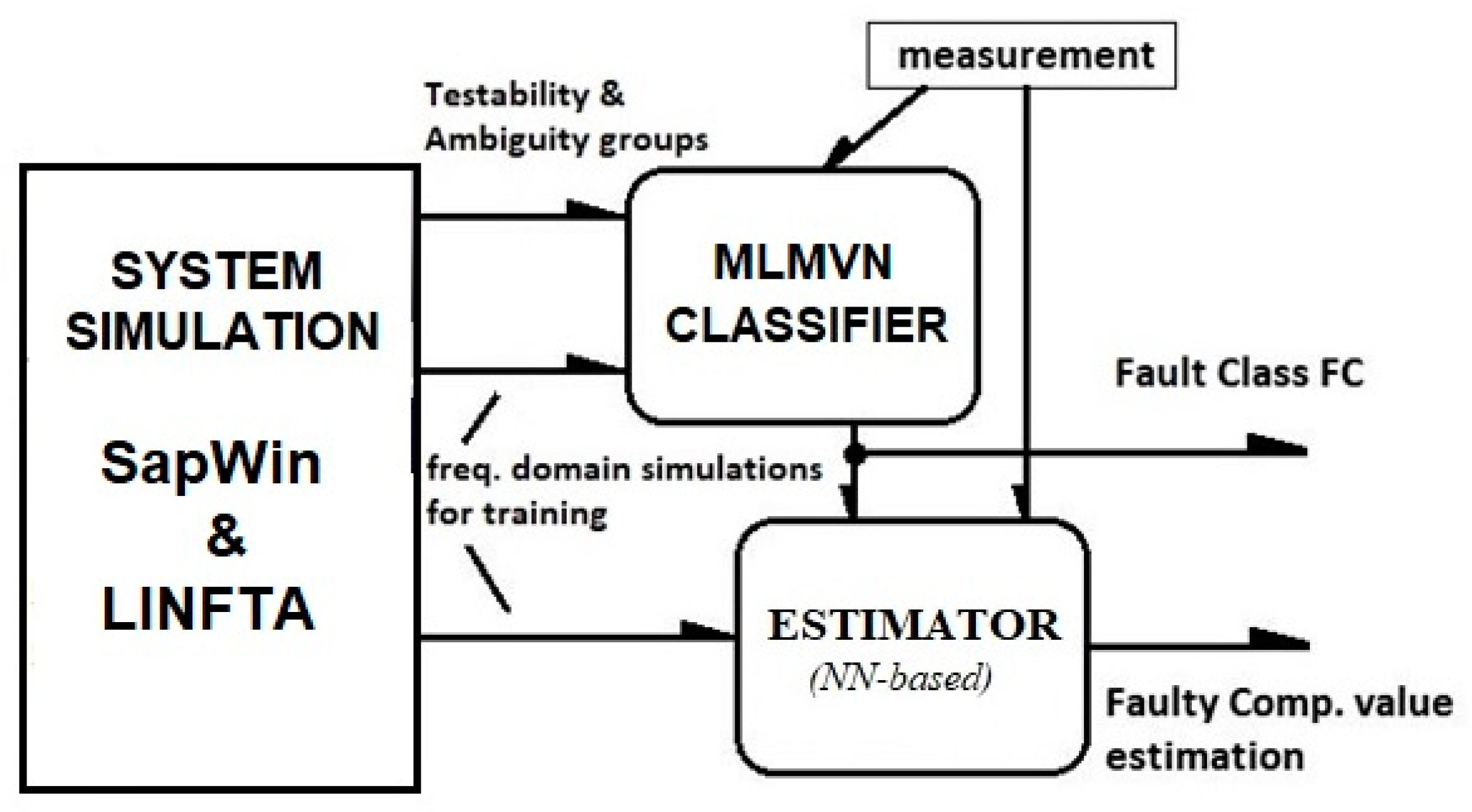
3. The Fault Diagnosis Procedure

The block diagram in Figure 1 summarizes the procedure. The function of each block is described in the following paragraphs.

3.1. Testability Analysis

The goal of the whole procedure is to interpret the multi-frequency measurements taken over the output terminals of the CUT (the test points) in order to locate which component is out of tolerance. A major drawback is due to the nonlinear nature of the problem, also for linear circuits. This happens because the parameters associated to the components appear as products in the coefficients $a_i$ and $b_j$ of the network function whose canonical form is the following:

$$H\left(\mathbf{p},s\right)=\frac{N\left(\mathbf{p},s\right)}{D\left(\mathbf{p},s\right)}=\frac{{\sum }_{i=0}^n\frac{a_i\left(\mathbf{p}\right)}{b_m\left(\mathbf{p}\right)}\cdot s^i}{s^m+{\sum }_{j=0}^{m-1}\frac{b_j\left(\mathbf{p}\right)}{b_m\left(\mathbf{p}\right)}\cdot s^j}.$$

(7)

Consequently, a set of two or more components are not distinguishable to each other starting from the measure of the output. An accurate evaluation of testability and ambiguity groups is a fundamental step for a correct fault diagnosis procedure, as confirmed in recent works [18,19,20], presenting efficient approaches to testability analysis. For analog circuits, in accordance with the definition proposed in the seminal paper [38], the testability (T) equates the solvability degree of the fault diagnosis equations. The maximum number of parameters identifiable starting from a given input-output set of measurements is the fault equation solvability degree and it is also the testability value T. T is never greater than the total number N of the potentially faulty CUT components; rather, it is very often less than N, and, consequently, it is useful to extract the “ambiguity groups” of the CUT. They are sets of components indistinguishable to each other [21]. Testability analysis consists of a testability evaluation and ambiguity group determination. Testability value establishes not only the maximum number of identifiable parameters but also the maximum allowed fault hypothesis, ambiguity groups give information on which parameters can be identified [21].

As shown in the next session, important definitions are the following two [21]:

• Canonic ambiguity group (CAG): an ambiguity group without any other ambiguity group (it is “minimum”);
• Global ambiguity group (GAG): an ambiguity group deriving from the union of two or more canonical ambiguity groups with at least one common element.

The testability analysis is performed by the program LINFTA [18].

3.2. Fault Classes and Fault Classification

Once the “solvability” of the CUT has been evaluated and the CAGs and GAGs have been determined, a classification method must be applied to the measurements in order to classify each measure in the correct “anomaly class”, which causes a malfunction and a deviation of the output. At this stage, a MLMVN classifier is in charge of providing the correct FC. As shown in [21,22,39], it is possible to consider a single component or a group of components for each FC. Assuming the single fault hypothesis, the identifiability of the circuit depends on the content of the GAGs: if all these groups are constituted by the union of CAGs of order at least equal to 3, the circuit is completely identifiable [21]. It should be noted that the order corresponds to the number of components belonging to a specific CAG and, consequently, the absence of CAGs containing 2 components makes the circuit completely identifiable. In this case, each parameter corresponds to a fault class. However, in the case of second order CAGs, it is not possible to uniquely identify the failure of the components belonging to these groups; this means that all the components not belonging to CAGs of order 2 are identifiable and each of them is a FC, while, for the components belonging to CAGs of order 2, there are two cases [22,39]:

• If there is null intersection between CAGs of order 2, then each of them is assumed to be a FC.
• If there is a non-null intersection between the CAGs of order 2, then each GAG given by the intersection of the CAGs of order 2 with non-null intersection is assumed as a FC.

In conclusion, the testability analysis, together with the single fault hypothesis, allows for the identification of the correct FC. Finally, every FC containing two or more components must be considered as a “unique” element. This means that, if a failure occurs in such an FC, it cannot be further distinguished which component of the class is actually faulty.

3.3. Fault Parameter Identification

The correct identification of the FCs is a fundamental stage and, in several situations, can be the only required information. The procedure proposed in this work gives a way to calculate them and, in case of ambiguity, it provides the set of components where the failure can occur. If the deviation of the faulty component with respect to its nominal value is required, once the error has been detected and located, the method is able to tune the solution with the module FINN (fault identification neural network), which provides an estimation of the value of the faulty component. If the FC is formed by multiple elements, an evaluation of the value can be obtained for each component (repeating the calculation for one component of the multiple FC at time, while keeping fixed the other ones).

4. Applications

To see how the whole procedure works, three circuits are considered in this section. Files of data used in these examples and appropriated description are available at Mendeley Data repository [40].

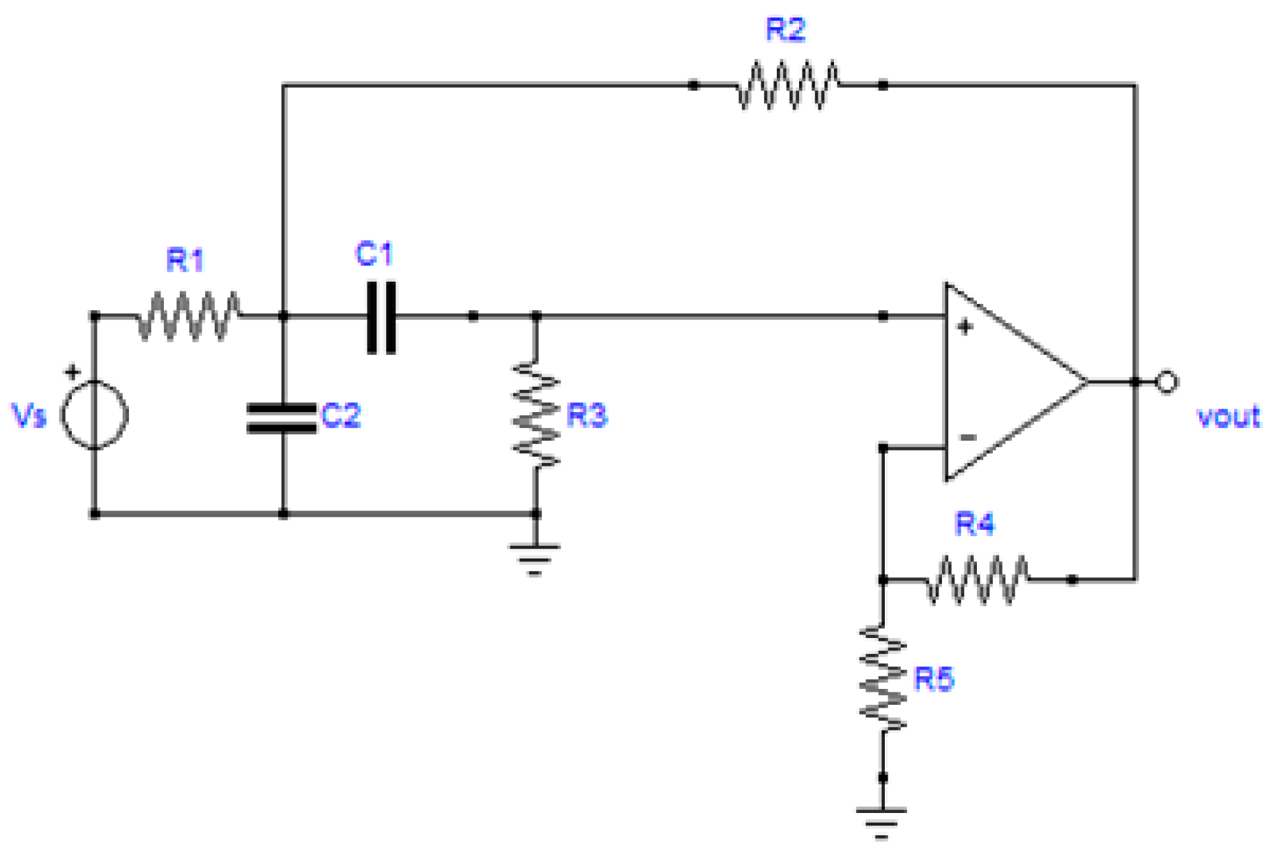
4.1. Sallen-Key Bandpass Filter

The Sallen-Key filter (SKF), shown in Figure 2, is a simple circuit with low sensitivity to the component variations, e.g., to the manufacturing tolerances. On the other hand, the low sensitivity makes it a challenging test for diagnosis, and it is also often used as a benchmark in fault diagnosis works (e.g., [22,26]). The used configuration is a bandpass centered at 25 kHz.

It includes 7 components that are potentially faulty, and the tolerances are assumed to be 10% for all the components (which is th same as in [26]), but now all components are considered. This is plausible because, as said before, SKF has a low sensitivity to large variations around nominal values. The analysis of testability of the CUT, conducted as outlined before, results in:

• Testability T = 3 (in relative percent 42.85%);
• Number of CAGs = 2 (1 CAG of order 2).

The only GAG is R4 and R5 (a CAG without any intersection with other CAGs can also be considered as a GAG).

The procedure described in Section 3.2 reveals that the FCs of the CUT are 6, related to the 5 two terminal components R1, R2, R3, C1, and C2 (then, each of them constitutes a FC); a further FC is constituted by the GAG (R4, R5). In the classification stage, the “not faulty” configuration is assumed as a further class, and it must be taken into account so that the final number of classes is 7.

The CUT is then simulated by SapWin, and the simulator provides the transfer function and, by exploiting it, generates the necessary set of simulated data in the following way:

• Multi-frequency: magnitude and phase are measured at 12 different frequencies; the number and the values of frequencies are chosen by exploiting the method developed by the authors in [32,33].
• Multi-parameter: starting from the nominal value, the component parameter is randomly varied in the tolerance range. As specified above, in this example the tolerance values are taken equal to 10% for all the components. A larger tolerance range makes the classification task more challenging.
• In each simulation, just a single component is randomly varied in the range (0.01 p_n–100 p_n), where p_n is the nominal value of the component.
• A set of simulations is generated with no fault element, in order to include also the class “0”, that is the circuit under nominal operating conditions.

The number of simulations is 1000, wherein 700 of them are used for training and 300 for failure classification.

In order to evaluate in a detailed way the performance of the fault diagnosis, we used the following terminology:

• False negative: number of cases in which there was a fault, but the system classified it as a no-fault case.
• False positive: number of cases in which there was no fault, but the classifier returned a fault in the circuit.
• Precision: the percent of cases that were actually faulty, among all the cases that actually were detected to be faulty.
• Fault diagnosability: the percent of cases which were correctly detected to have a fault, among all the fault cases.
• Accuracy: ratio of correctly classified test cases to all the test cases.

The results obtained with this method are compared with the best result coming from a SVM classifier, whose actual implementation of the code can be found on a recently presented SVM library [41]. SVM results were the best ones obtained until now.

The number of neurons used in a single hidden layer of the MLMVN classifier is established, in each case, by means of a heuristic procedure composed by two steps:

• The number of neurons is varied from $N_{min}$ to $N_{max}$ (typically 10–300, but it can be increased if the result is not clear, that is if there is not a maximum in the range), using an incremental step 10.
• The number of hidden layer neurons is refined in a neighborhood of the best number obtained at point 1 and ±20, using a step 2 at this time.

In

Table 1. Fault classification results in SKF.

	Training Set		Test Set
	MLMVN	SVM	MLMVN	SVM
False negative	(23/700) 3.29%	(24/700) 3.43%	(11/300) 3.67%	(12/300) 4.00%
False positive	(0/700) 0.00%	(3/700) 0.43%	(0/300) 0.00%	(3/300) 1.00%
Precision	100.00%	99.33%	100.00%	98.29%
Fault diagnosability	95.20%	94.87%	94.52%	93.48%
	Accuracy %
	MLMVN	SVM	MLMVN	SVM
Overall	92.86	93.86	91.67	90.00
0 (healthy)	100.00	98.71	100.00	97.41
1 (C1)	87.38	71.05	92.11	68.75
2 (C2)	96.51	98.65	90.91	97.30
3 (R1)	87.88	98.77	89.29	87.10
4 (R2)	96.00	95.52	89.66	86.67
5 (R3)	74.29	92.94	70.59	81.82
6 (GAG)	93.67	91.76	92.31	88.89

, the fault classification results for SKF are reported. The MLMVN classifier, which was used here, has 82 neurons in the hidden layer and 7 neurons in the output layer (6 FCs and the healthy class). Each of the output neurons performs “one vs. all” binary classification where each neuron is designated to classify a sample from its class and reject samples from all other classes. Thus, output neurons have discrete activation function dividing the complex plane into two sectors half-planes. The winner is determined by the closeness of the weighted sums for the output neurons to the bisector of the sector designated to classify a sample in terms of angular distance (that is, in terms of closeness of the argument of the weighted sum to $\pi /2$ or $3\pi /2$ depending on upper or bottom half-plane is designated to recognition of a sample). In almost all cases, the result is obtained using MLMVN, which is better than the one (already valuable) obtained using SVM. Thus, MLMVN outperforms SVM in terms of generalization capability. The dataset used for this simulation is contained in the text file entitled “SallenKey1000_12fClass” within the Supplementary Materials. Furthermore, the text file called “Readme” provides all the information to properly use this dataset.

Here, and in all other experiments, the number of hidden neurons in MLMVN was chosen experimentally as a minimum number ensuring the best result. The number of output neurons is equal to the number of classes in the classification problem to be solved.

After the phase of classification, the value assumed by a fault component can be extracted by using the FINN module. The identification of the value can be refined with further simulations: a set of 2000 simulations, divided into 1500 for training and 500 for test, is used for each component. Therefore, there is a set of MLMVNs, each dedicated to predicting the deviation of the single fault component. In this stage, the most important result is not to obtain the exact value of the component, but rather to predict the nature of the failure (i.e., small or large increase, small or large decrease). In this perspective, the obtained results can be highly acceptable also in terms of approximation of the real value of the faulty component over a so extended range; this is a consequence of using the preliminary classification phase, which results in a drastic reduction in the dimension of the space of the solutions on which the parameters of the neural network are moving. In

Table 2. Fault component identification results.

FC	Nominal Value	FCerr% (MLMVNN)
1 (C1)	5 × 10−9 F	17.12
2 (C2)	5 × 10−9 F	11.4
3 (R1)	5.18 kΩ	26.2
4 (R2)	1000 Ω	14.9
5 (R3)	2 kΩ	17.7
6 (GAG)	4 kΩ (R4–R5)	31.2

, the nominal values of the components and the results of identification are reported.

In the third column of the Table 2, the mean percent error over the possible failure for each FC is shown. It is defined as:

$$FCerr\%=\frac{1}{N_{test}}{\sum }_{i=1}^{N_{test}}\left|\frac{p_i^{\left(out\right)}-p_i^{\left(fault\right)}}{p_i^{\left(fault\right)}}\right|\cdot 100,$$

(8)

where $N_{test}$ is the number of test data samples (500 in this example), $p_i^{\left(out\right)}$ is the value provided by the FINN module for the FC parameter, and $p_i^{\left(fault\right)}$ is the value assumed by the faulty component. As it can be observed on the Table 2, there is a discrepancy among the results in term of percent error, in some FC the identification is precise enough, in some other much less. This fact essentially depends on the sensitivity of the used network function with respect to the given parameter, together with the large variation range which is used in this evaluation. On the other hand, it should be considered that, at this stage, also an error which is apparently huge can be considered more than acceptable for this task and over a large parameter variation range. Let us assume, for instance, a resistance with a nominal value 1 kΩ and a real (faulty) value of 10 kΩ, identified with an apparently huge error of 30%. This means that the error is associated by the FINN module to a value moving between 7000 and 13,000 Ω, which is a good estimate of the occurred failure.

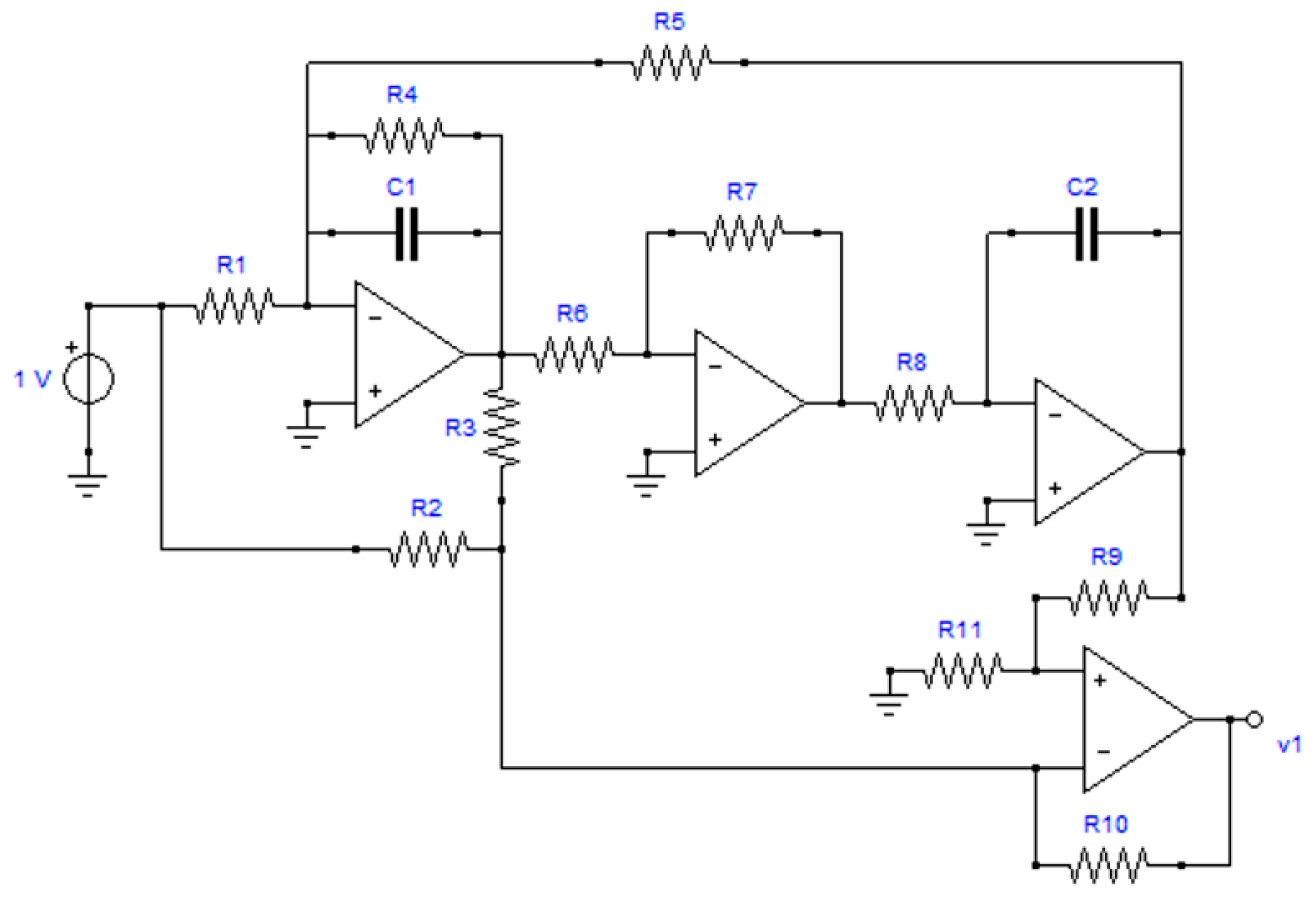
4.2. Lowpass Biquadratic Filter

An analog biquadratic LP filter, reported in Figure 3, is taken as a second case. In the circuit, 13 elements are present which could be subject to fail (R1-R11, C1, and C2), while an ideal model is used for the operational amplifiers.

The testability analysis of the CUT, performed as described above, returns the following results:

• Testability T = 5 (in relative percent 38.46%)
• Number of CAGs = 55 (among these, 7 CAGs have order 2)

There are two GAGs and they are:

• GAG1 = (R6, R7, R8, C2)
• GAG2 = (R9, R11)

All the resistances have a nominal assigned value of 1 kΩ, except R4 = 500 Ω, C1 = C2 = 100 nF. Again, the procedure detailed in Section 3.2 determines that the FCs of the CUT are 9, coupled to the 7 elements R1, R2, R3, R4, R5, R10, and C1 (each of them is a FC), with the addition of the two FCs GAG1 (constituted by the intersection of 6 CAGs of order 2) and GAG2. Considering also the “not faulty” circuit, the possible classes are 10.

The generation of samples is done in the same way of the previous example (in this case the total number of simulations is 2000; 1500 are used for training and 500 for failure classification), and in

Table 3. Fault classification results in active low pass filter.

	Training Set		Test Set
	MLMVN	SVM	MLMVN	SVM
False negative	(16/1500) 1.07%	(13/1500) 0.87%	(3/500) 0.60%	(8/500) 1.60%
False positive	(7/1500) 0.47%	(1/1500) 0.07%	(1/500) 0.20%	(1/500) 0.20%
Precision	99.21%	99.89%	99.66%	99.66%
Fault diagnosability	98.26%	98.61%	99.01%	97.38%
Accuracy %
	MLMVN	SVM	MLMVN	SVM
Overall	98.40	98.93	98.80	95.60
0 (healthy)	98.79	99.82	99.49	99.49
1 (C1)	100.00	100.00	100.00	100.00
2 (GAG1)	100.00	100.00	100.00	97.37
3 (R1)	100.00	100.00	100.00	96.30
4 (R10)	100.00	91.95	97.56	84.62
5 (GAG2)	88.28	92.47	84.21	76.47
6 (R2)	100.00	100.00	100.00	100.00
7 (R3)	97.96	99.12	96.77	91.89
8 (R4)	100.00	100.00	100.00	97.14
9 (R5)	100.00	100.00	100.00	97.30

, the results of train and test are reported. The MLMVN classifier used here has 80 neurons in a single hidden layer and 10 neurons in the output layer (9 FCs and the healthy class), also performing “one vs. all” classification. The dataset used for this simulation is contained in the text file entitled “LowPass2000_12fClass” within the Supplementary Materials. Furthermore, the text file named “Readme” provides all the information to properly use this dataset.

The classification rate is very good in almost all cases, with a slight decrease in the FC 5. Table 3 shows very similar classification results during the training phase, while a small difference can be seen in the testing phase. Since the data used for the tests are not processed during the training phase, this difference depends on the generalization capability of the methods. The complex neural network has several hyperparameters that can be set during the training phase and, for this reason, the structure of the classifier is more flexible and can be organized to increase the generalization capability. For example, the number of neurons in the hidden layer can be changed to improve the processing of new data while maintaining training performance. Furthermore, the soft margin technique shown in [28] is used to improve performance and increase generalization capability. In the same way of the previous example, also the identification stage is performed, and the results are reported in

Table 4. Fault component identification results.

FC	Nominal Value	FCerr% (MLMVNN)
1 (C1)	1 × 10−7 F	8.2
2 (GAG1)	1 × 10−7 F (C2)	9.6
3 (R1)	1000 Ω	62.6
4 (R10)	1000 Ω	51.0
5 (GAG2)	1000 Ω (R11)	47.1
6 (R2)	1000 Ω	2.3
7 (R3)	1000 Ω	38.5
8 (R4)	500 Ω	2.8
9 (R5)	1000 Ω	46.2

.

As can be observed in Table 4, the discrepancy among the results in term of percent error is still larger than in the previous case, but the general considerations about the results are not substantially modified and all kinds of deviation are correctly identified.

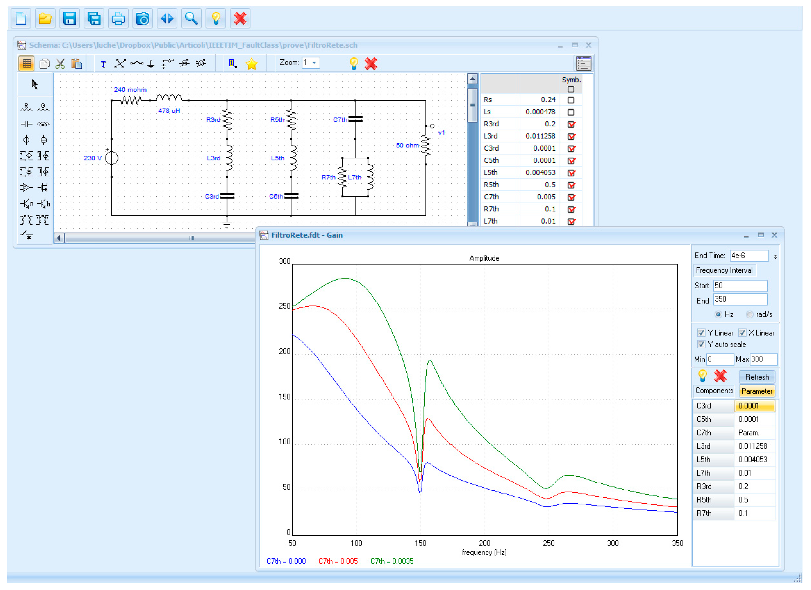
4.3. A Network Filter

The third example is a passive network filter, largely used in the low frequency distribution system, in order to suppress (or to mitigate) the disturbs over the line caused by the nonlinear loads (in recent years, this kind of noise has increased, mainly due to the switching converters and electrical drives connected to the line) [42]. In Figure 4, a schematic of the network filter is shown together with its frequency response curves. The filter is typically installed in a three-phase system, and each single phase is taken in consideration for the measurements. The filter under exam is constituted by three groups of R-L-C impedances connected across the line, with the goal of correctly attenuating the odd order harmonics on the line (the even harmonics are much less influential, since their contribution tends to cancel). The components of the impedances have the following names and nominal values:

• R3rd = 0.2 Ω; C3rd = 100 μF; L3rd = 11.258 mH;
• R5th = 0.5 Ω; C5th = 100 μF; L5th = 4.053 mH;
• R7th = 0.1 Ω; C7th = 5 mF; L7th = 10 mH.

The network is supplied by a generator with internal impedance Zs = 0.24 + j · 0.15 Ω.

The nine components of the filters are the elements of the CUT that are subject to failure. The testability analysis of the network gives, in this third example, the value T = 9 (the maximum possible), and the preliminary process is much simpler than in the first example, where there are no ambiguity groups. Thus, it is obvious that each electrical component also constitutes a FC.

In a similar way to the previous examples, the CUT is loaded into SapWin, which provides the network function for the multi-frequency/multi-parameter simulations:

• For each simulation, 7 frequencies are chosen, wherein magnitude and phase are measured; in this case, the used frequencies are those of 1st, 3rd, 5th, and 7th harmonics (in the range 50–350 Hz), increased by interposed samples.
• In this case, the tolerances are chosen following the typical specifications for this kind of filter, which is equal to 2% for capacitors and inductors and 5% for resistances.
• In each simulation, a single component value is randomly variated in the range (0.01 p_n–100 p_n), where p_n is the nominal value of the component.
• The total number of simulations is 4000; 2500 are used for training and 1500 for failure classification.

In

Table 5. Fault classification results in a network filter with no evaluation of the response.

	Training Set		Test Set
	MLMVN	SVM	MLMVN	SVM
False negative	(131/2500) 5.24%	(185/2500) 7.40%	(98/1500) 6.53%	(120/1500) 8.00%
False positive	(0/2500) 0.00%	(0/2500) 0.00%	(0/1500) 0.00%	(0/1500) 0.00%
Precision	100.00%	100.00%	100.00%	100.00%
Fault diagnosability	92.02%	88.73%	89.55%	87.21%
Accuracy
	MLMVN	SVM	MLMVN	SVM
Overall	93.68	88.28	89.80	87.33
0 (healthy)	100.00	100.00	100.00	100.00
1 (C3rd)	98.40	98.40	94.69	98.23
2 (C5th)	96.81	79.79	93.58	77.06
3 (C7th)	100.00	100.00	87.76	100.00
4 (L3rd)	90.51	87.34	84.00	78.00
5 (L5th)	98.56	86.54	94.90	85.71
6 (L7th)	44.28	40.80	29.41	28.43
7 (R3rd)	91.12	55.03	85.42	56.25
8 (R5th)	97.75	94.94	84.76	88.57
9 (R7th)	100.00	100.00	95.73	100.00

, the results are shown. In this table a worsening of the results can be noticed, with respect to the previous example, and this could appear counterintuitive, seen the higher number of simulations and the higher testability. The dataset used for this simulation is contained in the text file entitled “NetworkFilter4000_7fClass” within the Supplementary Materials. Furthermore, the text file called “Readme” provides all the information to use this dataset correctly.

When applying this method to a passive filter, in fact, the pure classification of “faulty state” as a state where a parameter is out of tolerance and is usually too weak to lead the classifier to a correct result. The rigorous evaluation of the testability and ambiguity component groups (and thus of the FCs) is mainly due to a couple of reasons:

• There was a low sensitivity of some parameters of the system and then a small variation in the space of the solutions. In Figure 5, for instance, the parametric magnitude sensitivities of L7th is shown, which were associated to the FCs with the worst result.

In this circuit, some components represented a parasitic (non-ideal) behavior, and it is not fully correct to talk about a faulty component, but rather about a deviation. The deviation of a parasitic resistance typically influences the output in just one direction. Consequently, in this case, a different approach to the concept of “failure” should be adopted in order to improve the classifier result. Therefore, in a second test, only those simulations that were over the range of response established by the specifications of the problem were considered faults. In practice, in this latter case, only the samples were kept in the classification set whose magnitude response was beyond a threshold of 20% deviation with respect to the requested values at the measured frequencies. This operation reduced the number of samples by about 20%, but drastically improved the classification result, as reported in

Table 6. Fault classification results in a network filter with evaluation of the response.

	Training Set		Test Set
	MLMVN	SVM	MLMVN	SVM
False negative	(1/2500) 0.04%	(0/2500) 0.00%	(2/824) 0.24%	(3/824) 0.36%
False positive	(0/2500) 0.00%	(0/2500) 0.00%	(0/824) 0.00%	(0/824) 0.00%
Precision	100.00%	100.00%	100.00%	100.00%
Fault diagnosability	99.94%	100.00%	99.63%	99.44%
Accuracy
	MLMVN	SVM	MLMVN	SVM
Overall	99.04	95.88	97.09	95.39
0 (healthy)	100.00	100.00	100.00	100.00
1 (C3rd)	97.55	94.12	95.08	93.44
2 (C5th)	100.00	84.51	98.48	89.39
3 (C7th)	100.00	100.00	98.88	100.0
4 (L3rd)	91.89	91.89	87.50	86.11
5 (L5th)	100.00	84.62	100.00	84.85
6 (L7th)	97.73	100.00	87.50	100.00
7 (R3rd)	100.00	100.00	98.25	98.25
8 (R5th)	100.00	100.00	90.70	88.37
9 (R7th)	100.00	100.00	95.38	98.46

. In order to make homogeneous the comparison with the results in Table 5, the same training conditions were considered and the reduction of the sample number was completely carried out in the test set, as can be noted in Table 6.

The MLMVN classifier used here has 230 neurons in a single hidden layer and 10 neurons in the output layer (9 FCs and the healthy class).

It is appropriate to consider the last results as the more interesting, because they combine the error over the component together with the effective consequence over the output of the CUT.

As in the previous example, once the classification concludes, the FINN program can be applied to the component, which may result in a faulty way in order to evaluate its value. The test is conducted in the same way of the previous examples and the results are reported in

Table 7. Fault component identification results.

FC	Nominal Value	Mean Error % (MLMVNN)
1 (C3rd)	1 × 10−4 F	7.9
2 (C5th)	1 × 10−4 F	25.1
3 (C7th)	5 × 10−4 F	7.7
4 (L3rd)	11.258 mH	48.1
5 (L5th)	4.053 mH	15.5
6 (L7th)	10 mH	36.2
7 (R3rd)	0.2 Ω	33.7
8 (R5th)	0.5 Ω	12.1
9 (R7th)	0.1 Ω	3.1

.

The same considerations of the previous example can be repeated in this case.

5. Conclusions

A framework to analyze and locate parametric faults in analog circuits was presented in this paper. It shows how a synergic use of an accurate testability analysis, complex-valued neural network MLMVN, sensitivity analysis, and a suitable choice of the test frequencies can implement an efficient fault diagnosis method under the single-fault hypothesis. The testability analysis allowed us to determine how many and which parameters could be diagnosed, as well as how to exactly determine possible FCs. The use of MLMVN as a classifier allowed to associate the faulty component to the corresponding FC in a very accurate way thanks to its great classification capability. The chosen kind of neural network, based on the MVN, has the important characteristic of being able to directly manage complex inputs in the frequency domain. Sensitivity analysis helps identify which parameters produce stronger effects on the output as a consequence of their variations, while a suitable choice of the test frequencies help minimize the effect of measurement errors and component tolerances.

A comparison of SVM and MLMVN was also presented in this paper. The SVM method was chosen because it represents the most used machine learning technique in the field of classification. Other diagnostic techniques have been previously examined and this work presents those that offer the best results. Further classification methods will certainly be addressed in future developments of this work, such as the introduction of unsupervised learning techniques. The extension of the numerical evaluation of the fault value to both parametric and catastrophic failures, and the application of the method to the multiple fault diagnosis, will be matter of a future work.

References

1. Cui, Y.; Shi, J.; Wang, Z. Analog circuit fault diagnosis based on Quantum Clustering based Multi-valued Quantum Fuzzification Decision Tree (QC-MQFDT). Measurement 2016, 93, 421–434. [Google Scholar] [CrossRef]
2. Liu, Y.; Zhang, Y.; Yu, Z.; Zeng, M. Incremental supervised locally linear embedding for machinery fault diagnosis. Eng. Appl. Artif. Intell. 2016, 50, 60–70. [Google Scholar] [CrossRef]
3. Luo, H.; Lu, W.; Wang, Y.; Wang, L.; Zhao, X. A novel approach for analog fault diagnosis based on stochastic signal analysis and improved GHMM. Measurement 2016, 81, 26–35. [Google Scholar] [CrossRef]
4. Rayudu, R.K. A knowledge-based architecture for distributed fault analysis in power networks. Eng. Appl. Artif. Intell. 2010, 23, 514–525. [Google Scholar] [CrossRef]
5. Tadeusiewicz, M.; Hałgas, S. A Method for Local Parametric Fault Diagnosis of a Broad Class of Analog Integrated Circuits. IEEE Trans. Instrum. Meas. 2018, 67, 328–337. [Google Scholar] [CrossRef]
6. Tan, S.C.; Lim, C.; Rao, M. A hybrid neural network model for rule generation and its application to process fault detection and diagnosis. Eng. Appl. Artif. Intell. 2007, 20, 203–213. [Google Scholar] [CrossRef]
7. Tang, X.; Xu, A.; Niu, S. KKCV-GA-Based Method for Optimal Analog Test Point Selection. IEEE Trans. Instrum. Meas. 2016, 66, 24–32. [Google Scholar] [CrossRef]
8. Tian, S.; Yang, C.; Chen, F.; Liu, Z. Circle Equation-Based Fault Modeling Method for Linear Analog Circuits. IEEE Trans. Instrum. Meas. 2014, 63, 2145–2159. [Google Scholar] [CrossRef]
9. Yang, C.; Yang, J.; Liu, Z.; Tian, S. Complex Field Fault Modeling-Based Optimal Frequency Selection in Linear Analog Circuit Fault Diagnosis. IEEE Trans. Instrum. Meas. 2013, 63, 813–825. [Google Scholar] [CrossRef]
10. Zhao, G.; Liu, X.; Zhang, B.; Liu, Y.; Niu, G.; Hu, C. A novel approach for analog circuit fault diagnosis based on Deep Belief Network. Measurement 2018, 121, 170–178. [Google Scholar] [CrossRef]
11. Bindi, M.; Grasso, F.; Luchetta, A.; Manetti, S.; Piccirilli, M. Modeling and Diagnosis of Joints in High Voltage Electrical Transmission Lines. J. Physics: Conf. Ser. 2019, 1304. [Google Scholar] [CrossRef]
12. Deng, Y.; Zhou, Y. Fault Diagnosis of an Analog Circuit Based on Hierarchical DVS. Symmetry 2020, 12, 1901. [Google Scholar] [CrossRef]
13. Binu, D.; Kariyappa, B. A survey on fault diagnosis of analog circuits: Taxonomy and state of the art. AEU Int. J. Electron. Commun. 2017, 73, 68–83. [Google Scholar] [CrossRef]
14. Spina, R.; Upadhyaya, S. Linear circuit fault diagnosis using neuromorphic analyzers. IEEE Trans. Circuits Syst. II Express Briefs 1997, 44, 188–196. [Google Scholar] [CrossRef]
15. Aminian, F.; Collins, H. Analog fault diagnosis of actual circuits using neural networks. IEEE Trans. Instrum. Meas. 2002, 51, 544–550. [Google Scholar] [CrossRef]
16. Aminian, M.; Aminian, F. A Modular Fault-Diagnostic System for Analog Electronic Circuits Using Neural Networks with Wavelet Transform as a Preprocessor. IEEE Trans. Instrum. Meas. 2007, 56, 1546–1554. [Google Scholar] [CrossRef]
17. Aminian, M. Neural-network based analog-circuit fault diagnosis using wavelet transform as preprocessor. IEEE Trans. Circuits Syst. II Express Briefs 2000, 47, 151–156. [Google Scholar] [CrossRef]
18. Fontana, G.; Luchetta, A.; Manetti, S.; Piccirilli, M.C. A Fast Algorithm for Testability Analysis of Large Linear Time-Invariant Networks. IEEE Trans. Circuits Syst. I Regul. Pap. 2017, 64, 1564–1575. [Google Scholar] [CrossRef]
19. Fontana, G.; Luchetta, A.; Manetti, S.; Piccirilli, M.C. An unconditionally sound algorithm for testability analysis in linear time-invariant electrical networks. Int. J. Circuit Theory Appl. 2015, 44, 1308–1340. [Google Scholar] [CrossRef]
20. Fontana, G.; Luchetta, A.; Manetti, S.; Piccirilli, M.C. A Testability Measure for DC-Excited Periodically Switched Networks with Applications to DC-DC Converters. IEEE Trans. Instrum. Meas. 2016, 65, 2321–2341. [Google Scholar] [CrossRef]
21. Fedi, G.; Manetti, S.; Piccirilli, M.C.; Starzyk, J. Determination of an optimum set of testable components in the fault diagnosis of analog linear circuits. IEEE Trans. Circuits Syst. I Regul. Pap. 1999, 46, 779–787. [Google Scholar] [CrossRef]
22. Cannas, B.; Fanni, A.; Manetti, S.; Montisci, A.; Piccirilli, M.C. Neural network-based analog fault diagnosis using testability analysis. Neural Comput. Appl. 2004, 13, 288–298. [Google Scholar] [CrossRef]
23. Fontana, G.; Grasso, F.; Luchetta, A.; Manetti, S.; Piccirilli, M.C.; Reatti, A. Testability Analysis Based on Complex-Field Fault Modeling. In Proceedings of the SMACD 2018—15th International Conference on Synthesis, Modeling, Analysis and Simulation Methods and Applications to Circuit Design, Prague, Czech Republic, 2–5 July 2018; pp. 33–36. [Google Scholar]
24. Cui, J.; Wang, Y. A novel approach of analog circuit fault diagnosis using support vector machines classifier. Measurement 2011, 44, 281–289. [Google Scholar] [CrossRef]
25. Grasso, F.; Luchetta, A.; Manetti, S.; Piccirilli, M.C.; Reatti, A. Single fault diagnosis in analog circuits: A multi-step approach. In Proceedings of the 5th IEEE Workshop on Advances in Information, Electronic and Electrical Engineering (AIEEE), Riga, Latvia, 24–25 November 2017; pp. 1–5. [Google Scholar] [CrossRef]
26. Vasan, A.S.S.; Long, B.; Pecht, M. Diagnostics and Prognostics Method for Analog Electronic Circuits. IEEE Trans. Ind. Electron. 2013, 60, 5277–5291. [Google Scholar] [CrossRef]
27. Du, B.; He, Y.; Zhang, Y. Open-Circuit Fault Diagnosis of Three-Phase PWM Rectifier Using Beetle Antennae Search Algorithm Optimized Deep Belief Network. Electronics 2020, 9, 1570. [Google Scholar] [CrossRef]
28. Aizenberg, I. MLMVN with Soft Margins Learning. IEEE Trans. Neural Netw. Learn. Syst. 2014, 25, 1632–1644. [Google Scholar] [CrossRef]
29. Aizenberg, I. Why We Need Complex-Valued Neural Networks? Geom. Uncertain. 2011, 353, 1–53. [Google Scholar] [CrossRef]
30. Aizenberg, I.; Luchetta, A.; Manetti, S. A modified learning algorithm for the multilayer neural network with multi-valued neurons based on the complex QR decomposition. Soft Comput. 2011, 16, 563–575. [Google Scholar] [CrossRef]
31. Aizenberg, I.; Moraga, C. Multilayer Feedforward Neural Network Based on Multi-valued Neurons (MLMVN) and a Backpropagation Learning Algorithm. Soft Comput. 2006, 11, 169–183. [Google Scholar] [CrossRef]
32. Grasso, F.; Luchetta, A.; Manetti, S.; Piccirilli, M.C. A Method for the Automatic Selection of Test Frequencies in Analog Fault Diagnosis. IEEE Trans. Instrum. Meas. 2007, 56, 2322–2329. [Google Scholar] [CrossRef]
33. Grasso, F.; Manetti, S.; Piccirilli, M.C. An approach to analog fault diagnosis using genetic algorithms. In Proceedings of the 12th IEEE Mediterranean Electrotechnical Conference (IEEE Cat. No.04CH37521), Dubrovnik, Croatia, 12–15 May 2004. [Google Scholar]
34. Aizenberg, E.; Aizenberg, I. Batch linear least squares-based learning algorithm for MLMVN with soft margins. In Proceedings of the 2014 IEEE Symposium on Computational Intelligence and Data Mining (CIDM 2014), Orlando, FL, USA, 9–12 December 2014; pp. 48–55. [Google Scholar]
35. Aizenberg, I. Hebbian and error-correction learning for complex-valued neurons. Soft Comput. 2012, 17, 265–273. [Google Scholar] [CrossRef]
36. Grasso, F.; Luchetta, A.; Manetti, S.; Piccirilli, M.C.; Reatti, A. SapWin 4.0-a new simulation program for electrical engineering education using symbolic analysis. Comput. Appl. Eng. Educ. 2015, 24, 44–57. [Google Scholar] [CrossRef]
37. Manetti, S.; Luchetta, A.; Piccirilli, M.C.; Reatti, A.; Grasso, F. Sapwin 4.0. Available online: www.sapwin.info (accessed on 29 January 2021).
38. Sen, N.; Saeks, R. Fault diagnosis for linear systems via multifrequency measurements. IEEE Trans. Circuits Syst. 1979, 26, 457–465. [Google Scholar] [CrossRef]
39. Grasso, F.; Luchetta, A.; Manetti, S.; Piccirilli, M.C. Symbolic techniques in neural network based fault diagnosis of analog circuits. In Proceedings of the XIth International Workshop on Symbolic and Numerical Methods, Modeling and Applications to Circuit Design (SM2ACD), Gammarth, Tunisia, 4–6 October 2010; pp. 1–4. [Google Scholar]
40. Luchetta, A. Analog Circuits. Available online: https://data.mendeley.com/datasets/64psx4vkh7/1 (accessed on 29 January 2021).
41. Chang, C.-C.; Lin, C.-J. LIBSVM: A library for support vector machines. ACM Trans. Intell. Syst. Technol. 2011, 2, 1–27. [Google Scholar] [CrossRef]
42. Akagi, H.; Watanabe, E.H.; Aredes, M. Instantaneous Power Theory and Applications to Power Conditioning; Wiley: Hoboken, NJ, USA, 2017. [Google Scholar]
Figure 1. Block diagram of the fault diagnosis system. MLMVN: multilayer neural network; LINFTA: linear invariant network fast testability analysis.
Electronics 10 00349 g001
Figure 2. Schematic of the Sallen₋Key filter (SKF).
Electronics 10 00349 g002
Figure 3. Schematic of the low pass filter.
Electronics 10 00349 g003
Figure 4. Network filter and magnitude response.
Electronics 10 00349 g004
Figure 5. Magnitude response sensitivity of L7th.
Electronics 10 00349 g005