Neural Networks for Driver Behavior Analysis

Abstract

The proliferation of info-entertainment systems in nowadays vehicles has provided a really cheap and easy-to-deploy platform with the ability to gather information about the vehicle under analysis. With the purpose to provide an architecture to increase safety and security in automotive context, in this paper we propose a fully connected neural network architecture considering position-based features aimed to detect in real-time: (i) the driver, (ii) the driving style and (iii) the path. The experimental analysis performed on real-world data shows that the proposed method obtains encouraging results.

1. Introduction

The Internet of things (IoT) is represented by the network of physical devices, home appliances, vehicles and a plethora of devices embedded with actuators, sensors, software and, in general, with connectivity [1]. Recently, Internet of Vehicle (i.e., IoT related to automotive) started to obtain more attention [2]. As a matter of fact, there are several promising benefits deriving from the real-world implementation of the Internet of Vehicle paradigm, for instance, a vehicle can turn from an autonomous and independent system into a component of a more efficient cooperative one [3].

Nowadays, vehicles can send data between them or to an external server in order to adapt the driving style to the road condition; traffic lights can send information about the number of cars in a lane in order to suggest to other cars an alternative path to avoid traffic congestion [4].

In this scenario the proliferation of both mobile devices and info-entertainment systems in modern cars, useful to gather features from vehicles while are travelling, boosted research community to focus about safety and security in the automotive context. In this scenario, data mining algorithms can be useful to analyse features collected from vehicles with the aim to extract knowledge related to the driver behavioral analysis.

For this reason, the main research trends in this topic are ranging from driver detection to driving style recognition.

With regard to driver detection (aimed to continuously and silently authenticate the driver to his/her car), the main aim is two-fold: anti-theft system (for end users) and a system for insurance companies proposing ad-hoc policies for the single driver.

New anti-theft paradigms are necessary, considering that cars are equipped with many computers on board, exposing them to a new type of attacks [5,6]. As any software, the operating systems running on cars are exposed to bug and vulnerabilities [7].

The driver detection is of interest also for auto insurance markets that are rapidly changing: through these plethora of new data easily available, risks can be rated on an individual basis; an insurer can now identify, measure and rate a particular person’s driving ability [8,9].

This idea is defined in the Usage Based Insurance (UBI) concept, introduced into the personal motor insurance market over a decade ago. Basically, it consists of two typical models: “pay as you drive” and “pay how you drive”. Premiums are based upon time of usage, distance driven, driving behavior and places driven to.

Relating to driving style recognition, this trend is more related to safety than driver detection but currently there are few studies proposing methods to address this issue.

In the context of intelligent cars, another topic of interest is related to the path detection able to suggest to drivers how to adapt the speed with regard to the kind of road traveled.

Several methods aimed to the driver detection exploit features gathered from Controller Area Network (CAN) bus, a vehicle bus standard designed to allow micro-controllers and devices to communicate with each other in applications without a host computer [10]. Through this bus passes a lot of information: from brake usage to fuel rate.

Different methods proposed in the current literature consider several sets of features extracted from the CAN bus. The problem is that from different vehicle manufacturers, different features are available (apart from a small subset common to all manufacturers): this is the reason why a method evaluated on a vehicle produced by a certain manufacturer it may not be available on a vehicle by another manufacturer or on a new version of the same vehicle. Furthermore, in order to exploit data from CAN bus, these methods need to have access to these data, and this can be resulting in a possible communication delay in a critical infrastructure like the one of the CAN bus or in any case when opening a channel on a bus containing extremely sensitive data, the channel will susceptible to an attack, as discussed in [11].

Starting from these considerations, in this paper we propose a method aimed to (i) discriminate between the vehicle owner and impostors, (ii) detect the driving style, and (iii) detect the kind of road traveled.

The proposed method considers a fully connected neural network architecture exploiting a feature vector based on positioning systems (i.e., we do not need to access to critical information CAN bus-related) in order to detect the driver, the driving style and the traveled road. So, the main contribution of the paper is the adoption of the same neural network architecture to solve these three different problems by exploiting the same feature set.

The main novelty of the proposed approach is represented by the silently and continuously real-time driver detection, the driving style monitor and the path detection. The driver detection is related to the detection of the vehicle owner useful, for instance, as anti-theft system but also for insurance companies that insure exclusively on a particular driver. The driving style is a tasks related to the safety, as a matter of fact it can be very useful to understand if a driver is changing his driving style, as happens for example in the case of drowsy or aggressive drivers. The identification of the road is useful to understand if the driver is traveling on a motorway road or a secondary one, to show consequently to the driver warnings relating to the moderation of speed and, in general, to invite him to adapt his driving style to traveled road.

Below we itemize the distinctive characteristics of the paper:

• we propose a method able to identify, exploiting the same feature set, the driver, the driving style and the kind of road traveled;
• we exploit a feature set easily obtainable (it does not require the access to the sensitive vehicle CAN bus);
• we designed and evaluate several fully connected neural networks and we find the optimal hidden layer number tuning for the driver identification task. Furthermore, using this configuration we demonstrate the neural network effectiveness in driving style and path recognition tasks;
• for experiment replicability, we consider two real-world datasets (where each instance is manually labelled by researchers with the relative driver, driving style and road) freely available for research purposes.

The paper proceeds as follows—Section 2 introduces preliminary notions about the neural network architecture considered in the following study, Section 3 deeply describes and motivates the proposed method; Section 4 illustrates the results of the experiments, Section 5 discusses the current literature related to driver behaviour characterization and finally, conclusions are drawn in Section 6.

2. Background

In this section we provide preliminary notions about neural network building blocks that is, the basis of each architecture neural network based.

One of the most important concept of neural network is represented by the so-called layer, a data processing module working as a filter for data. Basically, data are the layer inputs and they come out in a more useful form. Specifically, the layers are able to extract representations out of the data fed into them, representations that should be more meaningful for the problem to solve.

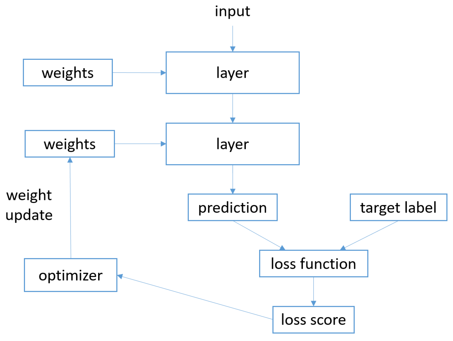
The neural network training consists in the definition of the following objects:

• layers: that are combined into the designed network;
• input data: the feature instances with the correspondent target labels;
• loss function: this function defines the feedback signal used for the learning;
• optimizer: the optimizer determines how the learning proceeds.

The interaction between the described objects are depicted in Figure 1.

The network aims to map the input data intro predictions and it is basically composed of layers together chained. The loss function compares the predictions with the target label, the result of this comparison is the loss value (i.e., a measure about how well the prediction of the network match was expected): this quantity is expected to be minimized during training [12]. Finally the optimizer uses the loss value to update the weights of the network: it determines how the network will be updated based on the loss function, usually it implements a specific variant of stochastic gradient descent.

As already introduced, the layer is the fundamental data structure—several layers are stateless, but there are several layers considering the state, in this case the layer exhibits weights which together contain the network knowledge. In the network design phase it is possible to choose between several layers, for instance, whether the input data are represented as vectors it is possible to use densely connected layers, while for image data 2D convolution layers are usually considered.

As an example, let us consider the following snippet:

layer = layers.Dense(32, input_shape = (784,))

The instruction represents the definition of a densely connected layers accepting a 784 sized vector and will return a 32 sized vector (a dense layer with 32 output units). As a consequence, the next layers will be declared in such a way that it is able to accept as input a 32 sized vector so building the layer chain.

The purpose of the layer is to transform the data. In the following we explain how these transformations can take place: a more complete declaration of the densely connected layers, previously considered, is the following one:

layer = layers.Dense(16, input_shape = (784,), activation = ’relu’)

The argument passed to densely connected layers is 16 in this case and it represents the number of hidden units of layers (an output 16 sized vector): formally a hidden unit is a dimension in the representation space of the layer.

In this layer the function able to “resize” the data has been specified (i.e., activation=’relu’ and it is called activation function). The layer can be interpreted as follows:

output = relu(dot(W, input)+b)

The output value is the combination of several operations: a dot product (i.e., dot) between the input vector and W (the weights of the layer) and an addition between the resulting vector and the bias (i.e., b). While the relu and the addition are element-wise operations, the dot operation combines entries (this is the operation that consents to the layer to “resize” the output data) [13]. Considering that W represents the actual value of weights for the considered layers (considering that the number of the weight is equal to the number of the neurons, for this reason whether we want to transform the data into a 16 size vector, the layer exhibits 16 weight, one weight for each neuron), while input represents the input feature vector.

Let us consider the following example in which there is a densely connected layer aimed to transform a 4 size vector into a 3 size one, where the input is $I=[2,3,5,6]$ and the weights are $W=[5,6,7]$, the dot product between I and W is:

$$\begin{array}{c}(5\times 2)+(5\times 3)+(5\times 5)+(5\times 6)\\ (6\times 2)+(6\times 3)+(6\times 5)+(6\times 6)\\ (7\times 2)+(7\times 3)+(7\times 5)+(7\times 6)\end{array}$$

the output of this layer is $O=[80,96,114]$: the layer resized the 4 size input data into a 3 size output data.

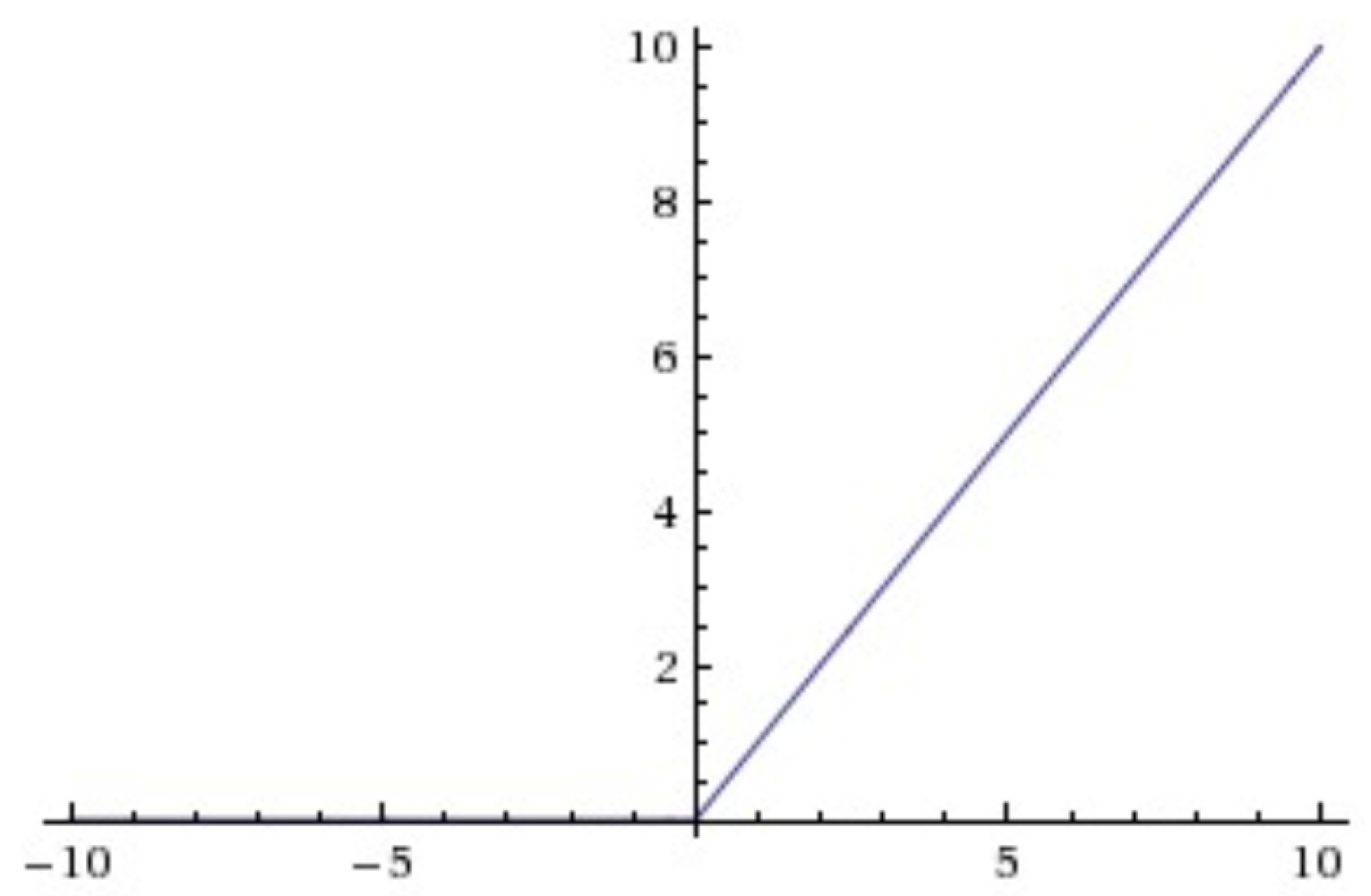
Finally, a relu (i.e., Rectified Linear Unit) operation (i.e., relu(x) = max (x,0)) is performed. For instance, with 4 hidden units, the dot product with W will project the input data onto a 4-dimensional representation space (to this we have to add the b bias vector and the relu operation). The relu trend is shown in Figure 2.

Basically the relu activation function is equal to zero when $x<0$ and it is linear with slope 1 when $x>0$. Considering more hidden units that is, an higher dimensional representation space, allows the network to learn more complex feature representations, but it makes the network more computationally expensive and may lead to learn unwanted data patterns (i.e., pattern that are improving the training data but not the testing ones).

From this discussion, it appears that the network designer in developing densely connected layers-based architecture have to choose: (i) how many layers to use and (ii) how many hidden layers to choose for each layer.

In addition the relu function, frequently considered as candidate for intermediate layers, another widespread activation function, the so-called softmax, is usually considered as last layer in classifiers neural network based before the output layer.

For instance, whether an instance under analysis can belong to one of the 4 label considered, it is possible to add following layer as final one:

layer = layers.Dense(4, activation = ’softmax’)

Coherently with the previously discussed example, the input from the previous layer is resized in a 4 size vector, the only difference is that the resizing is done using the softmax function and not the relu one.

The reason why the softmax activation function is considered as last layer before the output one is that its aim is to normalize an input vector into a probability distribution: it is usual that vector can exhibit negative or greater than one values. In order to have a feature vector which elements summed are equal to one we apply the softmax function. For instance whether the output of the previous densely connected layer with the softmax activation function is equal to $[0.2,0.1,0.4,0.3]$ this is symptomatic that the instance under analysis is belonging to the #3 class (the first element of the output vector presents the probability that the instance is belonging to the first class and so on).

3. The Driver Behavior Analysis Approach

In this section we describe in detail the high-level architecture and the method we proposed aimed to: (i) driver identification, (ii) detect the driving style and (iii) travelled road detection.

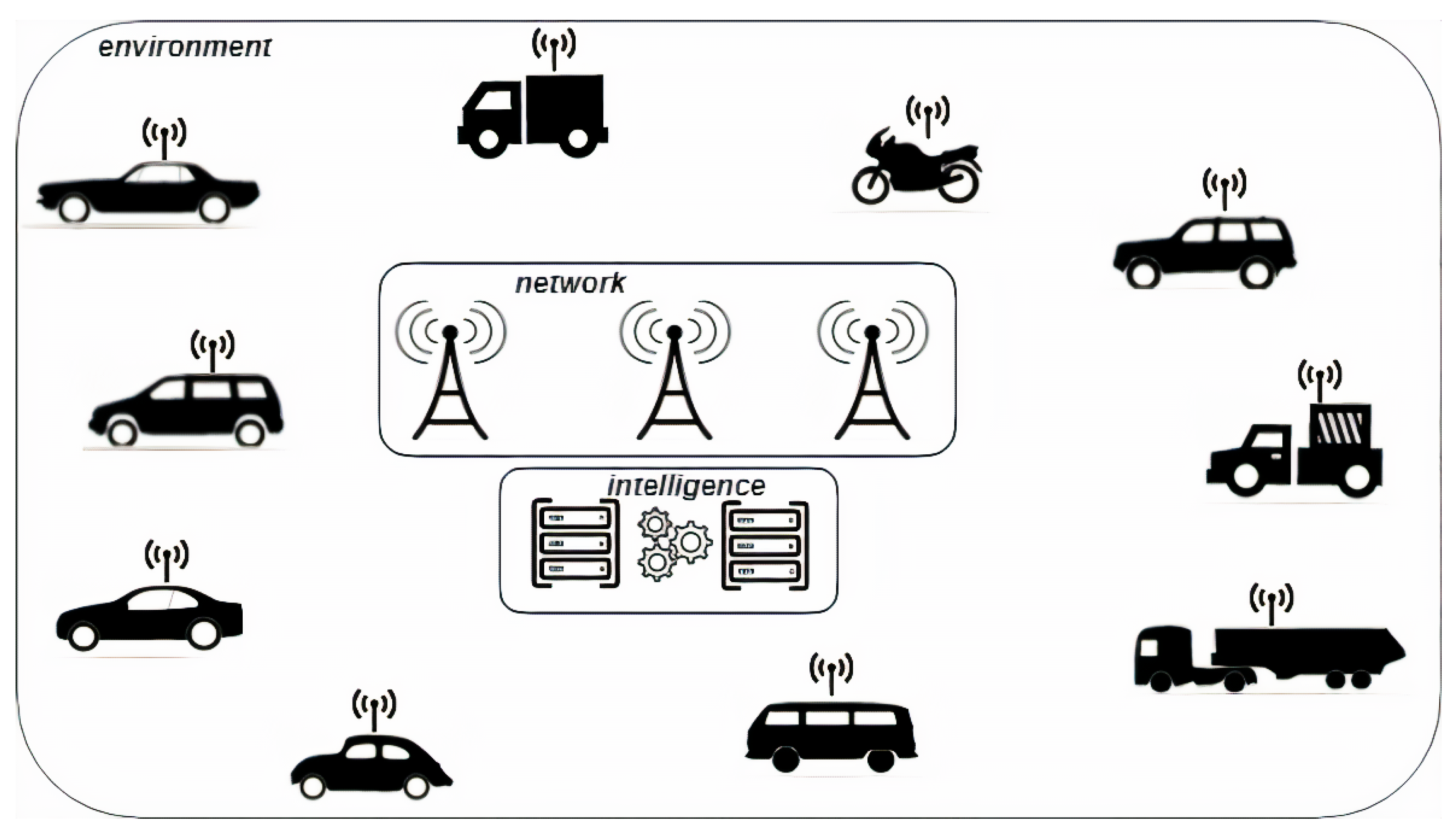
Figure 3 depicts the high-level architecture of the proposed method.

We distinguish three main blocks in Figure 3:

• intelligence: it represents the module able to store data and to compute the three different indicators for each driver. Once computed the indicators (related to the driver, the driving style and the road), this module is able to send suggestions to drivers for instance, in order to change the driving style to avoid traffic congestions. In addition the module is able to understand whether a vehicle is driven by the owner (to identify whether a theft is happened);
• network: this module represents the communication infrastructure of the proposed architecture;
• environment: this block depicts the environment, in which each vehicle is able to send a set of information related to its position. Considering that we use information related to the accelerometer sensor, the proposed method works on any type of vehicles (i.e., cars, trucks and motorcycles), without differences from the method performances point of view. Furthermore, only a mobile device (with a fixed-support) is required to obtain the information to send to the network module (alternatively it is also possible to send the accelerometer information using the info-entertainment system whether available in the vehicle).

In the following we describe in detail the proposed method to analyse the driver using data retrieved by positioning systems that is, the intelligence block in the architecture depicted in Figure 3.

We consider a set of features available from accelerometer, as shown in

Table 1. Features involved in the study.

Feature	Description	Measured in
F1	Acceleration in X	(Gs)
F2	Acceleration in Y	(Gs)
F3	Acceleration in Z	(Gs)
F4	Acceleration in X filtered by KF	(Gs)
F5	Acceleration in Y filtered by KF	(Gs)
F6	Acceleration in Z filtered by KF	(Gs)
F7	Roll	(degrees)
F8	Pitch	(degrees)
F9	Yaw	(degrees)

.

The feature set depicted in Table 1 contains the data available from the inertial sensors (available on mobile phones and on info-entertainment systems) at 10 Hz (reduced from the phone 100 Hz by taking the mean of every 10 samples). With the aim to gather data, the mobile device is fixed on the windshield at the start of the travel, in this way the axes are the same during the whole trip. These are aligned in the calibration process, being Y aligned with the lateral axis of the vehicle (reflects turnings) and Z with the longitudinal axis (positive value reflects an acceleration, negative a braking). The accelerometer measurements are logged filtered using a Kalman Filter (KF) [14]. KF is an algorithm exploiting a series of measurements observed over time, containing statistical noise and other inaccuracies, and produces estimates of unknown variables that tend to be more accurate than those based on a single measurement alone, by estimating a joint probability distribution over the variables for each timeframe: a common application is for guidance, navigation, and control of vehicles, particularly aircraft and spacecraft [15].

We considered a real-environment and not a simulated one in order to take in account all possible real-world variables, for instance, slowdowns traffic lights and all the possible variables that are not considerable from simulated environments. We highlight that the proposed feature set can also be easily collected from cheap mobile devices equipped, for instance, with the Android operating systems, but also from the info-entertainment systems available in modern vehicles.

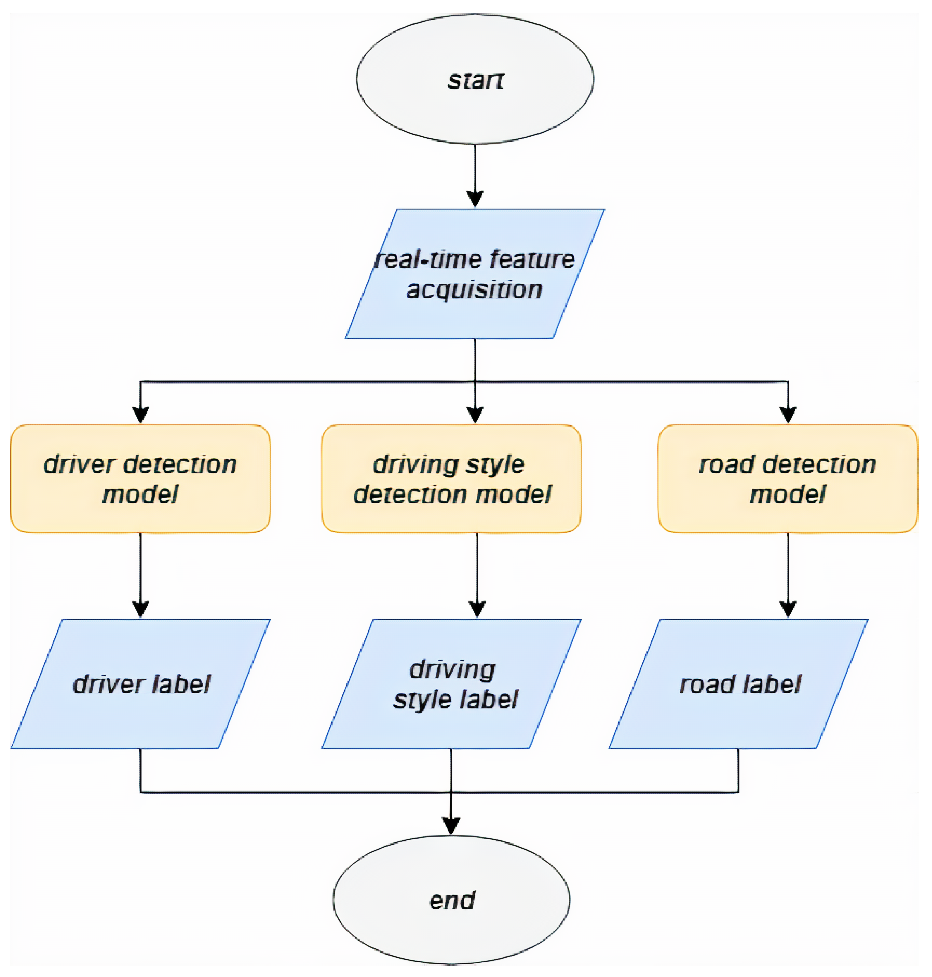
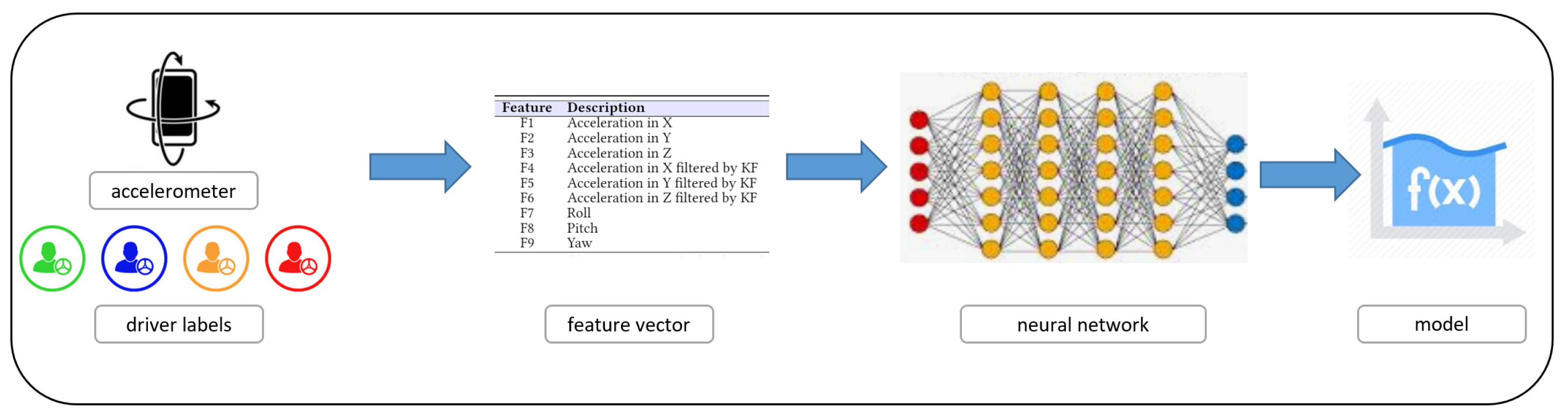
Figure 4 depicts the flow diagram of the intelligence module in detail:

• the real-time feature acquisition is the module responsible to gather the feature vector from the accelerometer sensor of the positioning systems (for instance the mobile device or the info-entertainment system built-in the vehicle);
• the driver detection model is the module able to test the feature vector obtained in the previous step against to the model to detect the driver;
• the driving style detection model is the module able to test the feature vector obtained in the previous step against to the model to detect the driving style;
• the road detection model is the module able to test the feature vector obtained in the previous step against to the model to detect the kind of road travelled;
• the driver label module contains the output of the prediction obtained in the driver detection model that is, the label related to the driver;
• the driver style label module contains the output of the prediction obtained in the driving style detection model, that is, the label related to the style (i.e., normal, aggressive or drowsy);
• the road label module contains the output of the prediction obtained in the road detection model that is, the label related to the style (i.e., secondary or motorway).

3.1. The Classification Process

We consider supervised techniques. To build models we consider the following three main steps: (i) data instances pre-processing (data cleaning and labeling), (ii) training neural networks with an increasing number of hidden layers and (iii) classification performance assessment (Testing).

The first step (i.e., pre-processing) consists in the cleaning of the raw instances of the feature by removing incomplete and wrong instances.

The second one, the Training, is depicted in Figure 5: starting from the data (in this case the features gathered from accelerometer), these algorithms generate an inferred function. The inferred function, provided by the neural network, should be able to discriminate between accelerometer features belonging to several classes, that is, the function should define the boundaries between the numeric vectors belonging to several classes.

In this study, the classes to discriminate are those related to drivers, the driver behaviours and kind of roads. One limit about the quality of the inferred function, and therefore of the supervised machine learning techniques, is related to the training data; it is important that the data used to build models are free of bias, in order to generate models able to predict the right class for unseen instances.

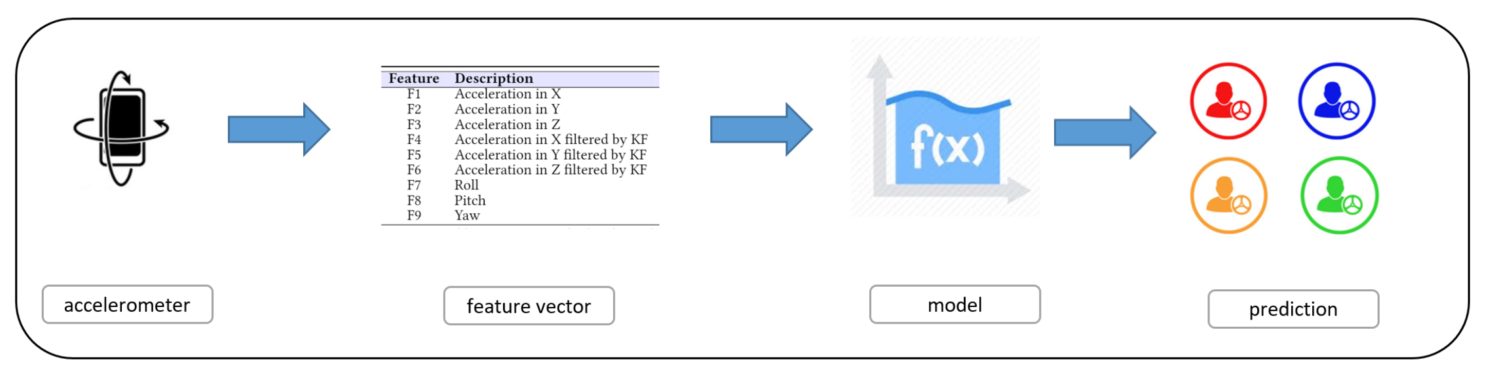
The third step, once generated the model is the evaluation of its effectiveness—the Testing one, is depicted in Figure 6.

The effectiveness of the models is measured using well-know information retrieval metrics. It is important to evaluate instances not included into the training data in order to evaluate the (real) performance of the built models. To assure this, we consider the cross validation—we split the full dataset in two parts and we used the first part as training dataset and the second one as testing dataset. We repeat this process considering different instances for both training and testing dataset in order to evaluate all the instances belonging to the full dataset.

Different models are defined—the first one for the driver detection, the second one for the driving style detection, while the third one is related to road identification: we highlight that each classification considers the same accelerometer feature set. To train the classifiers, with regard to the driver detection, we defined T as a set of labeled traces (M, l), where each M is associated to a label l ∈ {$U_1$,…,$U_n$} (where $U_n$ represents the n-th driver under analysis that is, Driver #n, with $1\le n\le 16$). For the second classifier, for the driving style detection we defined T as a set of labeled traces (M, l), where each M is associated to a label l∈ {$U_1$,…,$U_n$} (where $U_n$ represents a different driving style that is, Normal, Drowsy and Aggressive). Relating to the road identification classifier, we defined T as a set of labeled traces (M, l), where each M is associated to a label l∈ {$U_1$,…,$U_n$} (where $U_n$ represents the kind of road considered that is, Secondary and Motorway).

For each M the process calculates a feature vector V${}_f$ that is presented to the classifier during training.

In order to perform assessment during the training step, a k-fold cross-validation is used [16]: the dataset is subdivided into k subsets using random sampling. A subset is retained as a validation dataset to assess the trained model whereas the remaining $k-1$ subsets are exploited to perform training. Such process is repeated $k=5$ times—during the ten iterations, each of the k subsets has been used once as the validation dataset. To obtain a single reliable estimate, the final results are evaluated by computing the average of the results obtained during the ten iterations. The process starts by partitioning the dataset D in k slices. Then, for each iteration i, we train and evaluate the effectiveness of the trained classifier following the steps reported below:

(1)

the training set $T_i\subset$ D is generated by selecting an unique set of k − 1 slices from the dataset D;

(2)

the test set $T_i^{\prime }=D-T_i$ is generated selecting the remaining kth slice (it can be evaluated as the complement of $T_i$ to D)

(3)

a classifier is trained on set $T_i$;

(4)

the trained classifier is applied to $T_i^{\prime }$ to evaluate accuracy.

Since $k=5$, each iteration i is performed using the 80% of the dataset D as the training set ($T_i$) and the remaining 20% as test set ($T_i^{\prime }$).

The last step consists of using the trained classifiers on real user data to assess their performances. The aim is to identify the driver under analysis (with the first model), the driving style (with the second model) and the road (with the third model) in real-time, the adopted features model and feeding with it the trained classifier. The classification, in this study, is also performed by using a traditional machine learning approach based on decision trees (i.e., J48) with the aim of evaluating the performance improvement of the proposed neural network classifier with respect to the existing machine learning approaches (that do not use hidden layers).

3.2. The Neural Network Architecture

To build the three models related to the driver detection, driving style detection and road detection we design a neural network architecture.

The neural network architecture we propose in detail consists of a variable number of k hidden layers, with $min\le k\le max$ where min and max are, respectively, the minimum and the maximum number of hidden layers. We consider a different number of layers because in the evaluation section, we will experiment with several hidden layers with the aim to obtain the best performances for the driver detection task. Once the network is set up, the best architecture for the driver detection task will be used for the driving style detection and for the road detection tasks. The supervised classification approach described, aimed to generate the classifier model, is built considering a neural network architecture and is basically composed by following layers:

• Input layer: this layer is used as an entry point into the network, there is a node for each considered feature;
• Hidden layers: these layers are composed of artificial neurons (for instance, perceptrons). For each artificial neuron, the output is computed as a weighted sum of its inputs and passed through an activation function (that can be a sigmoid, a ReLu or a soft plus function).
• Dropout layer: this layer implements a regularization technique, which aims to reduce the complexity of the model with the goal to prevent over-fitting. Basically, this layer randomly deactivates several neurons in a layer with a certain probability p from a Bernoulli distribution. The reduced network is trained on the data in each stage and the deactivated nodes are reinserted into the network with their original weights. In the training stages, the “drop” probability for each hidden node is usually in the range [0, 0.5] (for this study 0.5 was used because dropping a neuron with 0.5 probability gets the highest variance for the distribution).
• Batch Normalization: Batch normalization [17] is a method for improving the training of feed-forward neural networks. It allows to obtain speed improvements and enables the adoption of higher learning rates, more flexible parameter initialization, and saturating non-linearities. We adopted this approach since batch normalized models achieve higher accuracy on both validation and test, due to a stable gradient propagation within the network.
• Output layer: this is the last layer of neurons that produce given outputs. We used a dense layer, exploiting a linear operation in which every input is connected to every output.

The MLP was trained by using cross-entropy [18] as a loss function, and stochastic gradient descent (SGD) for optimizing the loss function. Clearly, once obtained the best network configuration for the driver detection tasks (by training the network with the driver label, the same network is considered for the driving style (by considering the driving style labels) and road detection (by considering the road labels).

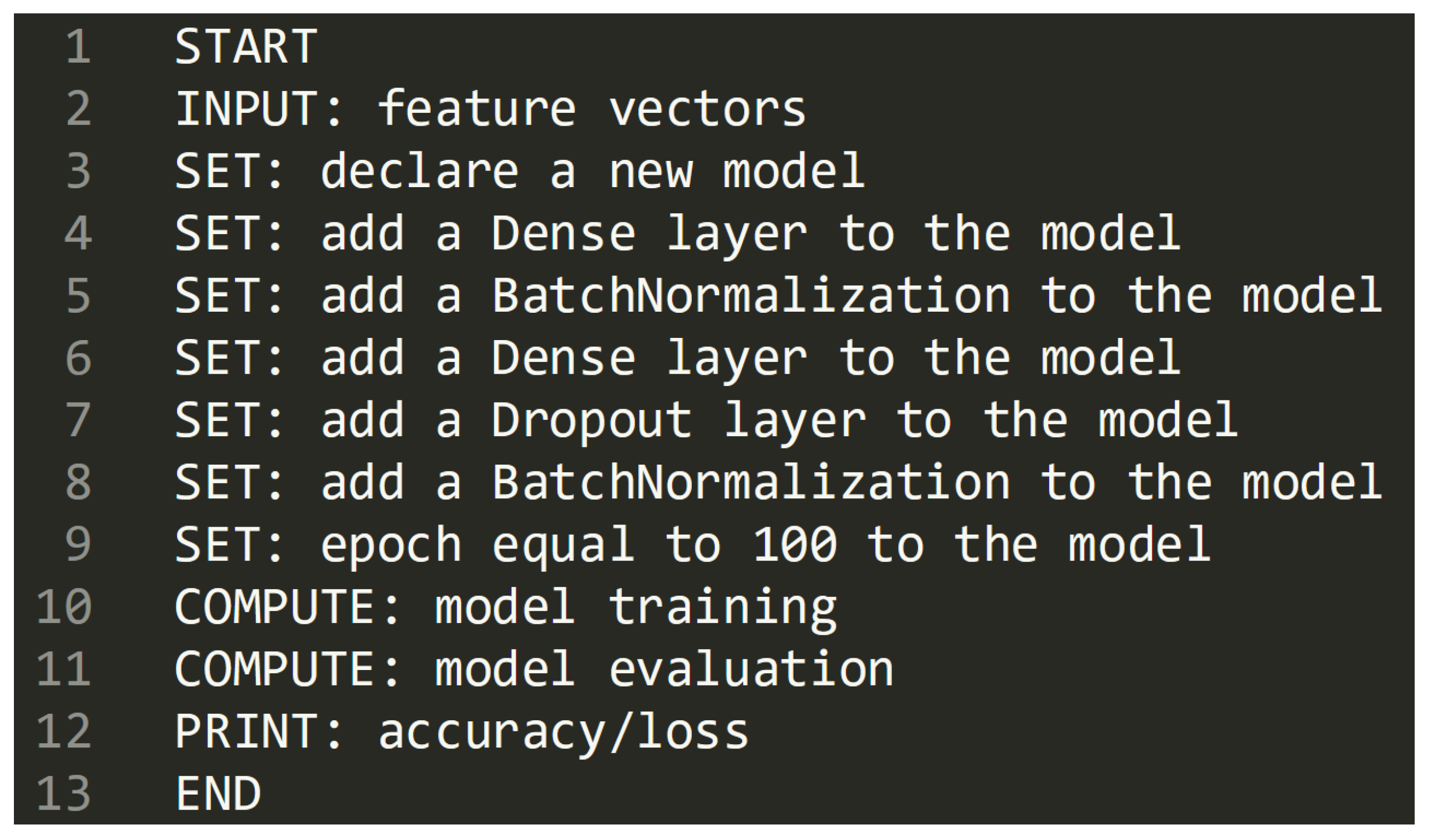
In Figure 7 we show the pseudocode related to the designed neural network implementation.

In the pseudocode in Figure 7 from line 5 to line 7 there is the Hidden layer implementation (the one that we repeat in order to tune the network).

For the network implementation, the Python programming language in considered. Moreover, the Tensorflow (https://www.tensorflow.org/) and the Keras (https://keras.io/) libraries are exploited. TensorFlow is an open source software library for machine learning, providing proven and optimized modules, useful in building algorithms for different types of artificial intelligence tasks. From the other side Keras is an open source library for machine learning and neural networks. It is written in the Python programming language and it is designed as an interface at a higher level of abstraction than other similar lower level libraries. It supports TensorFlow libraries as a back-end.

3.3. Study Design

We design an experiment aimed to investigate whether the feature set we consider is useful to discriminate between different drivers, different driving style and different roads using the proposed neural network architecture.

In detail, the experiment is aimed at verifying whether the considered features are able to predict unseen driver instances, unseen driving style and unseen road instances. The classification is carried out by using the neural network described in the previous section with the 9 features gathered from accelerometer as input neurons.

The evaluation consists of three stages: (i) a comparison of descriptive statistics of the populations of different drivers, driving styles and roads instances; (ii) hypotheses testing, to verify whether the features have different distributions for the considered driver populations; and (iii) a classification analysis aimed at assessing whether the considered features are able to correctly discriminate between different drivers, driving styles and roads related instances.

Each layer in the neural network is used to identify a unique feature of an instance under analysis [12]. Each layer will pick out a particular feature to learn and use it to classify the instance, for this reason we do not perform a feature selection but anyway we consider descriptive statistics and hypothesis testing to respectively provide a graphical and statistical impact about the effectiveness of the proposed feature vector.

To compare the driver, driving style and road instance populations through descriptive statistics we consider boxplot, a method for graphically depicting groups of numerical data through their quartiles. Boxplots represent variation in samples of a statistical population without making any assumptions of the underlying statistical distribution.

With regards to the hypotheses testing, the null hypothesis to be tested is:

$H_0$: ‘different drivers have similar values for the considered features’.

The null hypothesis was tested with Wald-Wolfowitz (with the p-level fixed to 0.05) and with Mann-Whitney Test (with the p-level fixed to 0.05). We chose to run two different tests in order to enforce the conclusion validity.

The purpose of these tests is to determine the level of significance, that is, the risk (the probability) that erroneous conclusions be drawn: in our case, we set the significance level equal to 0.05, which means that we accept to make mistakes 5 times out of 100.

4. Experimental Evaluation

In this section we describe the real-world dataset considered in the evaluation of the proposed method and the results of the experiment.

To implement the designed neural network architecture, we considered Tensorflow (https://www.tensorflow.org/), an open source software library for high-performance numerical computation and Keras (https://keras.io/), a Python-based high-level neural networks API, able to run on top of TensorFlow. Furthermore the Matplot (https://matplotlib.org/) library is considered as plotting library. We developed the network using the Python programming language.

The results of the evaluation are presented reflecting the data analysis’ division in three phases discussed in previous section: descriptive statistics, hypothesis testing and classification.

The metrics that are used to evaluate the classification results are the following: Precision, Recall, ROC Area, Accuracy and Loss.

Precision has been evaluated as the proportion of the examples that truly belong to a given driver among all those which were assigned to him/her. It is computed as the ratio of the number of relevant retrieved records (true positive) to the total number of irrelevant retrieved records (false negative) and relevant retrieved records (true positive):

$$\mathrm{Precision}=\frac{tp}{tp+fp}$$

where tp is the number of true positives and fp is the number of false positives.

The recall has been evaluated as the proportion of examples assigned to a given driver among all the instances that truly belong to the driver. It is computed as the ratio of the number of retrieved relevant instances (true positive) to the total number of relevant instances (the sum of true positive and false negative):

$$\mathrm{Recall}=\frac{tp}{tp+fn}$$

where fn is the number of false negatives.

The ROC Area is a measure of the probability that a positive example selected randomly is classified above a negative one.

The accuracy of a measurement system is the degree of closeness of measurements of a quantity to that quantity’s true value: it is the fraction of the classifications that are correct and it is computed as the sum of true positives and negatives divided all the evaluated instances:

$$\mathrm{Accuracy}=\frac{tp+tn}{tp+fn+fp+tn}$$

where tp indicates the number of true positives, tn indicates the number of true negatives, fn indicates the number of false negatives, fp indicates the number of false positives.

The Loss is a quantitative measure of how much the predictions differ from the actual output (i.e., the label). Loss is inversely proportional to the correctness or the model.

The loss is calculated on training and validation and its interpretation is how well the model is doing for these two sets: it is a summation of the errors made for each example in training or validation sets.

The machine used to run the experiments and to take measurements was an Intel Core i7 8th gen, equipped with 2GPU and 16Gb of RAM.

4.1. The Datasets

The datasets considered in the evaluation were gathered from a smartphone fixed in the car using an adequate support [14,19].

We collected data from two different datasets: the first one [14] considering six drivers, the second one [19] related to the data of ten different drivers.

A total of sixteen drivers participated to the experimental analysis, in

Table 2. Details about six drivers involved in the study with details about the genre, the age and the vehicle model.

Driver	Genre	Age Range	Vehicle Model
D1	Male	40–50	Audi Q5 (2014)
D2	Male	20–30	Mercedes B180 (2013)
D3	Male	20–30	Citroen C4 (2015)
D4	Female	30–40	Kia Picanto (2004)
D5	Male	30–40	Opel Astra (2007)
D6	Male	40–50	Citroen C-Zero (2011)

for reasons of space we show details about six of the drivers involved in the experiment (the ones gathered from the first dataset) [14]).

The full dataset we consider in the experimental analysis consist in more than 1000 min of naturalistic driving with its associated labels about the driver (i.e., from Driver #1 to Driver #16), the driving style (i.e, Normal, Drowsy and Aggressive) and the road (i.e., Secondary, Motorway).

The three driving styles (Normal, Drowsy and Aggressive) were performed in two different routes, one is 25 km (round trip) in a Motorway type of road with normally 3 lanes on each direction and 120 km/h of maximum allowed speed, and the other is around 16 km in a Secondary road of normally one lane on each direction and around 90 km/h of maximum allowed speed. The dataset publicly available for research purpose at the following urls: http://www.robesafe.com/personal/eduardo.romera/uah-driveset/ and https://github.com/martinacimitile/Car-Data-Mining/wiki. Each instance of the datasets is manually marked by researchers in [14,19] with three labels: the driver, the driving style and the road.

4.2. Descriptive Statistics

The analysis of boxplots helps to identify whether the features are helpful to discriminate between different drivers.

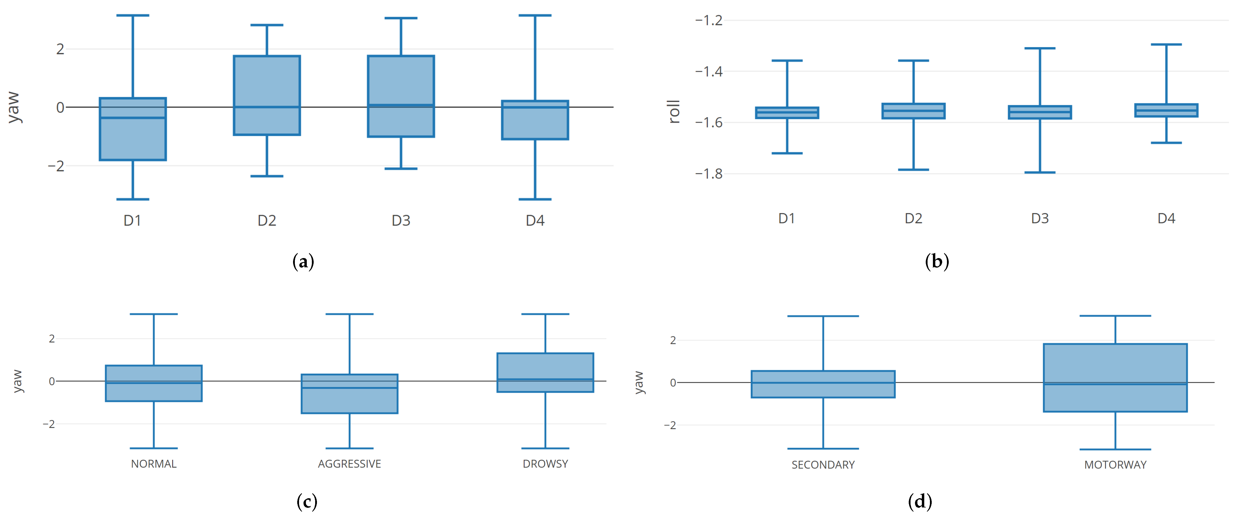
For space reasons, Figure 8 shows the boxplots related to the distributions of the considered features between the first 4 drivers involved in the experiment.

For reasons space, we do not represent all the boxplots but the same consideration can be provided for the remaining features.

The “(a)” box shows the boxplot related to the F9 feature (i.e., yaw): we notice that D2 and D3 drivers exhibits a similar boxplot, while D4 boxplot is smaller if compared with the one exhibit by D1 driver.

The “(b)” box shows the boxplot for the F7 feature (i.e., roll), from the point of view of these distributions we can highlight the boxplot related to the four driver are similar, but the D4 driver exhibits an higher maximum if compared with the other drivers.

The “(c)” box is related to the boxplot for the F9 feature (i.e., yaw) for driving style identification. From this boxplot we can see that the with regard to the drowsy boxplot, this is one is higher that the remaining ones (i.e., normal and aggressive).

The “(d)” box is related to the boxplot for the F9 feature (i.e., yaw) for road detection. The motorway boxplot exhibits a bigger range of values (between the first and the third quartile) if compared to the secondary one.

4.3. Hypothesis Testing

The hypothesis testing is aimed to evaluate whether the considered features exhibit different distributions for the populations of different feature belonging to the drivers with statistical evidence.

We assume valid the results when the null hypothesis is rejected by both the performed tests.

To summarize, considering that we assume the results valid when the null hypothesis is rejected by both performed tests, all the considered features passed both the tests (p < 0.001), symptomatic that the full feature vector can be suitable to discriminate between drivers, as the classification analysis will confirm.

4.4. Classification Analysis

In the following, we present the classification results obtained from both the neural network and machine learning classification approaches (considered as baseline) on the real-world datasets we evaluate.

Table 3. Classification Results.

Algorithm	Precision	Recall	Roc Area
ML	0.874	0.879	0.877
NN1	0.701	0.698	0.702
NN2	0.724	0.709	0.712
NN3	0.731	0.722	0.723
NN4	0.752	0.744	0.744
NN5	0.768	0.761	0.769
NN6	0.789	0.777	0.783
NN7	0.828	0.831	0.831
NN8	0.842	0.847	0.861
NN9	0.878	0.881	0.891
NN10	0.919	0.921	0.931
NN11	0.934	0.937	0.941
NN12	0.941	0.946	0.954
NN13	0.965	0.967	0.969
NN14	0.971	0.972	0.977
NN15	0.974	0.973	0.979
NN16	0.981	0.979	0.981
NN17	0.983	0.982	0.981
NN18	0.988	0.985	0.984
NN19	0.991	0.989	0.988
NN20	0.993	0.994	0.988
NN22	0.997	0.998	0.995
NN23	0.998	0.998	0.997
NN24	0.998	0.999	0.998
NN25	0.998	0.999	0.999
NN26	0.997	0.996	0.998
NN27	0.995	0.994	0.996
NN28	0.993	0.992	0.995
NN29	0.989	0.991	0.989
NN30	0.986	0.987	0.985

shows the obtained performance for the several neural network architectures, with the aim to find the best network tuning. Once found the best neural network tuning, we will consider this setting to build the models for the driving style and road detection.

As shown in Table 3, we considered a classic machine learning based (i.e., ML where the J48 algorithm is considered) approach and k = 30 different neural networks. Specifically, the NN1 refers to a neural network with a single hidden layer (and a single dropout layer). Generalizing, the $N{N}_N$ algorithm includes N layers and N Dropout layers. We obtain the best precision and recall values with the NN25 configuration that is, the neural network with 25 hidden layers: 0.998 of precision and 0.999 of recall. Furthermore, we highlight that neural networks with more than 8 hidden layers overcomes the machine learning approach—for the machine learning classification, a precision equal to 0.874 and a recall equal to 0.879 is obtained while with the NN9 network the precision is 0.878 and the recall is 0.881.

In the follow, once obtained the best neural network architecture for driver detection (i.e., the DL25 one), we build with this setting the models for the driving style and road detection and we show the plots related to the Accuracy and the Loss metrics for the driver identification, the driving style identification and the road identification.

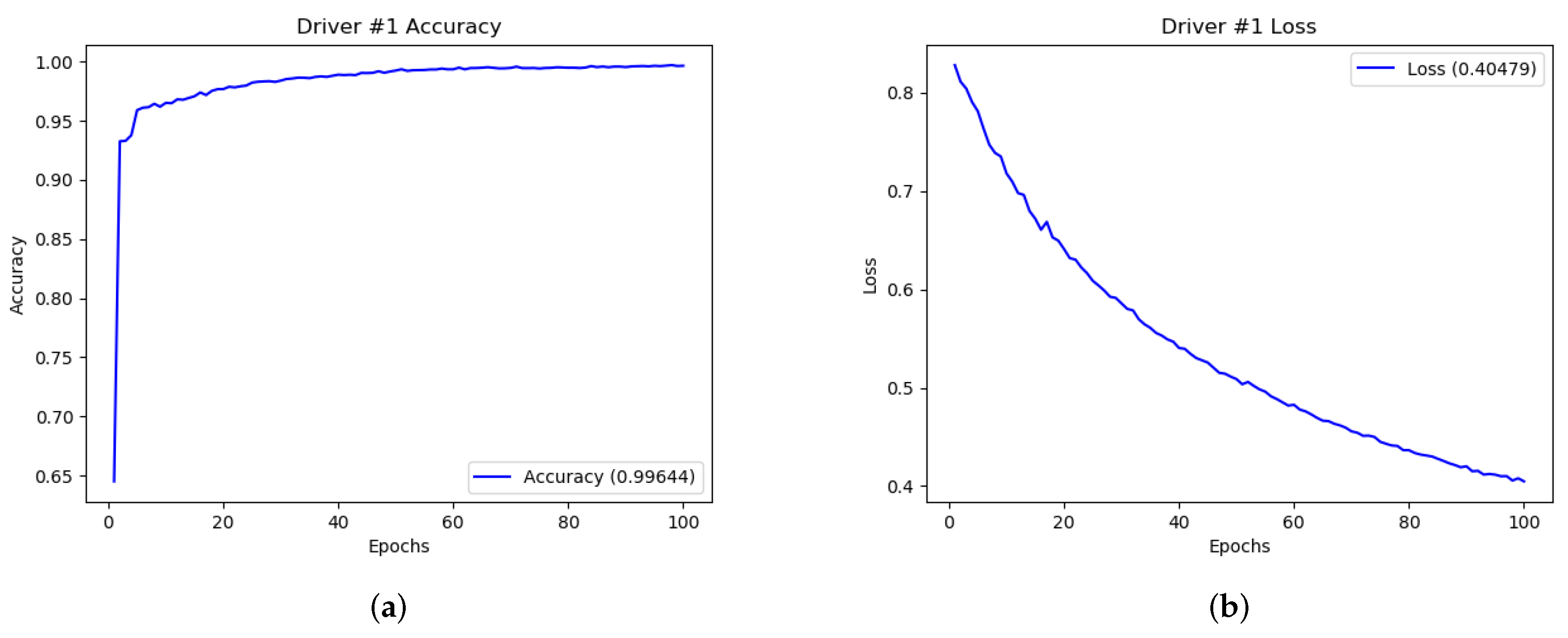
From the Accuracy and Loss definitions, it is expected that Accuracy and Loss should be inversely proportional—for high values of accuracy, low loss values are expected (and the opposite). Furthermore, considering that the weights and bias are initially random selected, the accuracy trend should start by exhibiting low values (and high loss value, symptomatic that the network is performing wrong predictions), but whether the network during the several “epochs” (i.e., one forward pass and one backward pass of all the training examples) is able to learn (i.e., it is able to solve the driver prediction problem), the accuracy should start to exhibit higher values in the next iterations (and consequently the loss should exhibit low values). The epoch is a parameter chosen by the network designer, usually the number of epochs chosen is such that the loss is at least and it does not get worse in the immediately succeeding epochs and, consequently, the accuracy value reached is the maximum and in the immediately succeeding epochs is not improving, symptomatic that the network has reached the stability and that further epochs would not improve performances. We set the number of epochs equal to 100, because the three networks reached the stability with a number less or equal to 100.

Figure 9 shows the performances (in terms of accuracy and loss) related to Driver #1 detection. We only show some accuracy and loss plots, considering that the remaining plots are similar to the ones shown.

With regard to the effectiveness of the proposed neural learning network in driver detection we obtain that the average accuracy is equal to 0.99 and the average loss is equal to 0.40.

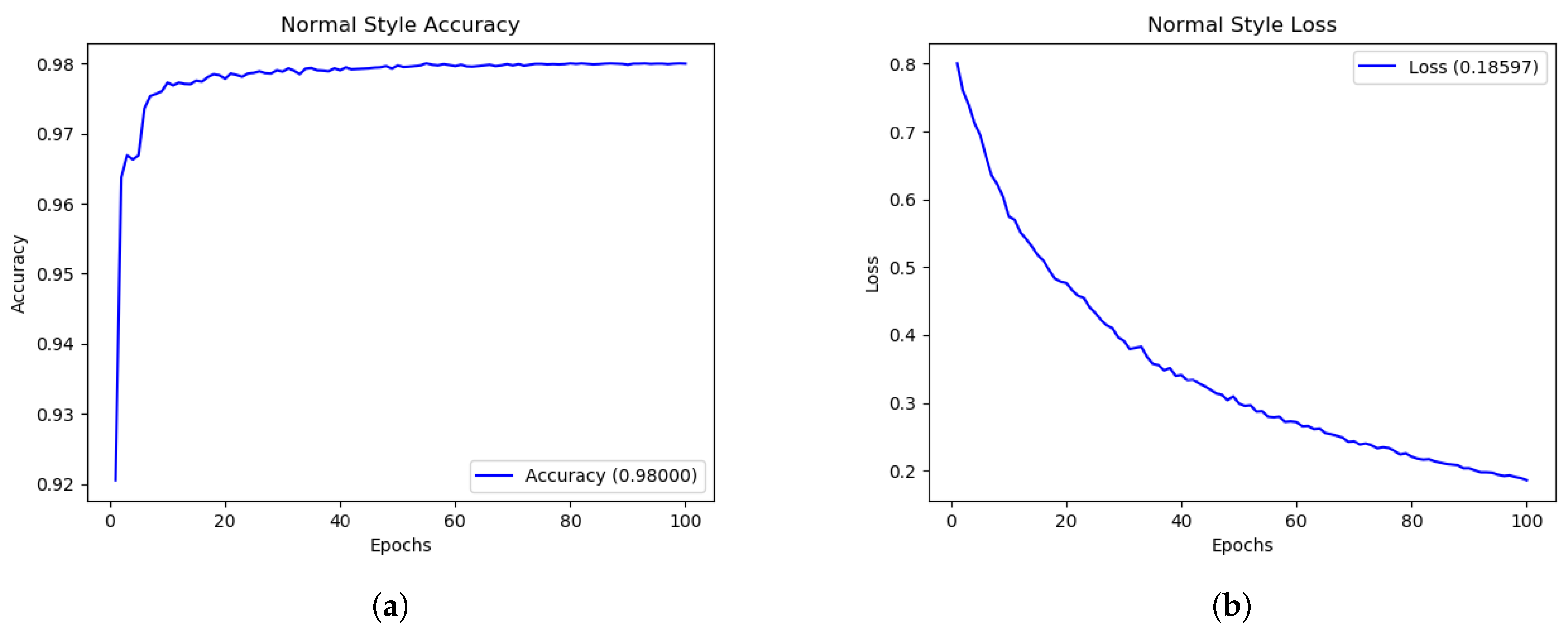
Figure 10 shows the performances (in terms of accuracy and loss) related for driving style detection.

Following results are obtained: with regard to the Normal Style an accuracy equal to 0.98 and a loss of 0.18 is obtained while, for the Drowsy Style detection an accuracy of 0.92 and a loss of 0.28 is reached and, finally, relating to the Aggressive Style detection an accuracy of 0.98 and a loss of 0.017 is obtained.

In Figure 11 are depicted the performances (in terms of accuracy and loss) related to secondary road identification.

With regard to road detection, the neural network architecture we designed following results are reached: for the Secondary Road detection an accuracy equal to 0.96 and a loss equal to 0.10 is obtained while, relating to the Motorway Road detection an accuracy of 0.91 and a loss equal to 0.26.

5. Related Work

Current literature related to the driver behavioural analysis in discussed in following section.

Features from accelerator and the steering wheel were analyzed by researchers in [20]. Observing these characteristics, they exploit hidden Markov model (HMM) to model drivers. They basically consider two different models for each driver under analysis, the first model is trained from accelerator features while the second model is trained from steering wheel features. The models can be used to identify different drivers with an accuracy equal to 85%.

Researchers in [21] classify a set of features extracted from the power-train signals of the vehicle, showing that their classifier is able to classify the human driving style based on the power demands placed on the vehicle power-train with an overall accuracy equal to 77%.

In order to study driver behavior questionnaire and self-reports have been explored [22] questionnaires provide a means for studying driving behaviors, which could be difficult or even impossible to study by using other methods like observations, interviews and analyses of national accident statistics. Their findings demonstrate that that bias caused by socially desirable responding is relatively small in driver behavior questionnaire responses.

Van Ly et al. [23] explore the possibility of using the inertial sensors of the vehicle from the CAN bus to build a profile of the driver observing braking and turning events to characterize an individual compared to acceleration events.

Researchers in [24] model gas and brake pedal operation patterns with Gaussian mixture model (GMM). They achieve an identification rate equal to 89.6% for a driving simulator and 76.8% for a field test with 276 drivers, resulting in 61% and 55% error reduction, respectively, over a driver model based on raw pedal operation signals without spectral analysis.

Authors in [25] design a driver identification method that is based on the driving behavior signals that are observed while the driver is following another vehicle. They analyzed signals, as accelerator pedal, brake pedal, vehicle velocity, and distance from the vehicle in front, were measured using a driving simulator. The identification rates were 81% for twelve drivers using a driving simulator and 73% for thirty drivers.

Driver behavior is described and modeled in [26] using data from steering wheel angle, brake status, acceleration status, and vehicle speed through Hidden Markov Models (HMMs) and GMMs employed to capture the sequence of driving characteristics acquired from the CAN bus information. They obtain 69% accuracy for action classification, and 25% accuracy for driver identification.

In reference [27] the features extracted from the accelerator and brake pedal pressure are used as inputs to a Fuzzy Neural Network (FNN) system to ascertain the identity of the driver. Two fuzzy neural networks are designed by authors to show the effectiveness of the two proposed feature extraction techniques.

Authors in [28] propose a method based on driving pattern of the car. They consider mechanical feature from the CAN vehicle evaluating them with four different classification algorithms, obtaining an accuracy equal to 0.939 with Decision Tree, equal to 0.844 with k Nearest Neighbor (KNN), equal to 0.961 with RandomForest and equal to 0.747 using Multilayer Perceptron (MLP) algorithm.

A hidden-Markov-model-(HMM)-based similarity measure is proposed in [29] in order to model driver human behavior. They employ a simulated driving environment to test the effectiveness of the proposed solution.

Nor and colleagues [30] adopt a set of features to recognize the emotion of the driver by using multi layer perceptron (MLP) as classifiers. The data collection was conducted in Singapore. The driver must have at least two years driving experience. They managed to collect 11 drivers including men and women, aged between 24–25 years old. The considered features are the brake and gas pedal pressures. In the experiment they state that each driver meets the accuracy level which is more than 50%: the highest accuracy is obtained from driver 10 with an accuracy equal to 71.94%, while the lowest accuracy is obtained from driver 3 with an accuracy equal to 61.65% in classification according to the other driver.

Authors in [31,32] propose a method to detect aggressive drivers. They design a scoring by employing fuzzy logic by adopting smartphone accelerometers and GPS. In order to evaluate the proposed mechanism, they collected traces from twenty vehicles equipped with an Android application developed by authors.

Castignani et alius [33,34] discuss SenseFleet, a driver profile platform that is able to detect risky driving events independently from the mobile device and vehicle. They use a Fuzzy system to compute a score for the different drivers using real-time context information like route topology or weather conditions. The method is evaluated considering multiple drivers along a predefined path, showing that SenseFleet is able to detect risky driving events and provide a representative score for each individual driver.

Researchers in [35], to control the road and driver behavior, propose a metric to measure the casualty crash for assessing the effectiveness of a PAYD (i.e., pay-as-you drive) scheme. They show that in several cases personalized feedback alone is sufficient to induce significant changes, but the largest reductions in risk are observed when drivers are also awarded a financial incentive to change behavior.

A biometric driver recognition system utilizing driving behaviors is proposed in [35]. The authors, using Gaussian mixture models, extracted a set of features from the accelerator and brake pedal pressure was then used as inputs to a fuzzy neural network system to ascertain the identity of the driver. Their experiment shows the effectiveness of the use of the FNN for real-time driver identification and verification.

Jazayeri et alius [36] consider the video analysis to detect and track vehicles. They basically propose an approach with the aim to localize target vehicles in video under different environmental conditions. They train an hidden Markov Model to discern target vehicles from the background in order to track them.

Miyajima et al. [37] propose a set of characteristics gathered by exploiting spectral analysis from driving sessions building a model through a GMM. Authors obtained their evaluated dataset with both a driving simulator and a real car. Experimental results show that this approach reaches a detection rate equal to 89.6% for driving simulator and 76.8% for real vehicle.

Trasarti et alius [38] extract mobility profiles of individuals from raw GPS traces studying how to match individuals based on profiles. They instantiate the profile matching problem to a specific application context, namely proactive car pooling services, and therefore develop a matching criterion that satisfies various basic constraints obtained from the background knowledge of the application domain.

Petzoldt and colleagues [39] analyze the influence on accident involvement of younger drivers. They develop a Computer based training module to complement existing driver training programs by addressing critical cognitive skills. The developed module employs video sequences of potentially hazardous driving situations, including multiple-choice questions with adaptive feedback, in order to increase levels of elaboration and understanding. Authors concluded that Computer based training can potentially assist instruction of cognitive skills necessary for save driving.

Wu et al. [40] presents a study related to driver’s voice feature selection and classification for speaker identification in vehicle systems. The designed system consists of a combination of feature extraction using continuous wavelet technique and voice classification using artificial neural network. In the feature extraction, a time-averaged wavelet spectrum based on continuous wavelet transform is proposed. Meanwhile, the artificial neural network techniques were used for classification in the proposed system. To verify the proposed system, they consider a conventional back-propagation neural network (BPNN) and generalized regression neural network (GRNN)—the experimental results obtain an identification rate equal to 92% for using BPNN and 97% for using GRNN approach.

The authors of [41] consider the identification of distracted drivers rather than focus on the driver identification. They analyse three CAN-Bus signals (i.e., vehicle speed, steering wheel angle and brake force) and three different maneuvers (left turn, right turn and lane change). In addition, as features, the authors also consider the driver and the road videos, the driver speech, the distance sensor using laser, the GPS sensor for position measurement. Their method basically adopts HMM to discover the optimum number of states for each maneuver. The driving scenarios include two different routes—residential and commercial areas, while each route is driven by each driver twice—neutral and distracted.

Carfora and colleagues [8] design an approach aimed to detect the driver driving style by considering the adoption of unsupervised machine learning techniques. They evaluate the proposed method with a real-world case study. Moreover, they discuss how the proposed method can be considered as risk indicator for car insurance companies.

Martinelli et al. [42] consider the task of driver aggressiveness detection by exploiting unsupervised classification techniques. They design a model with a set of features from the CAN bus of a real-world vehicle while traveling in urban and highway roads.

Researchers in [9] starting from a set of features gathered from the in-vehicle CAN bus, exploit several machine learning algorithms to distinguish between the car owner and impostors. Moreover, they assess the proposed machine learning models effectiveness in the evaluation of instances not evaluated in the training set.

Researchers in [19] collected a set of numerical features for driver identification and path detection. They consider supervised machine learning, in detail they exploit a time-series classification approach based on a multilayer perceptron (MLP) network.

The authors of [43] proposed the adoption of the MLP network to build a model based on feature obtained from the CAN bus for the driver detection task, considering in the experimental analysis 10 different drivers.

The author of [44] proposed a method to automatically detect driver distraction. They consider a convolutional neural network for detecting behaviours as, drinking or adjusting radio, by analysing video streams. They obtain an average accuracy equal to 0.80.

Zhang et al. [45] proposed a driver distraction method by exploiting a deep learning (DL) approach. Their approach is related to the adoption of three main modules: multi-modal representation learning, multi-scale feature fusion and unsupervised driver distraction detection, obtaining an accuracy equal to 0.97.

Researchers in [46] exploit a convolutional neural network for distracted driver detection. They consider transfer learning, using the VGG16 pretrained model, obtaining an accuracy of 0.96.

The authors of [47] adopt a convolutional neural network for the extraction of the representation of eye and mouth fatigue from the face area detected from video frame. Their driver drowsiness detection method obtains an accuracy equal to 0.75.

Yun et al. [48] developed a clustering-based method to transform various vehicle data into cluster coordinates, to analyze data distribution, to analyze sampled cluster data and decide cluster characteristics, and to predict and monitor vehicle abnormal states. Differently from our proposal, this is work is related to safety.

Table 4. Current Literature Comparison on Driver Behaviour Classification (column Research) expressed in terms of: publication year (column Year), dataset source (column Dataset) real data extracted from the Controller Area Network (CAN) bus (i.e., CAN) or using a software simulator (i.e., Driver simulator) and other data obtained by software systems, the algorithms involved in the classification task (column Algorithm) and the considered task (Driver Detection (column DD, Driving Style (column DS and Road Detection (column RD).

Research	Year	Dataset Based on	Algorithm	DD	DS	RD
Wakita et al. [25]	2006	Driver Simulator	MLP, FNN	✓
Zhang et al. [20]	2014	Driver Simulator	HMM	✓
Kedar-Dongarkar et al. [21]	2012	CAN	KNN, HMM	✓
Van Ly et al. [23]	2013	CAN	K-means, SVM	✓
Miyajima et al. [24]	2007	Driver simulator, CAN	GMM	✓
Nishiwaki et al. [49]	2007	CAN	GMM	✓
Choi et al. [26]	2007	CAN	HMM	✓
Wahab et al. [50]	2009	Vehicle sensor data, video streams, voice streams	GMM, FNN, MLP	✓
Meng et al. [27]	2006	Driver simulator	HMM	✓
Bernardi et al. [43]	2018	CAN	MLP	✓
Enev et al. [29]	2016	CAN	SVM, RandomForest, Naïve Bayes, KNN	✓
Kwak et al. [28]	2016	CAN	Decision Tree, KNN, RandomForest, MLP	✓
Bernardi et al. [19]	2018	CAN	MLP	✓		✓
Miyajima et al. [37]	2006	Driver Simulator, CAN	GMM	✓
Nor et al. [30]	2010	CAN	MLP	✓
Martinelli et al. [10]	2018	CAN	J48	✓
Carfora et al. [8]	2019	CAN	k-means		✓
Martinelli et al. [42]	2018	CAN	k-means		✓
Martinelli et al. [9]	2020	CAN	SVM, RandomForest, J48	✓
Chen et al. [44]	2020	video streams	CNN		✓
Zhang et al. [45]	2020	video streams	CNN		✓
Narayanan et al. [46]	2021	video streams	CNN		✓
Chen et al. [47]	2021	video streams	CNN		✓
Our Approach	2021	feature obtained from mobile device/ info-entertainment system	CNN	✓	✓	✓

presents a comparison of the proposed approach with respect to the current state-of-the-art literature.

In

Table 5. Current Literature Comparison on Driver Detection (column Research) expressed in terms of: features considered (column Features) and the obtained performances (column Detection Rate).

Research	Features	Detection Rate
Wakita et al. [25]	accelerator pedal, brake pedal, vehicle velocity, distance from the vehicle in front	73%
Zhang et al. [20]	accelerator, steering wheel	85%
Kedar-Dongarkar et al. [21]	vehicle acceleration, braking, speeding index, throttle activity	77%
Van Ly et al. [23]	accelerator, braking, turning	65%
Miyajima et al. [24]	distance, velocity, gas pedal, brake pedal	89.6%
Nishiwaki et al. [49]	gas pedal, brake pedal	76.8%
Choi et al. [26]	steering wheel angle, brake status, acceleration status, speed	70%
Wahab et al. [50]	accelerator pedal, brake pedal	95%
Meng et al. [27]	acceleration, brake, steering wheel	80%
Bernardi et al. [43]	CO${}_2$ consumption computed in average, Instantaneous cost for kilometer, Trip cost for kilometer, Percentage load of the engine, Engine RPM, GPS Speed, Liters Per 100 Kilometer (Instant) (L/100 km)	95%
Enev et al. [29]	brake pedal position, steering wheel angle, lateral acceleration, yaw rate, gear shift lever, speed, estimated gear, shaft angular velocity, accelerator pedal, engine speed (RPMs), driver requested torque, maximum engine torque, fuel consumption rate, throttle position, turn signal	100%
Kwak et al. [28]	long term fuel trim, intake air pressure, accelerator pedal value, fuel consumption, friction torque, maximum indicated engine torque, engine torque, calculated load value, activation of air compressor, engine coolant temperature, transmission oil temperature, wheel velocity front left-hand, wheel velocity front right-hand, wheel velocity rear left-hand, torque converter speed	93%
Bernardi et al. [19]	CO${}_2$ consumption computed in average, Instantaneous cost for kilometer, Trip cost for kilometer, Percentage load of the engine, Engine RPM, GPS Speed, Liters Per 100 Kilometer (Instant) (l/100 km)	96%
Miyajima et al. [37]	pedal pressure, brake pedal pressure, and steering angle, velocity, acceleration, engine speed	89.6%
Nor et al. [30]	brake and gas pedal pressures	71.94%
Martinelli et al. [10]	intake air pressure, engine soacking time, long term fuel trim bank1, torque of friction, transmission oil temperature, steering wheel speed	98%
Martinelli et al.	intake air pressure, engine soacking time, long term fuel trim bank1, torque of friction, trasmission oil temperature, steering wheel speed	99%
Martinelli et al. [9]	Intake air pressure, torque of friction	0.93
Our Approach	Acceleration, roll, pitch, yaw	0.99

, we propose an overview related to the driver detection task (as highlighted in this section, the one most considered by researchers). We compare the state-of-the-art work in terms of features exploited and the detection rate obtained.

As shown from the driver detection results shown in Table 5 the only work obtaining a high detection rate by exploiting features not obtained from the CAN bus is the one we propose. Nonetheless, there are several work in literature obtaining high performances (i.e., references [10,29] but these methods require the permanent connection to the CAN bus of vehicle under analysis.

The main difference with regard to the elicited works is that, in this paper, we propose an architecture aimed to identify the driver, the driving style and the kind of road travelled exploiting feature related to the accelerometer sensor available from the info-entertainment system or in a mobile device fixed in the vehicle. In fact, each cited work is focused only on the driver detection or on the driving style detection, moreover several works considered a simulated environment and not the real one (and these ones require to access to sensitive information transiting on the CAN bus). This represents the first attempt to detect the driver, the driving style and the road exploiting the same feature set, overcoming the state of the art literature in terms of performances.

6. Conclusions and Future Work

In this paper we presented a neural network architecture aimed to provide a framework to analyse driver behaviours aimed to detect (i) the driver, (ii) the driving style and (iii) the travelled road.

We evaluated the proposed method by exploiting two real-world datasets composed by a total of 16 different drivers obtaining the analysed feature vector from the accelerometer integrated into a fixed mobile device (i.e., a smartphone). We obtained an accuracy equal to 0.99 for the driver identification, an accuracy ranging from 0.92 and 0.98 related to style detection and an accuracy ranging to 0.91 to 0.96 for road identification.

With regard to the limitations of the proposed method, one of the most recently discussed problems that afflicts deep learning techniques and artificial intelligence in general, is the lack of explainability and interpretability of the results. In fact, researchers in the field of artificial intelligence are recently proposing solutions that can explain the predictions obtained from a model. We will consider to integrate in the proposed method a way to provide the visual explanations [51,52] of the results, as already provided in other contexts for instance, in the COVID-19 detection [53].

As future work, we plan to investigate whether the application of formal methods [54,55,56] can be useful for the driver, driving style and road identification, which have been already successfully used in other domains like, for instance, malware detection [57,58,59] and in system biology [60].