Application of Gaussian Radial Basis Functions for Fast Spatial Imaging of Ground Penetration Radar Data Obtained on an Irregular Grid

Abstract

Spatial imaging of ground penetrating radar (GPR) measurement data is a difficult computational problem that is time consuming and requires substantial memory resources. The complexity of the problem increases when the measurements are performed on an irregular grid. Such grid irregularities are typical for handheld or flying GPR systems. In this paper, a fast and efficient method of GPR data imaging based on radial basis functions is described. A compactly supported modified Gaussian radial basis function (RBF) and a hierarchical approximation method were used for computation. The approximation was performed in multiple layers with decreasing approximation radius, where in successive layers, increasingly finer details of the imaging were exposed. The proposed method provides high flexibility and accuracy of approximation with a computational cost of N·log (N) for model building and N·M for function evaluation, where N is the number of measurement points and M is the number of approximation centres. The method also allows for the control smoothing of measurement noise. The computation of one high-quality imaging using 5000 measurement points utilises about 5 s on an Intel Core i5-7200U CPU 2.5 GHz, 8 GB RAM computer. Such short time enables real-time image processing during field measurements.

1. Introduction

Ground penetrating radars (GPRs) are electromagnetic systems for soil subsurface structure imaging. To obtain imaging that is precise enough for correct interpretation beside of specific electrical system the respectively accurate positioning, data must be registered. Software that is commonly used for processing the obtained data set commonly assumes that the measurements were made on a simple rectangular grid. The GPR operators usually try to fulfil such requirements to obtain the best possible imaging using the software.

Unfortunately, there are many situations where the requirements cannot be fulfilled. Typical situations take place in handheld systems where measurement points are located randomly toward a curved trajectory. In general, the problem concerns all scanning echolocation systems where spatial distribution of measurement points is random but dense enough. A separate issue is the accurate positioning method.

When the measurements cannot be made on a simple rectangular grid due to handheld operation or inaccessibility of some locations, as a result the data from irregularly located measurement points are registered. Meshless approximation methods should then be used for spatial imaging. At present, a variety of meshless methods are used in geosciences for digital terrain model generation, such an inverse distance weighting (IDW) [1,2], triangulated irregular network (TIN) with linear interpolation [3,4], natural neighbour (NN) [5,6] radial basis functions (RBFs) [7] and kriging [8]. The implementation of these algorithms can be found many different applications e.g., Ref. [9]. They can now be found on geophysical packages, such as Surfer [10], Geosoft Oasis Montaj Geoscience [11] and TerrSet [12]. However, all of the packages are geared towards solving slightly different physical problems than GPR data analysis. First, with typical geophysical surveys, there are relatively equidistant points, except for some local areas. In the case of handheld GPR, there are densely distributed points along the curved scanning path, and the distances between successive paths are very large compared to the distances between successive survey points. This causes problems with setting up a computational mesh and ill-conditioning of many classical methods. Another problem arises from the large amount of measurement data. A single point measurement generates hundreds of numbers corresponding to echo values coming from different depths. This requires data pre-processing to prepare the input data for geophysical packages. All this makes the available computational packages, which are valuable for the final analysis of the results, unable to fulfil their role during field measurements, where real-time processing and simplicity of use are required.

A method to get around this problem is to create custom software. All methods of interpolation and approximation of multidimensional data boil down to solving systems of matrix equations. Due to the complexity of computational procedures, ready-made libraries of numerical procedures, which contain optimised implementations of solvers for linear algebraic equation systems, are extremely helpful. One such package is ALGLIB [13], which also has procedures for interpolation and approximation of multidimensional data.

This paper presents a method of visualising spatial GPR data using RBFs. A modified Gaussian function was used as the RBF, so that it assumed a value of zero at the given distance from the centre. This method provides ease of use, flexibility and high interpolation accuracy. It also allows for the suppression of measurement noise.

2. Radial Basis Functions (RBFs)

A radial basis functions (RBFs), $\varphi$, is a function whose value depends only on the distance from the origin or some other fixed point, c, called a centre, so that $\varphi \left(x\right)=\varphi \left(\Vert x-c\Vert \right)$. The distance, $r=\Vert x-c\Vert$, is usually Euclidean; although, other metrics are sometimes used. Since the average distance between points can vary greatly depending on the problem being studied, it is convenient to use the concept of the RBF radius, R₀. It is the shape parameter that defines the behaviour of the function. Using the radius, the scaled distance can be defined as $r_s=r/R_0$ and used to calculate RBFs.

There are two main groups of basis functions: global RBFs and compactly supported RBFs (CS-RBFs) [14]. Global RBFs have non-zero values at any distance from the centre; although, some of them can drop quickly with distance. CS-RBFs are positive only within a certain radius from the centre and are zero outside of it.

Scattered data adjusting with CS-RBFs caused faster and simpler calculation as a linear equations system has a sparse matrix. Nevertheless, approximation using CS-RBFs is susceptible to the density of the approximated scattered data and to the selection of shape parameter. Typical examples of local RBFs are shown in

Table 1. Examples of compactly supported RBFs; “+” means value zero out of the scaled distance <0, 1> [15].

ID	Function	ID	Function
1	${\left(1-r_s\right)}_{+}$	6	${\left(1-r_s\right)}_{+}^6\left(35r_s{}^2+18r_s+3\right)$
2	${\left(1-r_s\right)}_{+}^3\left(3r_s-1\right)$	7	${\left(1-r_s\right)}_{+}^8\left(32r_s{}^3+25r_s{}^2+8r_s+1\right)$
3	${\left(1-r_s\right)}_{+}^5\left(8r_s{}^2-5r_s+1\right)$	8	${\left(1-r_s\right)}_{+}^3$
4	${\left(1-r_s\right)}_{+}^2$	9	${\left(1-r_s\right)}_{+}^3\left(5r_s+1\right)$
5	${\left(1-r_s\right)}_{+}^4\left(4r_s+1\right)$	10	${\left(1-r_s\right)}_{+}^7\left(16r_s{}^2+7r_s+1\right)$

.

Typical global RBFs are Gauss, $\exp \left(-r_s^2\right)$, inverse quadratic, ${\left(1+r_s^2\right)}^{-1}$, and inverse multiquadric, ${\left(1+r_s^2\right)}^{-1/2}$. Along with increasing radius, r, RBFs are monotonically decreases, strictly positive definite, infinitely differentiable and convergent to zero. Another globally well-known RBFs is thin plate spline (TPS), $r^{2k}\ln \left(r\right)$, $k\in N$, without shape parameter and which is disparate while increasing radius. TPS has a singularity at the origin, which is removable for the function, and its first derivative but this singularity is not removable for the second derivative of TPS [16]. In the case of a great number of points, global RBFs cause an ill-conditioned linear system of equations (LSE) with a dense matrix, which can lead to convergence problems.

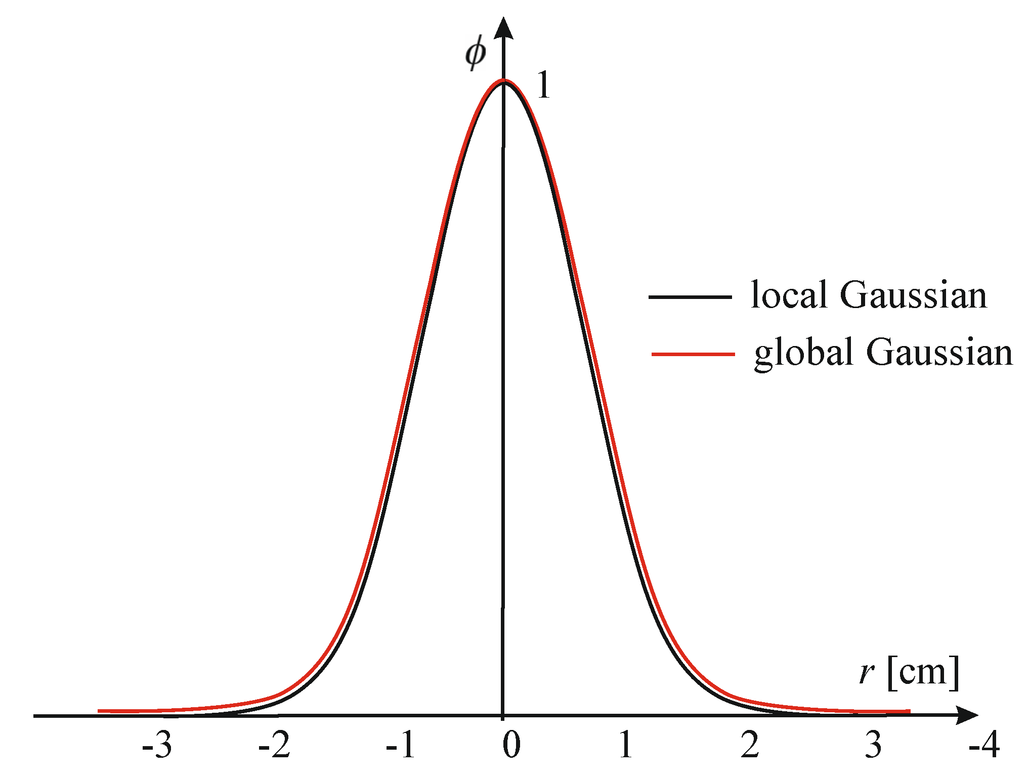
The ALGLIB package implements both kinds of RBFs: the global Gaussian function and compactly supported. The classical Gaussian function takes small values already at a distance of about 3R₀ from the center and can easily be modified to be compactly supported. ALGLIB implementation of such function is expressed by the following exponential form:

$$\exp \left(1-\frac{r^2}{R_0^2}-\frac{1}{1-r^2/{\left(3R_0\right)}^2}\right)$$

(1)

RBF (1) differs little in shape from the Gaussian function while having all the advantages of a compactly supported function. It reaches zero at a distance of R₀ = 3. The shapes of both functions are shown in Figure 1.

Radial basis functions can be used to process scattered data from GPR. Two types of approaches are used for this purpose: RBF interpolation or approximation.

3. RBF Interpolation

In the interpolation process, we are looking for a function $f\left(x\right)$ that at N measuring points $x={\left\{\mathit{x}\right\}}_1^N$, $\mathit{x}={\left(x_1,x_2\right)}^{\mathrm{T}}$ obtains the same values as the measured $h={\left\{h\right\}}_1^N$. RBF interpolation is based on determining the distance of two points (in the d-dimensional space in general) and is provided by the following form:

$$f\left(x\right)={\displaystyle \sum _{j=1}^N{w}_j\varphi \left(\Vert x-{\mathit{x}}_j\Vert \right)}$$

(2)

where the interpolating function $f\left(x\right)$ is represented as a sum of N RBFs, each centered at a different data point, ${\mathit{x}}_j$, and weighted by an appropriate coefficient, $w_j$. For the given dataset, this leads to an LSE, as follows:

$$f\left({\mathit{x}}_i\right)={\displaystyle \sum _{j=1}^N{w}_j\varphi \left(\Vert {\mathit{x}}_i-{\mathit{x}}_j\Vert \right)}$$

(3)

which can be represented in matrix form as the following:

$$Aw=h$$

(4)

where $A=\left\{A_{i,j}\right\}=\left\{\varphi \left({\mathit{x}}_i-{\mathit{x}}_j\right)\right\}$ is the N × N symmetric matrix, the vector $w={\left(w_1,w_2,\dots ,w_N\right)}^T$ is the vector of unknown weights, and $h={\left(h_1,h_2,\dots ,h_N\right)}^T$ is the vector of values in the given points. After solving the system of linear equations, the interpolated value at point $\mathit{x}$ is computed using Equation (2). The disadvantage of RBF interpolation is the large and usually ill-conditioned design matrix of the LSE.

The calculation of the coefficients, w, for all measuring points (interpolation) is, in many cases, computationally expensive. However, for good-quality spatial imaging, it is often enough to have a much smaller number of coefficients, especially if the measurements are made densely. Then, the computed function, f (x), does not take exactly experimental values, but the errors may be so small that they can be completely accepted. This approach is called the RBF approximation [17].

The simplest approach to solving the approximation problem is the least square method (LSM). We consider a modified interpolation formula, as follows:

$$f\left(x\right)={\displaystyle \sum _{j=1}^M{w}_j\varphi \left(\Vert x-c_j\Vert \right)}$$

(5)

where $c_j$ is not the measuring point but the reference point of the grid on which we want to perform the calculations. The mesh contains M nodes and may be irregular in general; although, computationally convenient rectangular meshes are usually used. The number of nodes can be many times smaller than the number of measurement points (M << N), which speeds up the calculations accordingly.

For the dataset, Equation (5) gives an overdetermined LSE, as follows:

$$f\left({\mathit{x}}_i\right)={\displaystyle \sum _{j=1}^M{w}_j\varphi \left(\Vert {\mathit{x}}_i-{\mathit{c}}_j\Vert \right)} i=1,\dots ,N$$

(6)

The linear system of Equation (6) can be represented as the matrix Equation (4). In the expanded form:

$$\left[\begin{array}{ccc}{\varphi }_{1,1}& \cdots & {\varphi }_{1,M}\\ ⋮& \ddots & ⋮\\ {\varphi }_{i,1}& \cdots & {\varphi }_{i,M}\\ ⋮& \ddots & ⋮\\ {\varphi }_{N,1}& \cdots & {\varphi }_{N,M}\end{array}\right]\left[\begin{array}{c}{w}_1\\ ⋮\\ w_M\end{array}\right]=\left[\begin{array}{c}{h}_1\\ ⋮\\ h_i\\ ⋮\\ h_M\end{array}\right]$$

(7)

This LSE can be solved by the LSM as $A^{\mathrm{T}}Aw=A^{\mathrm{T}}h$, singular value decomposition, etc. Reducing the number of points speeds up the $w$ computation by a factor of O((M/N)³) as the LSE computational is of O(M³) [18].

This method can have problems with stability and solvability. Therefore, the RBF approximant (5) is usually extended by the polynomial function $P_k\left(x\right)$ of degree k, as follows:

$$f\left(x\right)={\displaystyle \sum _{j=1}^M{w}_j\varphi \left(\Vert x-{\mathit{x}}_j\Vert \right)}+P_k\left(x\right)$$

(8)

In practice, a linear polynomial is the following, or a constant term is used:

$$f\left(x\right)={\displaystyle \sum _{j=1}^M{w}_j\varphi \left(\Vert x-{\mathit{x}}_j\Vert \right)}+P_k\left(x\right)$$

(9)

For the linear term, the matrix equation can be rewritten as the following:

$$\left[\begin{array}{cccccc}{\varphi }_{1,1}& \cdots & {\varphi }_{1,M}& x_1& y_1& 1\\ ⋮& \ddots & ⋮& ⋮& ⋮& 1\\ {\varphi }_{i,1}& \cdots & {\varphi }_{i,M}& x_i& y_i& 1\\ ⋮& \ddots & ⋮& ⋮& ⋮& 1\\ {\varphi }_{N,1}& \cdots & {\varphi }_{N,M}& x_N& y_N& 1\end{array}\right]\left[\begin{array}{c}{w}_1\\ ⋮\\ w_M\\ a_x\\ a_y\\ a_0\end{array}\right]=\left[\begin{array}{c}{h}_1\\ ⋮\\ h_i\\ ⋮\\ h_N\end{array}\right]$$

(10)

For two-dimensional space, a linear system of N equations in M + 3 variables must be solved, where N is the number of points in the given dataset and M is the number of references. Such system is overdetermined again and can also be solved by the same methods. If global RBFs are used, matrix A is dense, while in the case of CS-RBF this matrix can be sparse.

If LSE is solved directly, the matrix equation A^TAw = A^Th must be solved. The $A^{\mathrm{T}}A$ matrix is ill-conditioned, and for large M the system of linear equations is difficult to solve [19]. Moreover, the matrix size is 2M × 2M. This means that the memory requirements are not acceptable even for medium data sets. For real applications of the RBF approximation, we need to decrease memory requirements significantly. There are various approaches to solving these problems, the most important of which are listed below.

4. Model Construction

After selecting the basis function (and optionally the polynomial term), we calculate the weight coefficients, and thereby can build the model. There are several ways to approach the issue. Certain functions can be used for both global and compact basis functions [13]:

• “Straightforward” approach: using a dense solver to the linear system. Performs with any basis function, but it has low efficiency as the solution time increases with the number of points, N, as O(N³). Thus, this approach is limited to several thousand points.
• Preconditioning: preconditioning approximate cardinal basis function (ACBF) to accelerate convergence [20]. In this case, several non-local basis functions are constructed to build another local basis function (cardinal basis function). Usually, the solution itself only requires some of the total processing time, and most of it is spent on the construction of the new basis. In dense systems that we obtain with global basis functions, preconditioning allows for good performance with iterative solver to be achieved. In the case of CS-RBFs, compact functions become “more compact,” which allows us to use iterative solvers with quite a large radius, equal to two distances to the nearest neighbour.

Regarding compact basis functions, it is possible to use a sparse linear solver, both iterative or direct. Convergence of the iterative solver depends on system conditioning, what easily solve problems with a small radius (approximately equal to the distance to the nearest neighbour), but it will have difficulties with larger one. From the different side, it does not need additional memory. Problems with larger radii (up to 2–3 distances) can be solve by direct solver but it requires more memory to store Cholesky or LU apportionment of the system.

Dividing the original dataset into few smaller ones [21] is the next method used with compact functions, which allows for the problem of RBF construction to be tackled apart for above mentioned smaller parts, and next, the fractional model is put together into a larger, global one. However, composition of the model is imperfect, and the artifacts are nearly to the boundaries what causes that the problem with interpolation have to be tackled anew to correct the errors of the first model. As an outcome, we obtain iterative algorithms, which repeat the “separate-solve-compose-correct” loop several times before achieving the desirable accuracy.

The above described algorithms have one common attribute: they solve the original problem without any modifications. Nevertheless, by changing the problem characteristic slightly we can receive a good interpolant with repeatedly greater efficiency. For instance, we can use more functions with different radii, instead of N Gaussian functions with the same radii. The approximation difficulty can be tackled in a few steps by building a hierarchy of a precise model with decreasing radii. Such an approach has different terms: multiscale RBF, multilevel RBF, hierarchical RBF or multilayer RBF (RBF-ML). Its main asset is high efficiency and precision due to the hierarchy of easy to build application.

5. RBF-ML Interpolation Algorithm

In this paper, the RBF-ML algorithm implemented in the ALGLIB package was used. It has three parameters: the initial radius, R₀, the number of layers, N_L, and the regularisation coefficient, λ. This algorithm builds a hierarchy of models with decreasing radii [13].

In the initial (optional) iteration, the algorithm builds a linear least squares model. The values predicted by the linear model are subtracted from the function values at the nodes, and the residual vector is passed to the next iteration. In the first iteration, a traditional RBF model with a radius equal to R₀ is built. However, it does not use a dense solver and does not try to solve the problem exactly. It solves the least squares problem by performing a fixed number (approximately 50) of LSQR [22] iterations. Usually, the first iteration is sufficient. Additional iterations will not improve the situation because with such a large radius, the linear system is ill-conditioned. The values predicted by the first layer of the RBF model are subtracted from the function values at the nodes, and, again, the residual vector is passed to the next iteration. With each successive iteration, the radius is halved by performing the same constant number of LSQR iterations, and the forecasts of the new models are subtracted from the residual vector.

In all subsequent iterations, a fine regularisation can be applied to improve the convergence of the LSQR solver. Larger values for the regularisation factor can help reduce data noise. Another way of controlled smoothing is to select the appropriate number of layers.

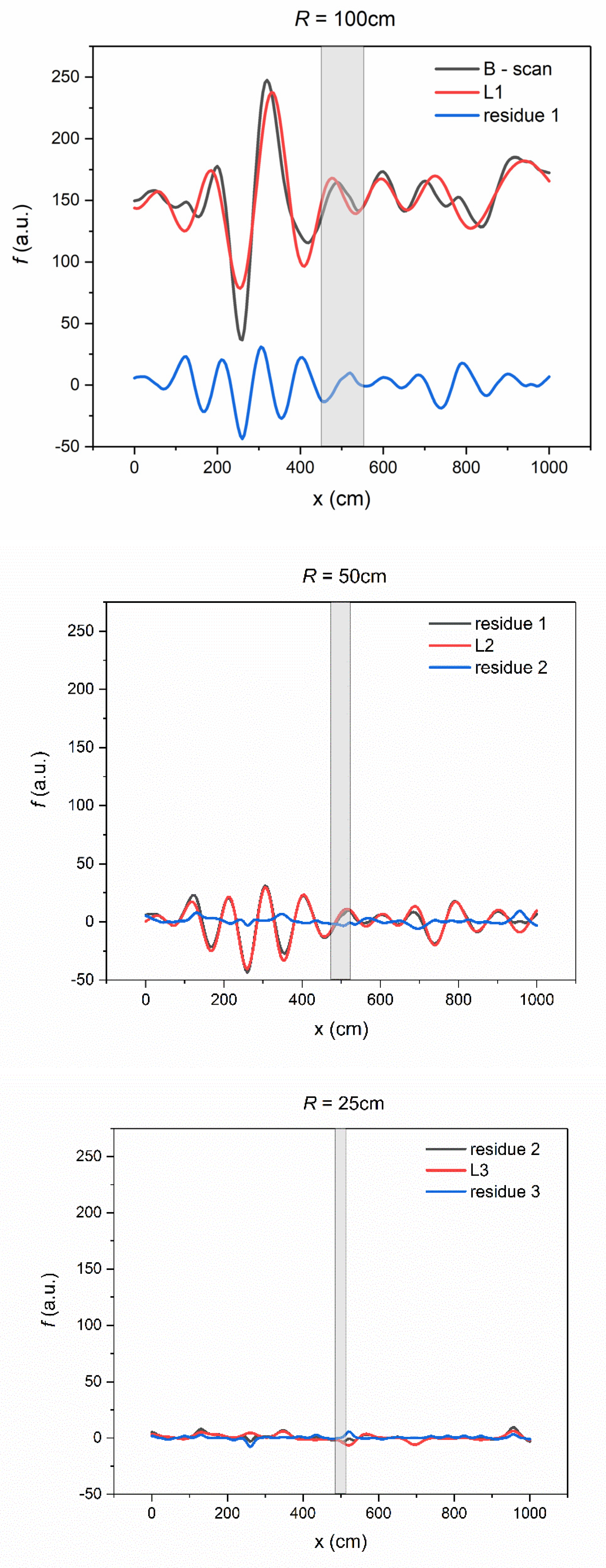
Figure 2 shows an example of B-scan and a method of approximation by a hierarchical model. Subsequent layers have a radius that is twice as small and explain the residues after the previous layer. As the radius decreases, the finer details of the B-scan are reproduced.

The hierarchical algorithm has several significant advantages:

• Gaussian CS-RBFs produce linear systems with sparse matrices, enabling the use of the sparse LSQR solver, which can work with the rank defect matrix;
• The time of the model building depends on the number of points, N, as N logN in contrast to simple RBF’s implementations with O(N³) efficiency;
• An iterative algorithm (successive layers correct the errors of the previous ones) creates a robust model, even with a very large initial radius. Successive layers have smaller radii and correct the inaccuracy introduced by the previous layer;
• The multi-layer model allows for control smoothing both by changing the regularisation coefficient and by a different number of layers.

6. Experimental Results

An example worth highlighting are the raw results of the archeological survey made in Płońsk, Poland, between Przejazd and 19 Stycznia streets at the old graveyard. The measurements were obtained using a 600 MHz impulse GPR system with bow-tie antennas. The investigated area was divided into subfragments, and the scans were realised on paths every 5 or 40 cm depending on terrain conditions. This gave about 200 scans for each subfragment. A drawing of one of the subfragments and an example of the one-path scanning result (B-scan) is shown in Figure 3.

Every measurement point contains 256 numbers describing GPR echoes from subsequent depths (A-scan). The set of subsequent A-scans makes the B-scan. To each of the A-scan numbers, the spatial coordinates x, y are added to obtain a 3D array. This makes cross-sections called C-scans. To illustrate the operation of the proposed method, one C-scan from a 1 m depth was made.

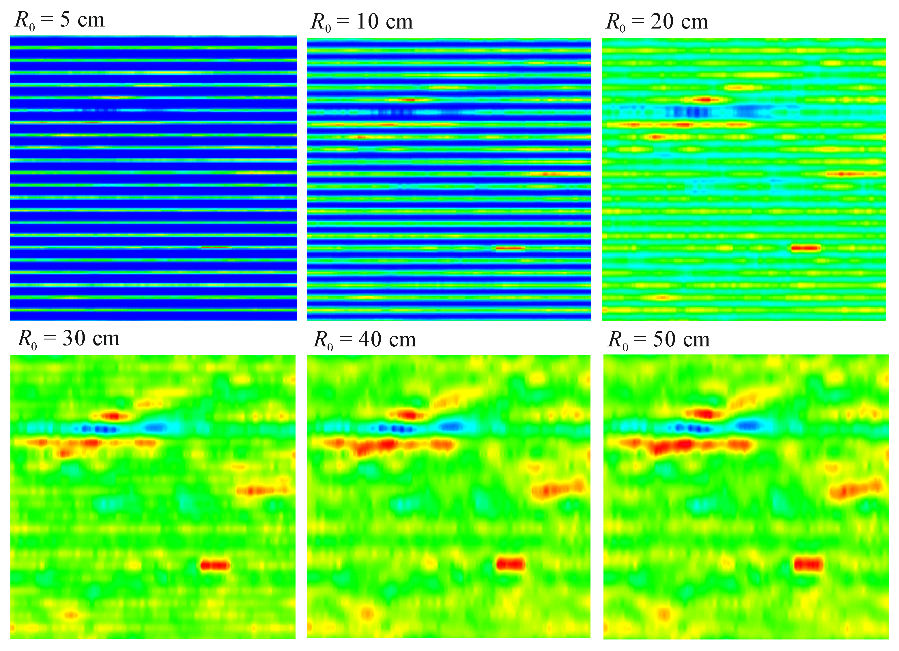
In order to use the hierarchical algorithm, three parameters must be chosen: the initial radius, R₀, the number of layers, N_L, in the model and the regularisation coefficient, λ. The main parameter affecting the quality of the approximation is the initial radius. Figure 4 shows the set of C-scans of 1 m depth for six different radius values. The other calculation parameters are N_L = 3, λ = 0, and the step of the mesh, which is equal to 5 cm.

In the two first C-scans (R₀ = 5 and 10 cm), the empty lines along the scanning paths can be observed. An approximation of the areas between the paths starts properly from a radius value of R₀ = 30 cm because it is the minimal radius value for which the empty areas can be approximated with points coming from two adjacent paths. A further increase in radius sharpens the image and enhances detail, but it does not change the shape of the objects. For R₀ ≥ 50 cm, these changes are almost imperceptible.

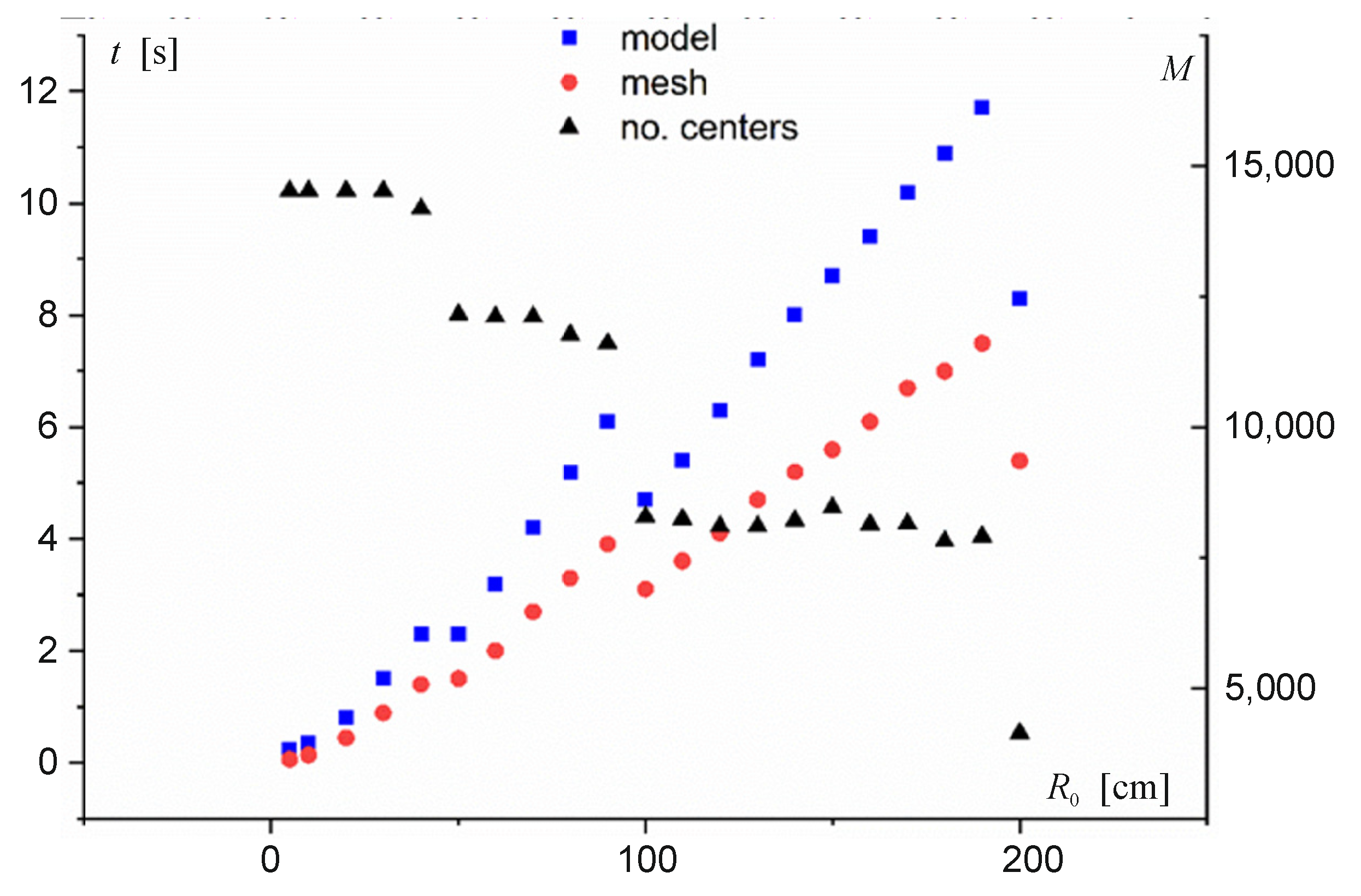
The value of the approximation radius decisively affects the calculation time. Figure 5 shows the calculation times of the model and function evaluation in the mesh nodes depending on R₀. Obviously, the computation time of the points on the mesh depends on its density and is proportional to the number of mesh nodes. All calculations were made for a rectangular mesh with equidistant nodes in the x and y directions, with a step of 5 cm. Calculations were performed on a computer with Intel Core i5-7200U CPU 2.5 GHz, 8 GB RAM on a Windows 10 operating system.

The computation time increases linearly in intervals with increasing radius. For radii at which there is an increase in computational speed, the number of points analysed decreases. This is because the hierarchical RBF model removes excessive (too dense) nodes from the model. The support radius parameter R_SUP is used to evaluate which points need to be removed and which do not. If two points are less than R_SUP·R_CURRENT units of distance apart, one of them is removed from the model. The larger the support radius, the faster the model construction and evaluation. However, values that are too large cause models to be “bumpy.” Recommended values for the support radius coefficient are in the range of 0.1–0.4, with 0.1 being the default value.

In the analysed case, where the distances between adjacent B-scans are 40 cm, the corresponding value of the initial radius is approximately 50 cm.

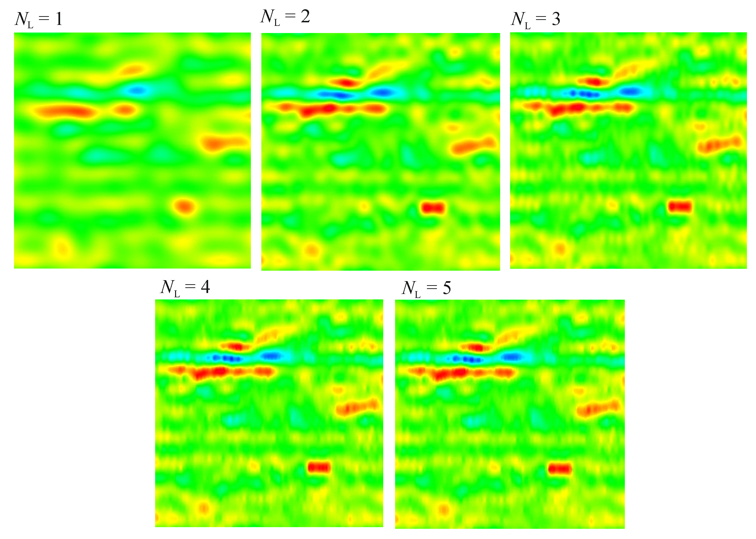
The second important parameter included in the model is the number of layers.

Table 2. The influence of the number of model layers on the approximation quality.

Layer Number	50 cm			100 cm			200 cm
	ERMS	EMAX	M	ERMS	EMAX	M	ERMS	EMAX	M
1	4.93	40.68	2474	15.82	81.39	1682	25.17	137.13	1001
2	3.38	33.64	7316	4.94	40.63	3440	15.89	82.96	2122
3	1.98	15.34	12,158	3.38	33.61	8282	4.49	40.59	4138
4	0.00	0.00	17,000	1.98	15.34	13124	3.38	33.65	8980
5	0.00	0.00	21,842	0.00	0.00	17966	1.98	15.36	13,822
6	0.00	0.00	26,684	0.00	0.00	2208	0.00	0.00	18,664

shows the effect of the number of layers on the approximation errors for the three R₀ values. Example C-scans for R₀ = 100 cm are shown in Figure 6.

With the increase in the number of layers, we observe a drop in approximation errors down to zero, but this is done at the expense of the computation complexity (increase in M). By choosing larger initial radii, more layers are needed to obtain an accurate surface representation.

The optimal number of layers can be estimated from the relation $N_L=\mathrm{round}\left[\ln \left(2R_0/\overline{r}\right)/\ln \left(2\right)\right]+2$, where $\overline{r}$ is the average distance between consecutive points in the B-scan. This selection ensures that the model is flexible enough to accurately reproduce the input data.

Another parameter that occurs in the hierarchical RBF model is the regularisation coefficient λ, which can take values of ≥0. This parameter adds controllable smoothing to the problem, which may reduce noise. Specification of a non-zero lambda means that in addition to fitting error solver also minimise $\lambda {\left[S^{″}\left(x\right)\right]}^2$, where S″(x) is the second derivative of squared error S. Specification of an exactly zero value means that no penalty is added. The optimal lambda is problem-dependent and requires trial and error. The recommended λ starting value is in the of range 10⁻⁵ to 10⁻⁶, which corresponds to a slightly noticeable smoothing of the function. A value of 0.01 usually means that strong smoothing is being used.

Calculation of nonlinearity penalty is costly: it results in a several-fold increase in the model construction time, but the evaluation time remains the same. In the example, the model building time increased by about 2.5-fold compared to the calculations for λ = 0 and did not depend on the value of λ > 0. However, since function smoothing can also be achieved by reducing the number of model layers, which reduces the computation time, the second solution is preferable.

7. Comparison of Gaussian CS-RBF with Other Approximation Methods

There are several methods of assessing the quality of the approximating function. The simplest is the root mean square error over N evaluation points x, as follows:

$$E_{\mathrm{RMS}}=\sqrt{\frac{1}{N}{{\displaystyle \sum _{j=1}^N\left[f\left({\mathit{x}}_j\right)-h\left({\mathit{x}}_j\right)\right]}}^2}$$

(11)

where $f\left(\mathit{x}\right)$ is the evaluated function and $h\left(\mathit{x}\right)$ is a measurement value.

The second is leave-one-out-cross-validation (LOOCV) [23]. In practical problems of scattered data interpolation, the exact solution is most likely unknown. In such situations, it is not possible to calculate the exact RMS error. Cross-validation is a statistical approach. One round of cross-validation involves partitioning a sample of data into complementary subsets, performing the analysis on one subset (training set), and validating the analysis on the other subset (validation set or testing set). To reduce variability, in most methods multiple rounds of cross-validation are performed using different partitions, and the validation results are combined (e.g., averaged) over the rounds to provide an estimate of the model’s predictive performance [24].

Another evaluation method is benchmark tests that sample and reconstruct test functions, such as Franke’s function [25].

GRP scans are a specific set of data for which we can determine an exact approximating function along the scan path, but large errors between paths are to be expected. LOOCV is not a good method for evaluating the quality of the approximating function since both training set and testing set will come from the scan path. Therefore, a custom test function that contains a point object and three longitudinal objects of different orientation and width was created (Figure 7). This function is described by the following formula:

$$f\left(x,y\right)={\displaystyle \sum _{i=1}^4{a}_i\exp \left[\frac{\left(b_{1i}x+c_{1i}\right)}{d_{1i}}+\frac{\left(b_{2i}y+c_{2i}\right)}{d_{2i}}\right]}$$

(12)

with the following coefficients:

i	a	b1	c1	d1	b2	c2	d2
1	0.75	60	−5	−4	60	−5	−4
2	0.75	100	−20	−10	9	−6	−10
3	0.5	9	−7	−4	30	−8	−4
4	0.2	9	−4	−11	9	−7	−1

For this test function, different RBF approximation methods available in Surfer [9] were compared. Model building was performed for a dataset typical of a B-scan GPR containing 4785 measurement points. Model evaluation was performed on the grid x = 0, …, 1, y = 0, …, 1, with a step of 0.02. Calculations were performed for different approximation radii. The E_RMS decreased with increasing radius to a value of around R₀² = 2 × 10⁻⁴, after which further increasing the radius slightly affected the quality of the test function representation. For such a radius, all E_RMS values were in the range of 2.1 × 10⁻³ to 2.5 × 10⁻³, while E_MAX was in the range of 0.036–0.044. The model building times for compactly supported Gaussian RBFs and other RBFs implemented in Surfer are shown in

Table 3. Model building times for different RBFs at R₀² = 0.002.

RBF	CS Gaussian	Multiqiadratic	Inverse Multiquadratic	Multilog	Natural Cubic Spline	TPS
t [s]	3.0	140.1	126.6	133.0	140.0	142.9

.

A similar analysis was performed for other models available in the Surfer package.

Table 4. Model building times and estimation errors of the test function for Gaussian CS-RBF and other models included in the Surfer program.

Model	Gaussian CS-RBF	Minimum Curvature	Triangulation with Linear Interpola-Tion	Kriging	IDP –Inverse Distance to a Power	Natural Neigh-Bor	Nearest Neigh-Bor	Local Polynomial
t × 103 [s]	3.0	0.14	0.02	2.9	0.18	1.1	0.02	0.27
ERMS	2.1	2.4	5.6	6.7	22	14	22	48
EMAX	44	33	99	98	266	307	355	534

shows the model building times and model estimation errors according to increasing E_RMS. The calculations were performed for the default parameters, set in the Surfer program, because their changes did not bring significant improvement in the quality of approximation.

Based on the results obtained, it can be concluded that the Gaussian CS-RBF approximation provides a representation quality of test function comparable to the minimum curvature (CS) method and significantly better than the other methods implemented in Surfer. However, the model building time is clearly longer than for most of these methods. In contrast, within the radial basis function approximation (Table 3), Gaussian CS-RBFs provide almost 50 times faster computation speed than for global RBFs.

8. Conclusions

This paper investigates the feasibility of using RBF approximation to create C-scans in GPR measurements. For this purpose, hierarchical approximation with compactly supported Gaussian RBF was used. The method is a part of the linear algebra library ALGLIB [12]. The algorithm is optimised in terms of computation time and memory usage, which gives the ability to handle millions of points on an ordinary PC.

Calculations were carried out for real data, including c.a. 5000 measurement points, and the optimal input parameters were selected. It was found that for these parameters the time needed to generate an image of one C-scan layer was about 5 s on a common computer. This is a relatively long time; however, it analyses data that often comes from several hours of field measurements. In addition, this time can be significantly reduced by settling for an image of slightly lower quality.

The use of Gaussian CS-RBFs enables multiple reductions in computation time compared to global RBFs with the same quality of surface representation. Compared to other commonly used methods, Gaussian CS-RBFs provide a very good approximation of the specific datasets that are obtained from GPR measurements. This is carried out at the cost of slightly higher computation time.

The presented hierarchical RBF approximation algorithm is one of the most efficient algorithms for processing large, scattered data sets. Its implementation, located in the ALGLIB library, enables simple software development, which can be successfully used to analyse GPR images.