Pre-Processing Filter Reflecting Human Visual Perception to Improve Saliency Detection Performance

Abstract

Salient object detection is a method of finding an object within an image that a person determines to be important and is expected to focus on. Various features are used to compute the visual saliency, and in general, the color and luminance of the scene are widely used among the spatial features. However, humans perceive the same color and luminance differently depending on the influence of the surrounding environment. As the human visual system (HVS) operates through a very complex mechanism, both neurobiological and psychological aspects must be considered for the accurate detection of salient objects. To reflect this characteristic in the saliency detection process, we have proposed two pre-processing methods to apply to the input image. First, we applied a bilateral filter to improve the segmentation results by smoothing the image so that only the overall context of the image remains while preserving the important borders of the image. Second, although the amount of light is the same, it can be perceived with a difference in the brightness owing to the influence of the surrounding environment. Therefore, we applied oriented difference-of-Gaussians (ODOG) and locally normalized ODOG (LODOG) filters that adjust the input image by predicting the brightness as perceived by humans. Experiments on five public benchmark datasets for which ground truth exists show that our proposed method further improves the performance of previous state-of-the-art methods.

1. Introduction

The information received from the human visual system (HVS) constitutes a significant proportion of all information received during the daytime [1]. Although the human brain can process large amounts of information, human visual information exceeds this processing capacity. Therefore, HVS discriminately processes large amounts of visual information by classifying them according to their importance [2,3,4,5]. Through this process, humans concentrate on areas with high importance, which are called salient regions. The saliency detection method refers to a computational model that quantifies a salient area or detects objects in an image by emulating a human’s selective visual attention mechanism.

Various methods were proposed to predict the areas where human attention is concentrated while staring at images or video scenes. Itti et al. [6] proposed a saliency detection algorithm that combines color, intensity, and orientation features in a center-surround manner based on feature integration theory. Harel et al. [7] proposed a graph-based method that combines the activation maps formed using feature vectors. Hou et al. [8] proposed a method for generating a saliency map using the spectral residuals obtained by considering the statistical characteristics of a natural image in the spectral domain.

Object-based saliency detection methods were also proposed from a different perspective from location-based methods. Liu et al. [9] segmented images to obtain regions of interest (ROIs) using density-based clustering and calculated the region saliency map based on the color, region size and location in the image. Cheng et al. [10] calculated the saliency value of the region using the measured global contrast score, but considering the influence of the contrast and spatial distance to the surrounding region that gains human attention. Li et al. [11] adopted a superpixel segmentation method and treated the saliency values of all regions as the optimization objective for each image rather than mapping visual features to saliency values with a unified model.

In order to perform quantitative comparisons on the performance of saliency detection methods, different public datasets have been created according to location-based and object-based detection methods. For the location-based detection method, Einhäuser et al. [12], Bruce et al. [13], Judd et al. [14], and Achanta et al. [15] constitute the dataset. The ground truth image for each image is a record of randomly selected subjects wearing an eye tracking device and staring at the image on the display for a set period of time. For the object-based detection method, datasets named DUT-OMRON [16], ECSSD [17], MSRA10K [10,18,19,20], PASCAL-S [21,22,23], and THUR15K [24] have been mainly used. The ground truth image for this type of dataset is a pixel-level binary mask judged as a salient object by randomly selected experimenters watching the image.

For saliency detection, various features that can be obtained from the scene are used. Among them, color and luminance, which are spatial characteristics of a scene, are mainly used because they are intuitive and easy to obtain. However, humans do not perceive visual stimuli as absolute values, but as relative values affected by surrounding information, causing an visual illusion [25,26,27,28,29]. This means that the result of detecting saliency by using the original image data without any processing may not effectively reflect the visual illusion of such a human. Therefore, it is necessary to process the features obtained from the image in consideration of the human’s neurobiological and psychological mechanisms of visual perception.

In this study, we verified the effect of applying a pre-filter that reflects the human visual perception system to the dataset used in the saliency detection method. We approached it from the following two perspectives:

• According to the visual perception model, the rapid initial analysis of visual features in the natural scene recognition process starts at low spatial frequencies following a “coarse-to-fine” sequence [30,31,32,33]. In other words, when recognizing a scene, it first accepts the overall characteristics of the whole scene, and then recognizes the detailed characteristics. Saliency detection is a technology that detects an area or object that a person will pay attention to when facing a scene. Therefore, it is necessary to pay attention to the overall features rather than the details of the scene in consideration of the human scene recognition process. In addition, the performance of the superpixel method used as a segmentation method in saliency detection is judged by the similarity of pixels constituting each superpixel and whether the edge in the actual image is reflected. In order to satisfy both requirements, it is necessary to remove minute differences in pixel values while maintaining important edges. Therefore, if an edge-preserving filter is applied to the original image before performing superpixel segmentation, the segmentation result and saliency detection performance can be expected to improve.
• Simultaneous contrast effect is a visual illusion that perceives the same gray color differently depending on the brightness of the background. Studies that approach this visual illusion as a low-level process have analyzed that simple interactions between adjacent neurons are caused by simple filters implementing lateral inhibition in the early stages of the visual system, where they are performed [34,35,36,37,38]. In addition, various methods have been proposed to predict the brightness perceived by humans under the influence of visual illusions [39,40,41,42,43]. The ground truth image used to compare the performance of the saliency detection method is the result of the perception of brightness as the subject observes the image and creates it manually. Nevertheless, because the input image uses the original pixel-specific data as it is, it is used without considering human visual characteristics. Therefore, a pre-processing method that considers the brightness perception of the input image is required.

The remainder of this paper is organized as follows: In Section 2, we introduce our method to verify the effects of the pre-filtered datasets. Section 3 presents our experimental results and analysis, and Section 4 concludes the paper.

2. Proposed Methodology

This section describes two pre-processing filters that can be applied to improve saliency detection performance:

• Bilateral filter: Both the foreground and the background in the image do not exist as a single pixel, and have meaning by clusters of pixels of similar color and brightness in a certain area. The superpixel-based saliency detection method focuses on this characteristic and divides the image into superpixels, which are clusters of similar pixels, and detects salient objects by considering the correlation of each cluster. The bilateral filter removes the detail within the clusters that degrades the correlation between superpixels. It also preserves prominent edges within the image so that the boundaries between superpixels better reflect real edges.
• Perceptual brightness prediction filter: In general, saliency detection methods use original data values of input images. However, since humans perceive relative brightness, stimulus distortion occurs in the scene recognition process. Since saliency detection is a technique for detecting areas or objects that humans judge to be salient, such stimulus distortion must be reflected in the detection process. The perceived brightness prediction filter calculates a relative brightness value that is actually perceived with respect to the light intensity obtained by the human eye.

More details on each filter are described in the following subsections.

2.1. Bilateral Filtering for Superpixel

In a natural image, although pixels that are spatially close to each other may appear to be identical, there exist slight differences in their values, which contribute to the rich details of the image. However, humans instantaneously acquire data from the scene and process it appropriately. In such a short time, the HVS ignores fine details and unnecessary edges in the scene and acquires the overall information that is necessary to understand the context of the scene. Therefore, it is more useful to process the image in units of superpixels, which represent perceptually meaningful pixels, than in units of pixels individually. Hence, several object-based saliency detection methods [11,16,44,45,46,47,48,49,50,51,52] mainly use the simple linear iterative clustering (SLIC) technique [53,54] to segment an image into superpixels. This technique uses a few parameters that can be easily adjusted and demonstrates reasonable segmentation results with a low computational cost.

However, although SLIC splits the image better than other state-of-the-art methods, it sometimes exhibits a jagged boundary on the actual image edges, as depicted in the upper row of Figure 1. To alleviate this problem and improve the superpixel result by removing the details in the image, we applied a bilateral filter [55,56,57,58], which is an edge-preserving filter.

The bilateral filter developed by Tomasi and Manduchi [55] is a nonlinear filter, in which the output is a weighted average of the input. This weight is based on a Gaussian distribution and depends on both the distance and intensity difference of the pixels. For input image I, the bilateral-filtered image $\widehat{I}$ at pixel $\mathbf{p}$ is obtained as

$$\begin{array}{c}\hfill {\widehat{I}}_{\mathbf{p}}=\frac{1}{W_{\mathbf{p}}}\sum _{\mathbf{q}\in S}^{}{G}_{{\sigma }_s}\left(∥\mathbf{p}-\mathbf{q}∥\right)G_{{\sigma }_r}\left(\left|I_{\mathbf{p}}-I_{\mathbf{q}}\right|\right)I_{\mathbf{q}}\\ \hfill \mathrm{w}\mathrm{h}\mathrm{e}\mathrm{r}\mathrm{e},W_{\mathbf{p}}=\sum _{\mathbf{q}\in S}^{}{G}_{{\sigma }_s}\left(∥\mathbf{p}-\mathbf{q}∥\right)G_{{\sigma }_r}\left(\left|I_{\mathbf{p}}-I_{\mathbf{q}}\right|\right)\end{array}$$

(1)

where $\mathbf{q}$ is the pixel inside the window mask S centered on $\mathbf{p}$, $G\left(·\right)$ is the Gaussian function, ${\sigma }_s$ and ${\sigma }_r$ are the standard deviations of space s and range r, specifying the amount of filtering on the image, and $∥·∥$ represent the Euclidean distance function. As can be seen from the comparison depicted in Figure 1a, the bilateral filter removes the delicate details while preserving the major edges of the image. Figure 1b,c depict the result of the bilateral filter smoothing of the boundaries of the superpixels, which significantly reflects the edges of the image.

2.2. Brightness Perception

Brightness refers to the apparent luminance of a patch in the image itself, whereas lightness refers to the apparent reflectance of a surface in a scene [25]. As humans respond to the proportion of the light reflected by an object rather than the total light reflected by an object, they perceive the relative reflectance of objects despite changes in the illumination, which is called the lightness constancy [28]. This means that humans do not absolutely perceive the brightness of the scene but rather perceive it relatively under the influence of the surrounding environment. A representative example of brightness perception is the checker shadow illusion [26], as depicted in Figure 2. Comparing the two blocks labeled A and B in Figure 2a, blocks A and B appear to consist of gray patches of different brightness. Although block B looks brighter than block A, as can be seen in Figure 2b, the luminance value of the two blocks in 8-bit grayscale is the same as 120.

To measure the degree of human perception of brightness within an image, we applied the oriented difference-of-Gaussians (ODOG) model [39,40,41,42,43]. The ODOG filter was designed by reflecting the principle of orientation selectivity [59] of a primary visual cortex (V1) simple cell, which is located in the first stage of the cortical processing of visual information. An anisotropic Gaussian filter was used to accumulate the strength in a desired orientation over the lateral geniculate nucleus (LGN) center-surround group with a response pattern in the form of a difference-of-Gaussians (DoG) [60]. The ODOG filter is defined as follows:

$$\begin{array}{c}\hfill f_{ODOG}\left({\sigma }_1,{\sigma }_2,\theta ;x,y\right)=\frac{1}{2\pi {\sigma }_1^2}exp\left(-\frac{u^2+v^2}{2{\sigma }_1^2}\right)-\frac{1}{2\pi {\sigma }_1{\sigma }_2}exp\left(-\frac{1}{2}\left(\frac{u^2}{{\sigma }_2^2}+\frac{v^2}{{\sigma }_1^2}\right)\right)\\ \hfill =\frac{1}{2\pi {\sigma }_1}exp\left(-\frac{v^2}{2{\sigma }_1^2}\right)\left(\frac{1}{{\sigma }_1}exp\left(-\frac{u^2}{2{\sigma }_1^2}\right)-\frac{1}{{\sigma }_2}exp\left(-\frac{u^2}{2{\sigma }_2^2}\right)\right)\end{array}$$

(2)

where ${\sigma }_1$, ${\sigma }_2$ are the standard deviations of the center and surrounding Gaussian functions, respectively. The parameter ${\sigma }_1$ is set to seven values arranged in octave intervals between 1.06 and 67.88 to reflect the space constants, and ${\sigma }_2$ is set as ${\sigma }_2=2{\sigma }_1$. The orientation of the filter $\theta$ has six components at ${30}^{\circ }$ intervals (from $0^{\circ }$ to ${150}^{\circ }$). The coordinates u, v rotated in the $\theta$ orientation for the x, y variables are given as follows:

$$\left[\begin{array}{c}u\\ v\end{array}\right]=\left[\begin{array}{cc}cos\left(\theta \right)& sin\left(\theta \right)\\ -sin\left(\theta \right)& cos\left(\theta \right)\end{array}\right]\left[\begin{array}{c}x\\ y\end{array}\right]$$

(3)

The input image was processed linearly using 42 filters generated by Equation (2). Thereafter, the weighted summations for each orientation $\theta$ were calculated, and the final result was obtained by averaging the normalized output values over all orientations.

The ODOG model applies the same weights to the energies in each orientation and sums them globally. Meanwhile, reference [41] reported that the global normalization in the ODOG model may not effectively reflect the brightness of the image; to compensate for this limitation, a locally normalized ODOG (LODOG) was proposed. The LODOG calculates the normalized root mean square (RMS) for a Gaussian weight window centered on each pixel.

A comparison of the images filtered by ODOG and LODOG is depicted in Figure 3. Figure 3b,c depict the predicted brightness values after applying each filter to the original image in Figure 3a in the RGB color space. The filtered images exhibit a slight color difference compared to the original image, and the contrast tends to increase. However, visual confirmation of the filtered image triggers a new perception of brightness. Therefore, in Figure 3d, the pixel level values at the horizontal position indicated by the red line at the center of the Figure 3a–c are compared. The x-axis of the graph represents the spatial location corresponding to the red line shown in Figure 3a–c, and the y-axis represents the pixel range. The blue solid line and the red dotted line are pixel values filtered through ODOG and LODOG, respectively. In the image, since the sneakers are centered on a dark background, the white sneakers stand out brighter and the dark background is perceived as relatively dark. In the case of the background, it is perceived as darker near the borderline adjacent to the bright sneakers, and is less affected the further away from the sneakers. The comparison with the original pixel values in the solid black line shows that the ODOG and LODOG filters predict the perceived brightness.

3. Experimental Results and Analysis

3.1. Datasets

The proposed method was applied to five public object-based datasets for comparison of saliency detection performance. The characteristics of each dataset are as follows:

DUT-OMRON dataset contains 5168 high-quality images that are manually selected from more than 140,000 images with one or more salient objects and a relatively complex background [16]. All of them were resized with a resolution of $400\times x$ or $x\times 400$, where x is less than 400. ECSSD dataset consists of 1000 images obtained from the internet, which typically contain natural images [17]. The selected images include semantically meaningful but structurally complex backgrounds. MSRA10K dataset generated by Cheng et al. [10] consisted of 10,000 images randomly selected from the MSRA dataset of more than 20,000 images provided by Liu et al. [61]. PASCAL-S dataset is built on the validation set of the PASCAL VOC 2010 segmentation challenge [21]. It contains 850 natural images with multiple objects in the scene [22,23]. THUR15K dataset consists of approximately 15,000 images classified by five keywords (butterfly, coffee mug, dog jump, giraffe, and plane) [24]. In each image, there is an unambiguous object that matches the query keyword and contains the correct content for most of the object to be displayed. As there is no ground truth for all images, only 6233 images for which ground truth images exist were used in the experiment.

Each dataset comes with ground truth images for salient objects. These ground truth images are binary masks, manually labeled by 3 to 12 subjects selected by the creators of each dataset.

3.2. Evaluation Metrics

For objective performance evaluation, we adopted precision–recall (PR) curve, area under the curve (AUC) score, and F-measure.

The PR curve is a plot with precision on the y-axis and recall on the x-axis for different probability thresholds. Precision(also known as positive predicted value) is the ratio of the correctly predicted salient regions out of all predicted salient regions. Recall (also known as the true positive rate or sensitivity) is the ratio of the correctly predicted salient region to the actual salient region. The precision and recall are calculated using the following equation:

$$precision=\frac{TP}{TP+FP}$$

(4)

$$recall=\frac{TP}{TP+FN}$$

(5)

where $TP$, $FP$, and $FN$ are the true positive, false positive, and false negative rates, respectively.

The AUC score measures the overall performance based on the area under the receiver operating characteristic (ROC) curve. The ROC curve is a plot with recall on the y-axis and a false positive rate (FPR) on the x-axis for different probability thresholds. FPR is calculated using the following equation:

$$FPR=\frac{FP}{FP+TN}$$

(6)

where $TN$ represents the true negative rates. The higher the performance of the saliency detection model, the closer the AUC score is to one, and the lower the performance of the saliency detection model, the closer the AUC score is to zero (i.e., the minimum AUC score is 0.5).

The F-measure is the weighted harmonic mean of precision and recall. It is also adopted to measure the overall performance of the saliency detection model and is calculated as follows:

$$F_{\beta }=\frac{(1+{\beta }^2)precision\times recall}{{\beta }^2\times precision+recall}$$

(7)

where the weighting parameter ${\beta }^2$ is set to one for our implementation.

3.3. Implementation Details

To verify the effectiveness of pre-processing filters performed on the input image on the saliency detection performance, we applied six saliency detection methods. All of these methods are superpixel-based salient object detection methods and are widely known and highly cited or recently published methods. The names of the six methods and the number of superpixels and compactness parameters for SLIC performed in each method were set as listed in

Table 1. Six methods used in the experiment and parameters for SLIC.

Method	Number of Superpixels	Compactness
MC [45]	250	20
GMR [16]	200	20
DSR [46]	[50, 100, 150, 200, 250, 300, 350, 400]	[10, 10, 20, 20, 25, 25, 30, 30]
HDCT [48]	500 pixels/superpixel	20
RBD [49]	600 pixels/superpixel	20
GLGOV [50]	200 pixels/superpixel	20

. The size of the mask S and the standard deviations ${\sigma }_s$ and ${\sigma }_r$ used for the bilateral filter in Equation (1) were $11\times 11$, 50 and 0.1, respectively. The bilateral filter was applied twice iteratively to the image.

3.4. Verification Framework

To verify that the filters described in Section 2.1 and Section 2.2 improve the saliency detection performance, we applied the filters both individually and in combination on the images.

Table 2. Names and descriptions of filters used for verification.

Name	Description
BF	Applying bilateral filter only
ODOG	Predicting perceived brightness using ODOG only
LODOG	Predicting perceived brightness using LODOG only
BF+ODOG	Applying a bilateral filter, and thereafter predicting by using ODOG
BF+LODOG	Applying a bilateral filter, and thereafter predicting by using LODOG

lists the names and descriptions of the filters applied to the images. The bilateral filter was applied iteratively to achieve a sufficient smoothing result as long as the edges were preserved. We also assumed that brightness interference occurs on a per-area basis rather than on a per-pixel basis. This means that the details of the scene are not important. Therefore, while combining two filters, the bilateral filter preceded the brightness perception filter.

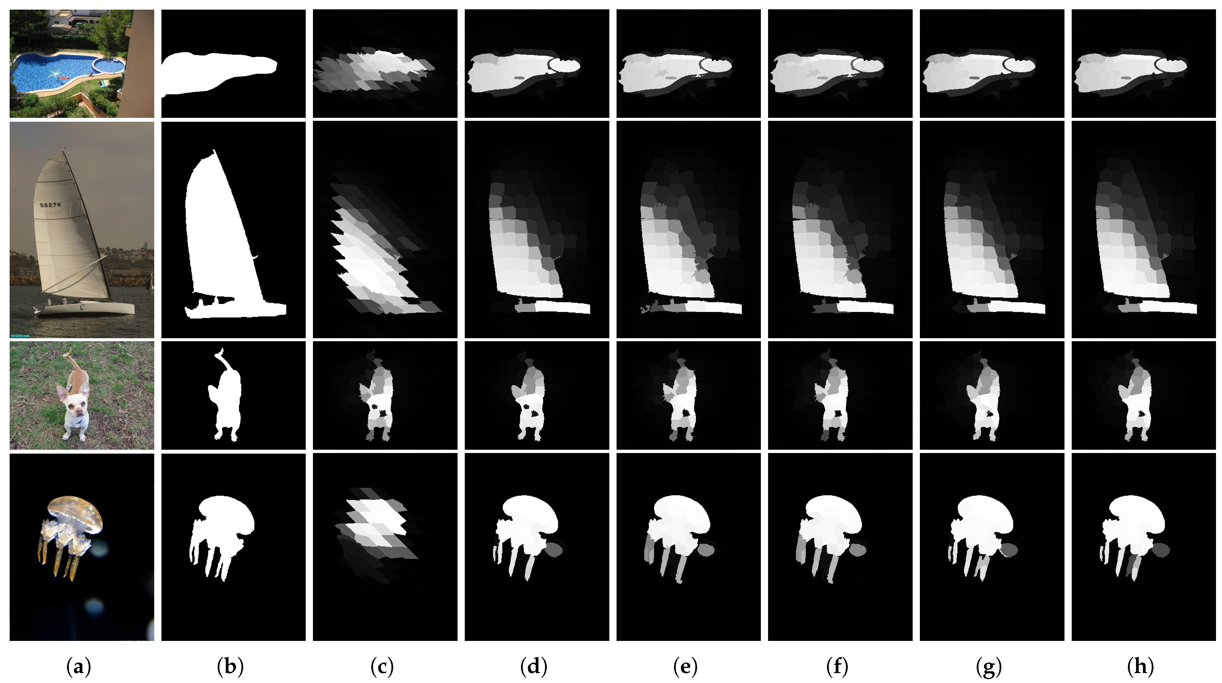
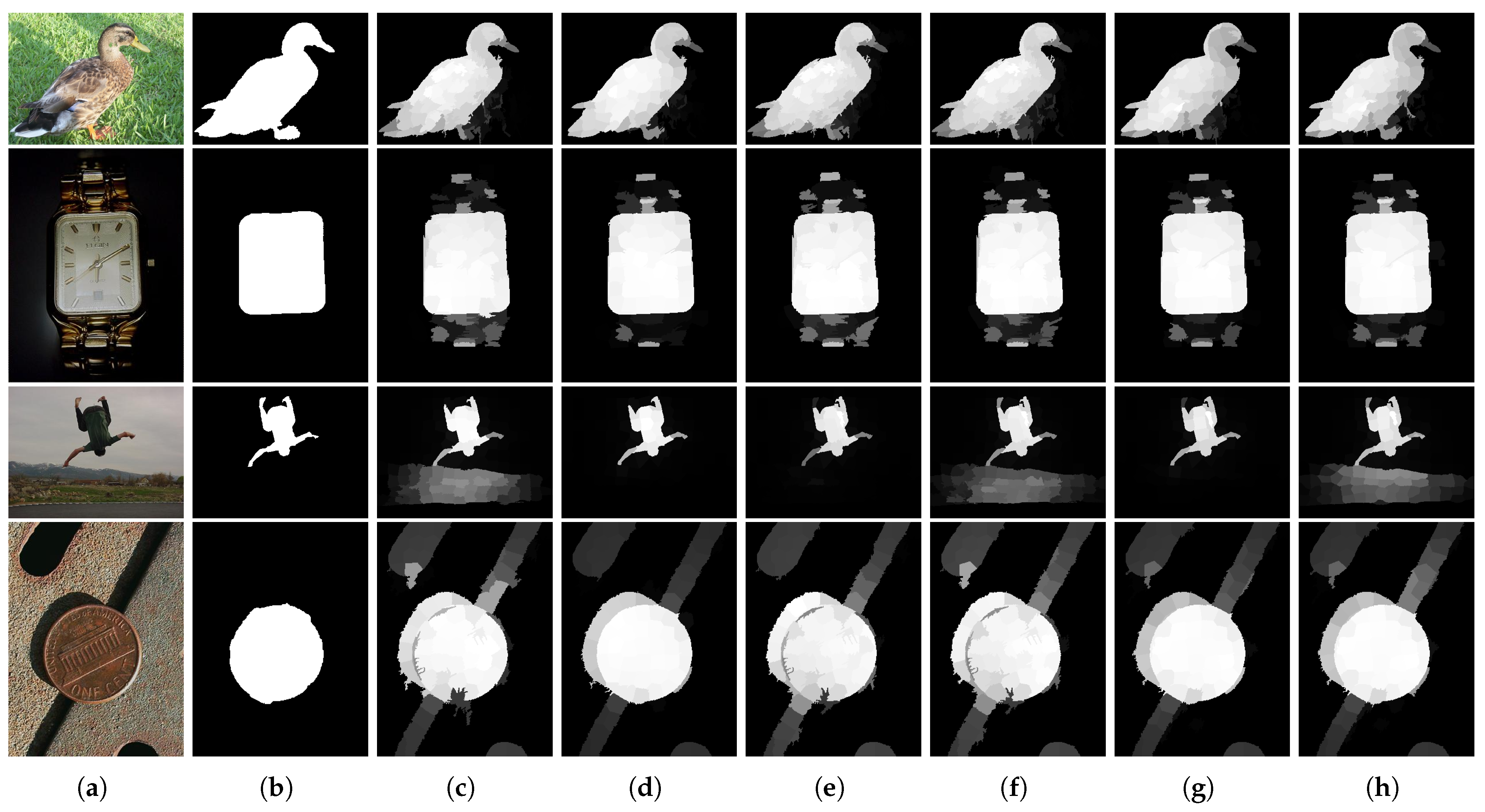
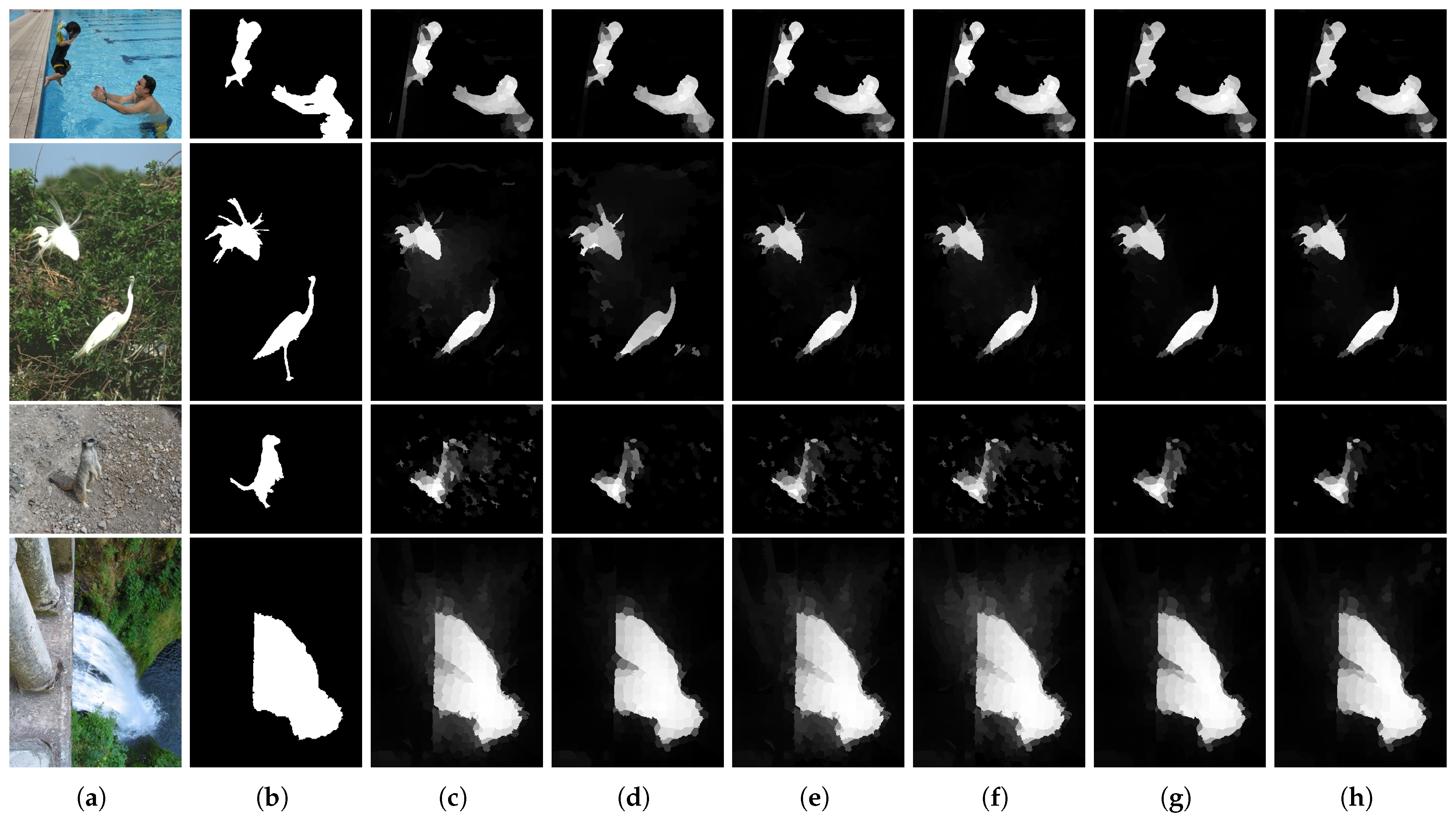
3.5. Subjective Quality Comparison

To evaluate the effectiveness of the proposed method, we demonstrated both subjective quality comparison and objective performance for all results with each algorithm applied to five datasets.

A subjective quality comparison is the process of comparing how similar the saliency map result generated by applying the saliency detection method to the input image is with the ground truth image. In this process, different saliency detection methods can be compared by paying attention to the shape of the salient object, the shape of superpixels, and the brightness, which means the degree of saliency. To effectively compare the results of the proposed method applied to each saliency detection method, several examples are depicted in Figure 4, Figure 5, Figure 6, Figure 7, Figure 8 and Figure 9. Columns (a) and (b) depict the input image and the ground truth image, respectively. Column (c) depicts the saliency detection results obtained through the existing algorithm without any pre-processing. First, as depicted in column (d), the jagged patterns existing at the boundary line between the superpixels are significantly reduced by the bilateral filter, as intended. This reflects the boundary line between the object and the background more effectively, which can be seen in the original image and the ground truth image. Second, the effects of ODOG and LODOG are depicted in columns (e) and (f), respectively. Both filters produce an image with a brightness value affected by the surrounding area. This is similar to the effect of increasing the contrast ratio of an image. Therefore, it can be seen that the greater the difference in contrast between the salient object and the background, the greater the influence of the filters. Third, the effects of ODOG and LODOG combined with bilateral filters are depicted in columns (g) and (h), respectively. Although there are differences depending on the characteristics of the input image, it is possible to confirm that the advantages that can be obtained through each filter are effectively combined.

The results indicate that the proposed method is effective for all saliency detection methods. In particular, when applied to GMR and DSR, it exhibited the most noticeable improvement in results. In the first, second, and fourth rows of Figure 5 and the first and second rows of Figure 6, the results produced by the two methods are significantly different from the shape of the salient object. However, after applying the proposed method, the overall silhouette of the salient object present in the image appears.

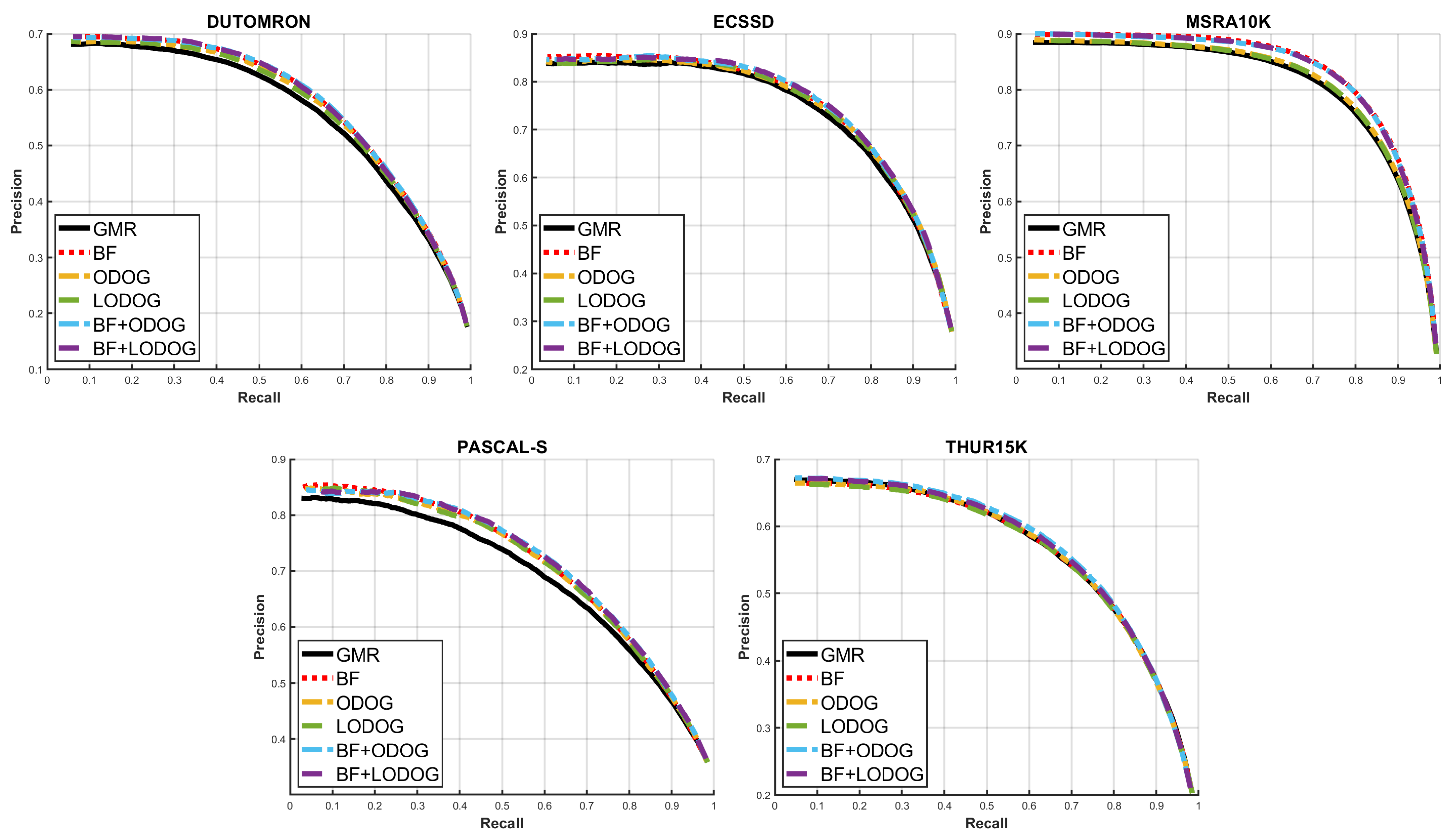
3.6. Objective Performance Comparison

To objectively compare the performance of the proposed method, we first demonstrated the PR curves as depicted in Figure 10, Figure 11, Figure 12, Figure 13, Figure 14 and Figure 15. First, in the case of the MC and RBD mehods depicted in Figure 10 and Figure 14, the results of the five pre-processing methods are similar to or slightly improved in all datasets. In particular, through PASCAL-S, the MC method demonstrated that ODOG produces better results than other pre-processing methods, and the RBD method demonstrated that it is advantageous to combine BF and brightness perception filters. Furthermore, Figure 11 and Figure 12 show that the proposed method exhibits a noticeable performance improvement when applied to the GMR and DSR methods. In the case of the GMR method, except for THUR15K, all pre-processing methods led to effective performance improvements, and in the DSR method, BF exhibited an effective improvement compared to other pre-processing methods in all datasets. In Figure 13, it is shown that only ODOG and LODOG have similar performances to the existing HDCT method in the datasets excluding THUR15K. Finally, in Figure 15, GLGOV exhibited improved effects on ECSSD, PASCAL-S, and THUR15K when BF and brightness perception filters were applied together, similar to RBD.

To numerically evaluate the performance of our approach, we additionally compared the AUC and F-measure using the method proposed in [15]. The results of the two measurements are listed in

Table 3. AUC score comparison for each method used in the experiment. Red and blue indicate the best and second performances, respectively.

Method	Dataset	Original	BF	ODOG	LODOG	BF+ODOG	BF+LODOG
MC [45]	DUT-OMRON	0.8876	0.8864	0.8886	0.8879	0.8876	0.8875
	ECSSD	0.9247	0.9243	0.9252	0.9251	0.9269	0.9264
	MSRA10K	0.9552	0.9550	0.9550	0.9547	0.9551	0.9543
	PASCAL-S	0.8639	0.8622	0.8627	0.8641	0.8633	0.8630
	THUR15K	0.9138	0.9131	0.9137	0.9138	0.9136	0.9133
	Avg.	0.9090	0.9082	0.9091	0.9091	0.9093	0.9089
GMR [16]	DUT-OMRON	0.8452	0.8506	0.8496	0.8480	0.8504	0.8507
	ECSSD	0.9101	0.9139	0.9140	0.9143	0.9163	0.9168
	MSRA10K	0.9167	0.9268	0.9190	0.9185	0.9257	0.9260
	PASCAL-S	0.8237	0.8347	0.8329	0.8348	0.8370	0.8373
	THUR15K	0.8843	0.8835	0.8838	0.8836	0.8853	0.8854
	Avg.	0.8760	0.8819	0.8799	0.8799	0.8829	0.8832
DSR [46]	DUT-OMRON	0.8907	0.8919	0.8932	0.8926	0.8904	0.8897
	ECSSD	0.9120	0.9160	0.9118	0.9119	0.9128	0.9132
	MSRA10K	0.9526	0.9536	0.9533	0.9526	0.9515	0.9515
	PASCAL-S	0.8495	0.8527	0.8526	0.8527	0.8525	0.8520
	THUR15K	0.9006	0.9006	0.9009	0.8996	0.8991	0.8978
	Avg.	0.9011	0.9030	0.9024	0.9019	0.9013	0.9009
HDCT [48]	DUT-OMRON	0.8996	0.8856	0.9005	0.9000	0.8900	0.8898
	ECSSD	0.9150	0.8968	0.9167	0.9163	0.9028	0.9028
	MSRA10K	0.9641	0.9538	0.9640	0.9638	0.9567	0.9567
	PASCAL-S	0.8538	0.8404	0.8582	0.8582	0.8482	0.8475
	THUR15K	0.9049	0.8993	0.9052	0.9045	0.9014	0.9007
	Avg.	0.9075	0.8952	0.9089	0.9085	0.8998	0.8995
RBD [49]	DUT-OMRON	0.8920	0.8921	0.8922	0.8921	0.8922	0.8924
	ECSSD	0.9010	0.8992	0.8995	0.8999	0.8998	0.9011
	MSRA10K	0.9548	0.9545	0.9541	0.9542	0.9549	0.9549
	PASCAL-S	0.8526	0.8517	0.8543	0.8549	0.8535	0.8554
	THUR15K	0.8901	0.8895	0.8915	0.8914	0.8918	0.8920
	Avg.	0.8981	0.8974	0.8983	0.8985	0.8985	0.8992
GLGOV [50]	DUT-OMRON	0.8932	0.8928	0.8934	0.8933	0.8934	0.8929
	ECSSD	0.9145	0.9176	0.9150	0.9149	0.9181	0.9188
	MSRA10K	0.9665	0.9656	0.9659	0.9658	0.9658	0.9659
	PASCAL-S	0.8625	0.8643	0.8639	0.8641	0.8655	0.8661
	THUR15K	0.9063	0.9064	0.9064	0.9063	0.9073	0.9070
	Avg.	0.9086	0.9094	0.9089	0.9089	0.9100	0.9101

and

Table 4. F-measure comparison for each method used in the experiment. Red and blue indicate the best and second performances, respectively.

Method	Dataset	Original	BF	ODOG	LODOG	BF+ODOG	BF+LODOG
MC [45]	DUT-OMRON	0.5360	0.5381	0.5384	0.5382	0.5410	0.5413
	ECSSD	0.6583	0.6583	0.6593	0.6595	0.6615	0.6617
	MSRA10K	0.7944	0.7938	0.7947	0.7952	0.7959	0.7953
	PASCAL-S	0.5540	0.5516	0.5567	0.5598	0.5538	0.5563
	THUR15K	0.5572	0.5583	0.5582	0.5578	0.5607	0.5598
	Avg.	0.6200	0.6201	0.6215	0.6221	0.6226	0.6229
GMR [16]	DUT-OMRON	0.5042	0.5193	0.5145	0.5114	0.5204	0.5183
	ECSSD	0.6389	0.6508	0.6494	0.6482	0.6514	0.6553
	MSRA10K	0.7082	0.7334	0.7136	0.7137	0.7309	0.7322
	PASCAL-S	0.5137	0.5305	0.5299	0.5306	0.5337	0.5353
	THUR15K	0.5312	0.5315	0.5296	0.5285	0.5355	0.5348
	Avg.	0.5792	0.5931	0.5874	0.5865	0.5944	0.5952
DSR [46]	DUT-OMRON	0.5257	0.5331	0.5314	0.5299	0.5310	0.5299
	ECSSD	0.6460	0.6559	0.6462	0.6457	0.6469	0.6479
	MSRA10K	0.7646	0.7758	0.7674	0.7668	0.7673	0.7681
	PASCAL-S	0.5497	0.5568	0.5519	0.5524	0.5541	0.5538
	THUR15K	0.5465	0.5482	0.5458	0.5443	0.5475	0.5459
	Avg.	0.6065	0.6140	0.6085	0.6078	0.6094	0.6091
HDCT [48]	DUT-OMRON	0.5358	0.5172	0.5342	0.5340	0.5226	0.5223
	ECSSD	0.6487	0.6162	0.6508	0.6507	0.6269	0.6256
	MSRA10K	0.7916	0.7689	0.7908	0.7900	0.7768	0.7761
	PASCAL-S	0.5418	0.5178	0.5510	0.5499	0.5296	0.5290
	THUR15K	0.5567	0.5505	0.5560	0.5552	0.5522	0.5515
	Avg.	0.6149	0.5941	0.6166	0.6160	0.6016	0.6009
RBD [49]	DUT-OMRON	0.5411	0.5436	0.5425	0.5418	0.5448	0.5440
	ECSSD	0.6503	0.6529	0.6493	0.6499	0.6546	0.6544
	MSRA10K	0.8073	0.8078	0.8069	0.8066	0.8081	0.8083
	PASCAL-S	0.5768	0.5761	0.5819	0.5808	0.5803	0.5809
	THUR15K	0.5424	0.5441	0.5454	0.5440	0.5489	0.5476
	Avg.	0.6236	0.6249	0.6252	0.6246	0.6273	0.6270
GLGOV [50]	DUT-OMRON	0.5445	0.5470	0.5443	0.5432	0.5460	0.5460
	ECSSD	0.6917	0.6935	0.6919	0.6910	0.6971	0.6961
	MSRA10K	0.8381	0.8369	0.8386	0.8379	0.8379	0.8380
	PASCAL-S	0.6031	0.6021	0.6057	0.6065	0.6061	0.6066
	THUR15K	0.5732	0.5786	0.5743	0.5730	0.5795	0.5785
	Avg.	0.6501	0.6516	0.6510	0.6503	0.6533	0.6530

. It should be noted that the red and blue scores listed in the table represent the first and second performances, respectively. Although there are minor differences in the combination of detection methods and datasets, in general, the performance improves when the proposed pre-processing filter is applied. The most pronounced improvement is seen in the GMR and DSR methods, as in the subjective quality comparison. In the case of the GMR method, the differences between the best case and the original for AUC and F-measure were 0.0072 and 0.0160, and for the DSR method, these values were 0.0019 and 0.0075, respectively. Unlike other detection methods, the HDCT method exhibits the best effect when only the brightness perception filter is applied. The remaining detection methods are generally more effective when BF and brightness perception filters are combined.

4. Conclusions

In this paper, we proposed a method of applying a pre-processing filter that considers human visual perception characteristics to improve the protrusion detection performance. The pre-processing filters were used individually or in combination depending on the purpose. The experimental results with five publicly available data sets have shown that our method effectively improves the performance of six superpixel-based saliency detection methods. Further evaluation with a PR curve, AUC, and F-measure have also confirmed the effectiveness of the proposed approach. We have found several advantages in terms of saliency detection performance by applying the proposed method. First, the bilateral filter smooths the detail component while preserving the edges of the image. The flattened image increases the similarity both within and between each superpixel. The superpixel-based saliency detection method detects salient objects through superpixel correlation, which leads to an improved performance. Second, the salient object contains stimulus components that are distinct from the surrounding environment. An easily perceived difference is the brightness of the scene. Humans receive this component as a distorted value because it is interfered with by the ambient luminance when acquiring it. Therefore, the brightness component obtained through the cognitive brightness prediction filter amplifies the difference between the salient object and the background to a level perceived by humans. This leads to a decrease in the correlation between the salient object and the background. When humans detect salient objects, it is known that the bottom-up and top-down methods finally combine to put the visual recognition system into action. Recently, top-down methods for training deep neural networks using salient datasets and the detection of salient objects in images through this trained network is being actively studied. For future work, we will focus on bottom-up saliency detection methods that work in conjunction with pre-processing filters to improve performance and their combination with top-down methods.

References

1. Li, J.; Gao, W. Visual Saliency Computation: A Machine Learning Perspective; Springer: Cham, Switzerland, 2014. [Google Scholar]
2. Shepherd, G.M. The Synaptic Organization of the Brain; Oxford University Press: Oxford, UK, 2004. [Google Scholar]
3. Koch, C. Biophysics of Computation: Information Processing in Single Neurons; Oxford University Press: Oxford, UK, 2004. [Google Scholar]
4. Raichle, M.E. The brain’s dark energy. Sci. Am. 2010, 302, 44–49. [Google Scholar] [CrossRef]
5. Borji, A.; Itti, L. State-of-the-art in visual attention modeling. IEEE Trans. Pattern Anal. Mach. Intell. 2012, 35, 185–207. [Google Scholar] [CrossRef]
6. Itti, L.; Koch, C.; Niebur, E. A model of saliency-based visual attention for rapid scene analysis. IEEE Trans. Pattern Anal. Mach. Intell. 1998, 20, 1254–1259. [Google Scholar] [CrossRef] [Green Version]
7. Harel, J.; Koch, C.; Perona, P. Graph-Based Visual Saliency; MIT Press: Cambridge, MA, USA, 2007. [Google Scholar]
8. Hou, X.; Zhang, L. Saliency detection: A spectral residual approach. In Proceedings of the 2007 IEEE Conference on Computer Vision and Pattern Recognition, Minneapolis, MN, USA, 17–22 June 2007; pp. 1–8. [Google Scholar]
9. Liu, H.; Jiang, S.; Huang, Q.; Xu, C.; Gao, W. Region-based visual attention analysis with its application in image browsing on small displays. In Proceedings of the 15th ACM International Conference on Multimedia, Augsburg, Germany, 24–29 September 2007; pp. 305–308. [Google Scholar]
10. Cheng, M.M.; Mitra, N.J.; Huang, X.; Torr, P.H.; Hu, S.M. Global contrast based salient region detection. IEEE Trans. Pattern Anal. Mach. Intell. 2015, 37, 569–582. [Google Scholar] [CrossRef] [PubMed] [Green Version]
11. Li, J.; Tian, Y.; Duan, L.; Huang, T. Estimating visual saliency through single image optimization. IEEE Signal Process. Lett. 2013, 20, 845–848. [Google Scholar]
12. Einhäuser, W.; Kruse, W.; Hoffmann, K.P.; König, P. Differences of monkey and human overt attention under natural conditions. Vis. Res. 2006, 46, 1194–1209. [Google Scholar] [CrossRef] [PubMed]
13. Bruce, N.; Tsotsos, J. Saliency Based on Information Maximization. In Advances in Neural Information Processing Systems; MIT Press: Cambridge, MA, USA, 2005; pp. 155–162. [Google Scholar]
14. Judd, T.; Ehinger, K.; Durand, F.; Torralba, A. Learning to predict where humans look. In Proceedings of the 2009 IEEE 12th International Conference on Computer Vision, Kyoto, Japan, 29 September–2 October 2009; pp. 2106–2113. [Google Scholar]
15. Achanta, R.; Hemami, S.; Estrada, F.; Susstrunk, S. Frequency-tuned salient region detection. In Proceedings of the 2009 IEEE Conference on Computer Vision and Pattern Recognition, Miami, FL, USA, 20–25 June 2009; pp. 1597–1604. [Google Scholar]
16. Yang, C.; Zhang, L.; Lu, H.; Ruan, X.; Yang, M.H. Saliency detection via graph-based manifold ranking. In Proceedings of the IEEE Conference on Computer Vision and Pattern Recognition, Portland, OR, USA, 23–28 June 2013; pp. 3166–3173. [Google Scholar]
17. Shi, J.; Yan, Q.; Xu, L.; Jia, J. Hierarchical image saliency detection on extended CSSD. IEEE Trans. Pattern Anal. Mach. Intell. 2015, 38, 717–729. [Google Scholar] [CrossRef]
18. Cheng, M.M.; Warrell, J.; Lin, W.Y.; Zheng, S.; Vineet, V.; Crook, N. Efficient Salient Region Detection with Soft Image Abstraction. In Proceedings of the IEEE International Conference on Computer Vision, Sydney, Australia, 1–8 December 2013; pp. 1529–1536. [Google Scholar]
19. Borji, A.; Cheng, M.M.; Jiang, H.; Li, J. Salient Object Detection: A Survey. arXiv 2014, arXiv:1411.5878. [Google Scholar] [CrossRef] [Green Version]
20. Borji, A.; Cheng, M.M.; Jiang, H.; Li, J. Salient Object Detection: A Benchmark. IEEE TIP 2015, 24, 5706–5722. [Google Scholar] [CrossRef] [Green Version]
21. Everingham, M.; Van Gool, L.; Williams, C.K.; Winn, J.; Zisserman, A. The pascal visual object classes (voc) challenge. Int. J. Comput. Vis. 2010, 88, 303–338. [Google Scholar] [CrossRef] [Green Version]
22. Li, Y.; Hou, X.; Koch, C.; Rehg, J.M.; Yuille, A.L. The secrets of salient object segmentation. In Proceedings of the IEEE Conference on Computer Vision and Pattern Recognition, Columbus, OH, USA, 23–28 June 2014; pp. 280–287. [Google Scholar]
23. Zhao, R.; Ouyang, W.; Li, H.; Wang, X. Saliency detection by multi-context deep learning. In Proceedings of the IEEE Conference on Computer Vision and Pattern Recognition, Boston, MA, USA, 7–12 June 2015; pp. 1265–1274. [Google Scholar]
24. Cheng, M.M.; Mitra, N.J.; Huang, X.; Hu, S.M. Salientshape: Group saliency in image collections. Vis. Comput. 2014, 30, 443–453. [Google Scholar] [CrossRef]
25. Adelson, E.H. Perceptual organization and the judgment of brightness. Science 1993, 262, 2042–2044. [Google Scholar] [CrossRef] [Green Version]
26. Adelson, E.H. Checkershadow Illusion. 1995. Available online: http://persci.mit.edu/gallery/checkershadow (accessed on 1 November 2021).
27. Adelson, E.H. 24 Lightness Perception and Lightness Illusions; MIT Press: Cambridge, MA, USA, 2000. [Google Scholar]
28. Schwartz, B.L.; Krantz, J.H. Sensation and Perception; Sage Publications: Los Angeles, CA, USA, 2017. [Google Scholar]
29. Purves, D.; Shimpi, A.; Lotto, R.B. An empirical explanation of the Cornsweet effect. J. Neurosci. 1999, 19, 8542–8551. [Google Scholar] [CrossRef] [PubMed]
30. Marr, D. Vision: A Computational Investigation into the Human Representation and Processing of Visual Information; Henry Holt and Co., Inc.: New York, NY, USA, 1982. [Google Scholar]
31. Craddock, M.; Martinovic, J.; Müller, M.M. Task and spatial frequency modulations of object processing: An EEG study. PLoS ONE 2013, 8, e70293. [Google Scholar]
32. Kauffmann, L.; Ramanoël, S.; Guyader, N.; Chauvin, A.; Peyrin, C. Spatial frequency processing in scene-selective cortical regions. NeuroImage 2015, 112, 86–95. [Google Scholar] [CrossRef]
33. Dima, D.C.; Perry, G.; Singh, K.D. Spatial frequency supports the emergence of categorical representations in visual cortex during natural scene perception. NeuroImage 2018, 179, 102–116. [Google Scholar] [CrossRef]
34. Hering, E. Outlines of a Theory of the Light Sense; Harvard University Press: Cambridge, MA, USA, 1964. [Google Scholar]
35. Wallach, H. Brightness constancy and the nature of achromatic colors. J. Exp. Psychol. Gen. 1948, 38. [Google Scholar] [CrossRef] [PubMed]
36. Wallach, H. The perception of neutral colors. Sci. Am. 1963, 208, 107–117. [Google Scholar] [CrossRef]
37. Land, E.H.; McCann, J.J. Lightness and retinex theory. Josa 1971, 61, 1–11. [Google Scholar] [CrossRef]
38. Dakin, S.C.; Bex, P.J. Natural image statistics mediate brightness ‘filling in’. Proc. R. Soc. Lond. Ser. B Biol. Sci. 2003, 270, 2341–2348. [Google Scholar] [CrossRef] [PubMed] [Green Version]
39. Blakeslee, B.; McCourt, M.E. Similar mechanisms underlie simultaneous brightness contrast and grating induction. Vis. Res. 1997, 37, 2849–2869. [Google Scholar] [CrossRef] [Green Version]
40. Blakeslee, B.; McCourt, M.E. A multiscale spatial filtering account of the White effect, simultaneous brightness contrast and grating induction. Vis. Res. 1999, 39, 4361–4377. [Google Scholar] [CrossRef] [Green Version]
41. Robinson, A.E.; Hammon, P.S.; de Sa, V.R. Explaining brightness illusions using spatial filtering and local response normalization. Vis. Res. 2007, 47, 1631–1644. [Google Scholar] [CrossRef] [PubMed] [Green Version]
42. Blakeslee, B.; Cope, D.; McCourt, M.E. The Oriented Difference of Gaussians (ODOG) model of brightness perception: Overview and executable Mathematica notebooks. Behav. Res. Methods 2016, 48, 306–312. [Google Scholar] [CrossRef] [PubMed] [Green Version]
43. McCourt, M.E.; Blakeslee, B.; Cope, D. The oriented difference-of-Gaussians model of brightness perception. Electron. Imaging 2016, 2016, 1–9. [Google Scholar] [CrossRef] [Green Version]
44. Xie, Y.; Lu, H.; Yang, M.H. Bayesian saliency via low and mid level cues. IEEE Trans. Image Process. 2012, 22, 1689–1698. [Google Scholar]
45. Jiang, B.; Zhang, L.; Lu, H.; Yang, C.; Yang, M.H. Saliency detection via absorbing markov chain. In Proceedings of the IEEE International Conference on Computer Vision, Sydney, Australia, 1–8 December 2013; pp. 1665–1672. [Google Scholar]
46. Li, X.; Lu, H.; Zhang, L.; Ruan, X.; Yang, M.H. Saliency detection via dense and sparse reconstruction. In Proceedings of the IEEE International Conference on Computer Vision, Sydney, Australia, 1–8 December 2013; pp. 2976–2983. [Google Scholar]
47. Liu, Z.; Meur, L.; Luo, S. Superpixel-based saliency detection. In Proceedings of the 2013 14th International Workshop on Image Analysis for Multimedia Interactive Services (WIAMIS), Paris, France, 3–5 July 2013; pp. 1–4. [Google Scholar]
48. Kim, J.; Han, D.; Tai, Y.W.; Kim, J. Salient region detection via high-dimensional color transform. In Proceedings of the IEEE Conference on Computer Vision and Pattern Recognition, Columbus, OH, USA, 23–28 June 2014; pp. 883–890. [Google Scholar]
49. Zhu, W.; Liang, S.; Wei, Y.; Sun, J. Saliency optimization from robust background detection. In Proceedings of the IEEE Conference on Computer Vision and Pattern Recognition, Columbus, OH, USA, 23–28 June 2014; pp. 2814–2821. [Google Scholar]
50. Yan, Y.; Ren, J.; Sun, G.; Zhao, H.; Han, J.; Li, X.; Marshall, S.; Zhan, J. Unsupervised image saliency detection with Gestalt-laws guided optimization and visual attention based refinement. Pattern Recognit. 2018, 79, 65–78. [Google Scholar] [CrossRef] [Green Version]
51. Foolad, S.; Maleki, A. Graph-based Visual Saliency Model using Background Color. J. AI Data Min. 2018, 6, 145–156. [Google Scholar]
52. Deng, C.; Yang, X.; Nie, F.; Tao, D. Saliency detection via a multiple self-weighted graph-based manifold ranking. IEEE Trans. Multimed. 2019, 22, 885–896. [Google Scholar] [CrossRef]
53. Achanta, R.; Shaji, A.; Smith, K.; Lucchi, A.; Fua, P.; Süsstrunk, S. Slic Superpixels; Technical Report; EPFL: Écublens, VD, Switzerland, 2010. [Google Scholar]
54. Achanta, R.; Shaji, A.; Smith, K.; Lucchi, A.; Fua, P.; Süsstrunk, S. SLIC superpixels compared to state-of-the-art superpixel methods. IEEE Trans. Pattern Anal. Mach. Intell. 2012, 34, 2274–2282. [Google Scholar] [CrossRef] [Green Version]
55. Tomasi, C.; Manduchi, R. Bilateral filtering for gray and color images. In Proceedings of the Sixth International Conference on Computer Vision (IEEE Cat. No. 98CH36271), Bombay, India, 7 January 1998; pp. 839–846. [Google Scholar]
56. Durand, F.; Dorsey, J. Fast bilateral filtering for the display of high-dynamic-range images. In Proceedings of the 29th Annual Conference on Computer Graphics and Interactive Techniques, San Antonio, TX, USA, 23–26 July 2002; pp. 257–266. [Google Scholar]
57. Weiss, B. Fast median and bilateral filtering. In ACM SIGGRAPH 2006 Papers; Association for Computing Machinery: New York, NY, USA, 2006; pp. 519–526. [Google Scholar]
58. Paris, S.; Durand, F. A fast approximation of the bilateral filter using a signal processing approach. Int. J. Comput. Vis. 2009, 81, 24–52. [Google Scholar] [CrossRef] [Green Version]
59. Blasdel, G. Cortical Activity: Differential Optical Imaging; Elsevier: Amsterdam, The Netherlands, 2001; pp. 2830–2837. [Google Scholar]
60. Bruce, N.D.; Shi, X.; Simine, E.; Tsotsos, J.K. Visual representation in the determination of saliency. In Proceedings of the 2011 Canadian Conference on Computer and Robot Vision, St. John’s, NL, Canada, 25–27 May 2011; pp. 242–249. [Google Scholar]
61. Liu, T.; Yuan, Z.; Sun, J.; Wang, J.; Zheng, N.; Tang, X.; Shum, H.Y. Learning to detect a salient object. IEEE Trans. Pattern Anal. Mach. Intell. 2010, 33, 353–367. [Google Scholar]
Figure 1. Comparison of the SLIC superpixel result between original and bilateral filtered images. The upper row illustrates the original image, and the lower row illustrates the bilateral filtered image. (a) Input RGB images; (b) SLIC superpixel results; (c) enlarged image of the part indicated by the blue box in (b).
Electronics 10 02892 g001
Figure 2. An example image of brightness perception published by Edward H. Adelson [26]. (a) The Checker shadow illusion image; (b) proof image.
Electronics 10 02892 g002
Figure 3. Comparison of results after applying ODOG and LODOG filters to image. (a) Input original image; (b) ODOG result image; (c) LODOG result image; (d) predicted pixel value of perceived brightness for the spatial position indicated by the red line in (ac).
Electronics 10 02892 g003
Figure 4. Visual comparison for MC [45]. (a) Input images; (b) ground truth; (c) results of MC; (d) BF; (e) ODOG; (f) LODOG; (g) BF+ODOG; (h) BF+LODOG.
Electronics 10 02892 g004
Figure 5. Visual comparison for GMR [16]. (a) Input images; (b) ground truth; (c) results of GMR; (d) BF; (e) ODOG; (f) LODOG; (g) BF+ODOG; (h) BF+LODOG.
Electronics 10 02892 g005
Figure 6. Visual comparison for DSR [46]. (a) Input images; (b) ground truth; (c) results of DSR; (d) BF; (e) ODOG; (f) LODOG; (g) BF+ODOG; (h) BF+LODOG.
Electronics 10 02892 g006
Figure 7. Visual comparison for HDCT [48]. (a) Input images; (b) ground truth; (c) results of HDCT; (d) BF; (e) ODOG; (f) LODOG; (g) BF+ODOG; (h) BF+LODOG.
Electronics 10 02892 g007
Figure 8. Visual comparison for RBD [49]. (a) Input images; (b) ground truth; (c) results of RBD; (d) BF; (e) ODOG; (f) LODOG; (g) BF+ODOG; (h) BF+LODOG.
Electronics 10 02892 g008
Figure 9. Visual comparison for GLGOV [50]. (a) Input images; (b) ground truth; (c) results of GLGOV; (d) BF; (e) ODOG; (f) LODOG; (g) BF+ODOG; (h) BF+LODOG.
Electronics 10 02892 g009
Figure 10. PR curve of MC.
Electronics 10 02892 g010
Figure 11. PR curve of GMR.
Electronics 10 02892 g011
Figure 12. PR curve of DSR.
Electronics 10 02892 g012
Figure 13. PR curve of HDCT.
Electronics 10 02892 g013
Figure 14. PR curve of RBD.
Electronics 10 02892 g014
Figure 15. PR curve of GLGOV.
Electronics 10 02892 g015