Motion Planning for Vibration Reduction of a Railway Bridge Maintenance Robot with a Redundant Manipulator

Abstract

Motivated by the potential applications of maintenance and inspection tasks for railway bridges, we have developed a biped climbing robot. The biped climbing robot can climb on the steel guardrail of the railway bridge with two electromagnetic feet and implement the maintenance and inspection tasks by a redundant manipulator with 7 degrees of freedom. To reduce the vibration of the manipulator caused by the low rigidity of the guardrail and the discontinuous trajectories of joints, a motion planning algorithm for vibration reduction is proposed in this paper. A geometric path accounting for obstacle avoidance and the manipulator’s center of gravity is determined by the gradient projection method with a singularity-robust inverse. Then, a piecewise quintic polynomial S shape curve with a smooth jerk (derivative of joint angular acceleration) profile is used to interpolate the sequence of joint angular position knots that are transformed from the via-points in the obstacle-avoidance path. The parameters of the quintic polynomial S-curve are determined by a nonlinear programming problem in which the objective function is to minimize the maximus of the torque exerted by the manipulator on the guardrail throughout the jerk-continuous trajectory. Finally, a series of simulation experiments are conducted to validate the effectiveness of the proposed algorithm. The simulation results show that the tracking errors of the trajectory with the proposed optimization algorithm are significantly smaller than the tracking errors of the trajectory without optimization. The absolute values of mean deviation of the tracking errors of the three coordinate axes decreased by at least 48.3% compared to the trajectory without vibration-reduction in the triangle working path and linear working path trajectory following simulations. The analysis results prove that the proposed algorithm can effectively reduce the vibration of the end effector of the manipulator.

1. Introduction

In recent decades, an increasing number of outdoor autonomous robots have been developed to release humans from high-risk operations in complex environments [1]. Most of the studies have focused on designing climbing mechanisms and studying adhesion methods to move on the surfaces of various structures, but have neglected the manipulation functions of robots; therefore, the potential applications of existing outdoor robots are limited to surveillance and inspection [2,3,4,5,6,7]. For example, Huang et al. [3] proposed a tracked climbing robot for ship inspection in shipbuilding. Pagano et al. [4] designed an inchworm-inspired climbing robot that checks the bridge health by a camera. Muthugala et al. designed an adhesion-aware façade cleaning Robot [5] and developed a self-organizing fuzzy logic classifier for benchmarking Robot-Aided blasting of ship hulls [6]. Eldred et al. [7] designed a novel, spherical unmanned underwater vehicle prototype for operations within confined, entanglement-prone marine environments. To perform complex maintenance operations on railway bridges, we have combined a redundant manipulator with a biped climbing mobile platform to devise a robot named CMBOT [8]. Two factors influence the elastic vibration of the end effector: deformation of the guardrail, which is caused by its poor rigidity, and insufficient joint trajectories with a discontinuous angular jerk. Therefore, the vibration-reduction problem can be converted into an optimization problem in which the objective function is to minimize the maximus of the torque exerted by the manipulator on the guardrail throughout a smooth jerk trajectory.

Trajectory planning with objective functions such as minimum-time, minimum-jerk (third derivative of the position vector), and minimum-energy is an interesting research subject in the field of manipulator control [9]. The time-optimal trajectory that executes the motion with minimum time is significantly important in improving the productivity of the industrial manipulator [10]. There are two kinds of methods to solve the time-optimal problem [11,12]: the numerical integration approach which is based on Pontryagin’s maximum principle, and the convex optimization approach, which was initiated by Verscheure et al. [13]. However, few of the time-optimal trajectories proposed above have been used in practice as a result of undesired dynamic problems caused by their discontinuous accelerations. To smooth the time-optimal trajectories, constraints on velocity, acceleration, and even jerk should be considered. Reiter et al. [14] proposed a novel explicit expression of the higher-order inverse kinematics and introduced the expression as the kinematics constraints of time-optimal motion planning to obtain jerk-smooth trajectories. Fang et al. [15] utilized a piecewise sigmoid function to establish jerk-smooth trajectories of joints and minimized the execution time by a multi-axis synchronization strategy. In applications with limited energy source capacity, energetic criteria should be given priority [16]. Sands [17] reveals a novel compensator capable of minimum-time performance of an in-plane maneuver with zero residual vibration and zero residual vibration-derivative at the end of the maneuver. The minimum mechanical energy of actuators was constructed as the objective function of the optimization function by Saramago et al. [18] and solved by sequential unconstrained minimization techniques. As the derivative of the acceleration, the value of jerk plays an important role in the performance of robot motion. Limiting the jerk value of the trajectories not only reduces the stresses to the joints of the robot but also limits the excitation of the resonance frequencies of the robot. Moreover, the vibrations caused by the acceleration mutation can also be reduced [19]. There have been numerous studies of minimum-jerk trajectory planning relating to traditional serial manipulators [20,21,22,23] and parallel kinematic manipulators [24,25]. Unfortunately, most trajectory planning methods are applied to traditional manipulators that are fixed to a solid base, and none of them have considered the torque exerted by the manipulator on the base which is the dominant vibration factor of the CMBOT.

To reduce the vibration of the manipulator mounted on the CMBOT caused by the discontinuous jerk trajectories of joints and the small rigidity of the guardrail, a motion planning algorithm for vibration reduction is proposed in this paper. The main contributions of this paper include:

(1)

Developing a nonlinear programming-based framework that can solve the collision-free and vibration-reduction problem of the trajectory of a mobile redundant manipulator at the same time.

(2)

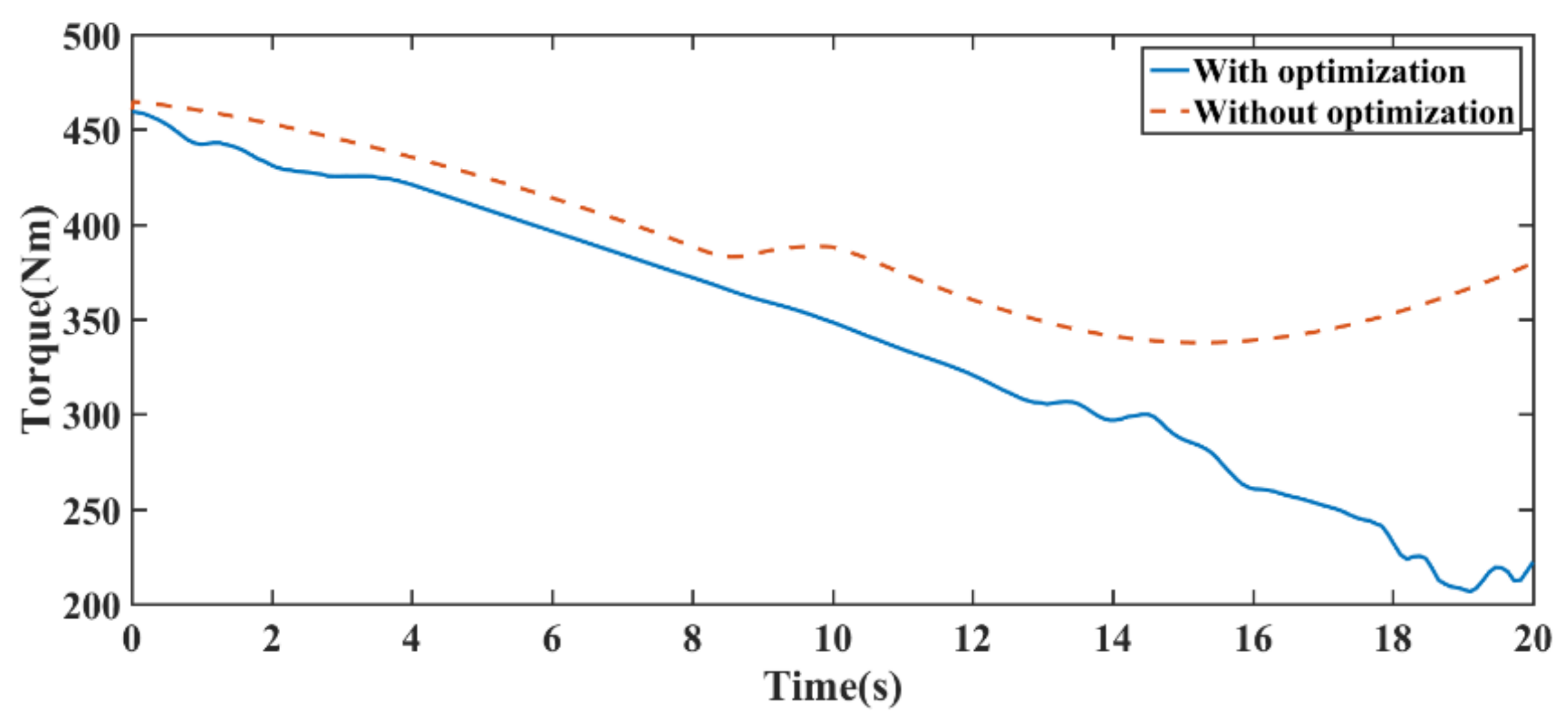
Developing the vibration-reduction trajectory planning algorithm of a mobile redundant manipulator by smoothing the joints’ jerk and minimizing the total torque exerted on the mobile base.

The rest of this paper is organized as follows: Section 2 introduces the kinematic models of the redundant manipulator of the CMBOT. In Section 3, the vibration-reduction motion planning algorithm for CMBOT is proposed. Simulations are conducted to verify the proposed algorithm in Section 4. In addition, Section 5 provides the conclusion. The variables and acronyms in this paper are defined in

Table A1. The description of variables and acronyms.

Variables or Acronyms	Description
Oi	The local coordinate system of each link in manipulator
$\widehat{\mathit{z}}i$	Unit vector of z-axis of Oi
θi	Angle of joint i
αi	Twist angle of link i
δi	Length of link i
di	Offset of link i
${}_{i+1}{}^i\mathit{R}$	Rotation matrix which represents the orientation of Oi+1 with respect to Oi
iωi	Angular velocity and angular acceleration of Oi expressed in Oi
iγi	Angular acceleration of Oi expressed in Oi
iFi	Force acting on the COM of link i
iNi	Torque acting on the COM of link i
$\mathit{M}(\mathit{\theta })$	Mass matrix of the manipulator
$\mathit{C}(\mathit{\theta },\dot{\mathit{\theta }})$	Matrix representing the coefficients of the Coriolis and centrifugal effects
$\mathit{G}(\mathit{\theta })$	Vector accounting for gravity
$\mathit{J}$	Jacobian matrix of the manipulator
${\mathit{J}}^{+}$	Pseudoinverse matrix of J
${}^0\mathit{n}_0$	Torque exerted on the guardrail by the manipulator
VCi	Velocity bound of joint i
ACi	Acceleration bound of joint i
JCi	Jerk bound of joint i
τCi	Torque bound of joint i

.

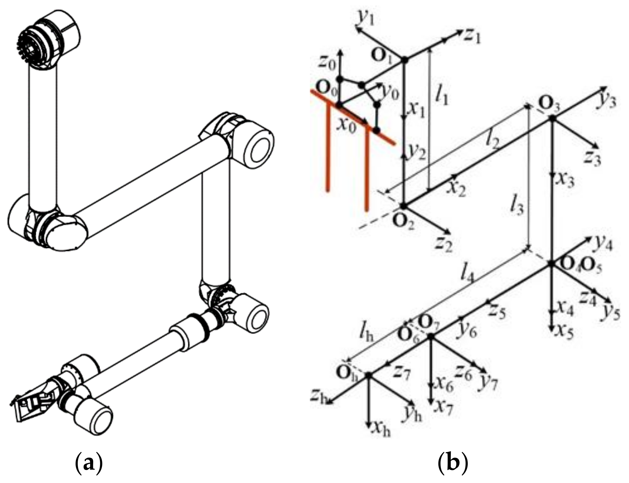
2. Kinematic and Dynamic Modeling of the Outdoor Redundant Manipulator

To reduce casualties during maintenance work on railway bridges, a robot called CMBOT to replace human workers was designed by my team. As shown in Figure 1, the CMBOT consists of a five-degree-of-freedom (5-DOF) biped climbing mechanism with two magnetic feet and a 7-DOF series redundant manipulator. To avoid complex and expensive auxiliary guide rails, the climbing mechanism is designed to climb on the steel bars of the guardrails by using an inchworm-inspired gait and delivering the redundant manipulator to the operating working position. The redundant manipulator then can perform maintenance operations, such as rust removal and spray painting. The working paths of the end effector, which are highlighted by the yellow line in Figure 1a, are all straight lines along the orientation of the structural steel. The prototype of the CMBOT is shown in Figure 1b, the mass of the robot is 68 kg, the maximum length of the redundant manipulator when it is deployed is 2.61 m, and the maximum load of the manipulator is 5 kgs when it is deployed. The workspace of the manipulator can cover a cuboid with the dimensions of 3500 mm × 3500 mm × 1500 mm. The maximum velocity of the biped climbing mechanism along the steel guardrail is 0.03 m/s, the maximum velocity of the end of the manipulator is 0.15 m/s.

A 7-DOF redundant manipulator is selected because the redundant degree of freedom can play an important role in avoiding collisions between the manipulator and obstacles, especially when maintaining the steel brackets under the concrete base. The Denavit-Hartenberg (D-H) method [26] was used to establish the kinematic models of the redundant manipulator. According to the structure diagram in Figure 2a, the coordinate systems of the redundant manipulator are built based on the D-H method, as shown in Figure 2b. The world coordinate system is represented as O₀ and located at the center of the contact surface between the steel guardrail and one of the magnetic feet. The local coordinate system of each link is represented as O_i (i = 1, 2, … 7), and the end-effector coordinate system is defined as O_h. The rotation axis of joint i is set as the z-axis of O_i and its unit vector can be expressed as $\widehat{\mathit{z}}i$. The end-effector is located on the origin of O_h, and its trajectories will be planned based on the demanded operations. l_i (i = 1, 2, 3, 4, h) is the structural parameter of the links. The D-H parameters of the links are shown in

Table 1. D-H parameters of the redundant manipulator.

Link i	Twist Angle αi (°)	Length of Link δi (m)	Offset of Link di (m)	Joint Angle θi/(°)
1	0	0	0	θ1
2	−90	l1 = 0.83	0	θ2
3	0	l2 = 1.00	0	θ3
4	0	l3 = 0.78	0	θ4
5	90	0	l4 = 0.87	θ5
6	−90	0	0	θ6
7	90	0	0	θ7

. Among these D-H parameters, the twist angle, angle range, length of the link and offset of the link are all invariant and are determined by the structure of the redundant manipulator. The joint angle θ_i is the variant that is related to the state of the redundant manipulator. For example, the joint angles of the manipulator shown in Figure 2a are θ₁ = 0°, θ₂ = −90°, θ₃ = 90°, θ₄ = 0°, θ₅ = 0°, θ₆ = 0°, and θ₇ = 0°.

According to the D-H method, the rotation matrix which represents the orientation of O_i+1 with respect to O_i, can be represented as (i = 1, 2, …, 6):

$${}_{i+1}{}^i\mathit{R}=\left[\begin{array}{ccc}\cos \theta i+1& -\sin \theta i+1& 0\\ \sin \theta i+1\cos \alpha i& \cos \theta i+1\cos \alpha i& -\sin \alpha i\\ \sin \theta i+1\sin \alpha i& \cos \theta i+1\sin \alpha i& \cos \alpha i\end{array}\right]$$

(1)

where θ_i is the angle of Joint i and α_i is the twist angle between O_i and O_i+1. The position of the origin of O_i+1 with respect to O_i is defined by (i = 1, 2, …, 6):

$${}^i\mathit{p}_{i+1,1}=\left[\begin{array}{c}ai\\ -sin {\delta }_i d_{i+1}\\ cos {\delta }_i d_{i+1}\end{array}\right]$$

(2)

The vector s = [s_x s_y s_z]^T, which expresses the position of the end-effector relative to O₀, can be represented as the following equation:

$$\mathit{s}={}_1{}^0\mathit{R}{}_2{}^1\mathit{R}{}_3{}^2\mathit{R}{}_4{}^3\mathit{R}{}_5{}^4\mathit{R}{}_6{}^5\mathit{R}{}_7{}^6\mathit{R}{}_h{}^7\mathit{R}{\mathit{s}}_{\mathit{e}}$$

(3)

where s_e = [0 0 l_h]^T is the position of the end-effector relative to the coordinate O₇. If θ = [θ₁ θ₂ θ₃ θ₄ θ₅ θ₆ θ₇]^T is set as the variable parameter of ${}_{i+1}{}^i\mathit{R}$, then Equation (3) can be denoted as s = f(θ).

The dynamic characteristics are also highly important for the motion planning of the manipulator since generalized forces such as joint forces and torques are bound as a result of the physical limits of the actuator. The dynamic parameters for each link are listed in

Table 2. Dynamic parameters for each link.

Link i	Link Mass (kg)	Inertia of Link (Ixx, Iyy, Izz, Ixy, Ixz, Iyz) (kg · m2)	Joint Torque Range (Nm)
1	7.8	(0.02, 0.32, 0.32, 0, −0.01, 0)	±240
2	7.4	(0.04, 0.46, 0.45, −0.01, 0.06, 0)	±240
3	7.7	(0.06, 0.56, 0.59, 0.011, 0.12, 0)	±240
4	4.9	(0.05, 0.03, 0.03, −0.01, 0.01, 0)	±160
5	3.7	(0.25, 0.25, 0.01, 0, 0.01, 0.01)	±160
6	2.5	(0.01, 0.01, 0.003, 0, 0, 0.001)	±160
7	3.62	(0.03, 0.09, 0.07, −0.01, 0.01, 0)	±160

. I_xx, I_yy, I_zz, I_xy, I_xz, and I_yz represent the parameters in the inertia matrix of each link. There are three types of motor drive units used in the redundant manipulator of CMBOT based on its series configuration with the related torque constraints listed in Table 2. Joint 1, joint 2, and joint 3 have the same motor drive units, and the torques are constrained between −240 and 240 Nm. The torques of the other four joints are constrained between −160 and 160 Nm.

The Newton-Euler method, which consists of forward recursion and backward recursion, ${\widehat{\mathit{z}}}_i$ is used to acquire the forces and torques of the links of the manipulator [27]. The center of mass (COM) of the link plays an important role in deciding the dynamic parameters. The accelerations of the COM of the links can be obtained with the following forward recursive algorithm (i = 1, 2, …, 6):

$${}^{i+1}\mathit{\omega }_{+1}={}_{i+1}{}^i\mathit{R}{}^i\mathit{\omega }+{\dot{\theta }}_{i+1}{\widehat{\mathit{z}}}_0$$

(4)

$${}^i\mathit{\gamma }_i={}_{i+1}{}^i\mathit{R}{}^i\mathit{\gamma }_i+{}_{i+1}{}^i\mathit{R}^i{\mathit{\omega }}_i\times {\dot{\theta }}_{i+1}{\widehat{\mathit{z}}}_o+{\ddot{\theta }}_{i+1}{\widehat{\mathit{z}}}_o$$

(5)

$${}^{i+1}\mathit{a}_{i+1}={}_i{}^{i+1}\mathit{R}\left[{}^i\mathit{a}_i+{}^i\mathit{\gamma }_i\times {}^i\mathit{p}_{i+1,1}+{}^i\mathit{\omega }_i\times \left({}^i\mathit{\omega }_i\times {}^i\mathit{p}_{i+1,1}\right)\right]$$

(6)

$${}^{i+1}\mathit{a}_{ci+1}{}^{i+1}\mathit{a}_{i+1}+{}^i\mathit{\gamma }_i\times {}^i\mathit{p}_{ci,i}+{}^i\mathit{\omega }_i\times \left({}^i\mathit{\omega }_i\times {}^i\mathit{p}_{ci,i}\right)$$

(7)

where ⁱω_i and ⁱγ_i are the angular velocity and angular acceleration of O_i expressed in O_i, is a unit vector expressed as [0 0 1]^T, ⁱa_i is the linear acceleration of O_i expressed in O_i, ⁱa_ci is the linear acceleration of COM of link i expressed in O_i, ⁱp_ci,i expresses the position of COM link i with respect to O_i.

The force and torque acting on the COM of link i can be obtained by the following recursive backward algorithm (i = 6, 5, …, 1):

$${}^i\mathit{F}_i=m_i{}^i\mathit{a}_{\mathrm{c}i}$$

(8)

$${}^i\mathit{N}_i={}^i\mathit{I}_i{}^i\mathrm{g}_i{}^i\mathit{\omega }_i\times {}^{i}I_i{}^i\mathit{\omega }_i$$

(9)

$${}^i\mathit{f}_i={}_{i+1}{}^i\mathit{R}^{i+1}{\mathit{f}}_{i+1}+{}^i\mathit{F}_i$$

(10)

$${}^i\mathit{n}_i={}_{i+1}{}^i\mathit{R}^{i+1}{\mathit{n}}_{i+1}+{}^i\mathit{p}_{ci,i}\times {}^i\mathit{F}_i+{}^i\mathit{p}_{i+1,i}\times {}_{i+1}{}^i\mathit{R}^{i+1}{\mathit{n}}_{i+1}+{}^i\mathit{N}_i$$

(11)

where m_i is the mass of link i, ⁱF_i is the force acting on the COM of link i, ⁱN_i represents the torque acting on the COM of link i, ⁱI_i represents the inertia matrix of link i, ⁱf_i is defined as the total force exerted on link i by link i − 1, and ⁱn_i is defined as the total torque exerted on link i by link i − 1. The torque exerted on the guardrail by the manipulator can be represented as

$${}^0\mathit{n}_0={}_1{}^0\mathit{R}{}^1\mathit{n}_1+{}^0\mathit{p}_{0,1}\times {}_1{}^0\mathit{R}{}^1\mathit{f}_1$$

(12)

where ${}_1{}^0\mathit{R}$ is a constant matrix and ${}^0\mathit{p}_{0,1}$ is a constant vector since the position of O₁ related O₁ remains unchanged during the operation of the manipulator.

The torque exerted on joint i of the manipulator can be expressed by the following equation:

$${\mathit{\tau }}_i={}^i\mathit{n}_i{\widehat{\mathit{z}}}_0$$

(13)

Based on Equation (13), the joint torques of the manipulator can also be converted to another expression:

$$\mathit{\tau }=\mathit{M}(\mathit{\theta })\ddot{\mathit{\theta }}+\mathit{C}(\mathit{\theta },\dot{\mathit{\theta }})\dot{\mathit{\theta }}+\mathit{G}(\mathit{\theta })$$

(14)

where τ = [τ₁ τ₂ τ₃ τ₄ τ₅ τ₆ τ₇]^T denotes the joint torques of the manipulator, denotes the angular velocities of the joint and $\ddot{\mathit{\theta }}$ denotes the accelerations of the joints. $\mathit{M}(\mathit{\theta })\in {\mathrm{R}}^{7\times 7}$ is the mass matrix of the manipulator, $\mathit{C}(\mathit{\theta },\dot{\mathit{\theta }})\in {\mathrm{R}}^{7\times 7}$ is the matrix representing the coefficients of the Coriolis and centrifugal effects, and $\mathit{G}(\mathit{\theta })\in {\mathrm{R}}^{7\times 7}$ represents the vector accounting for gravity. The viscous and static friction terms have been neglected for simplicity.

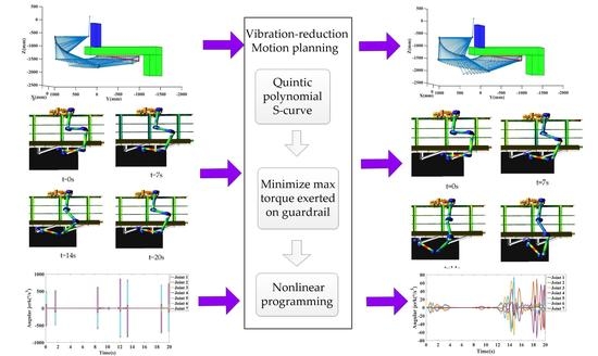
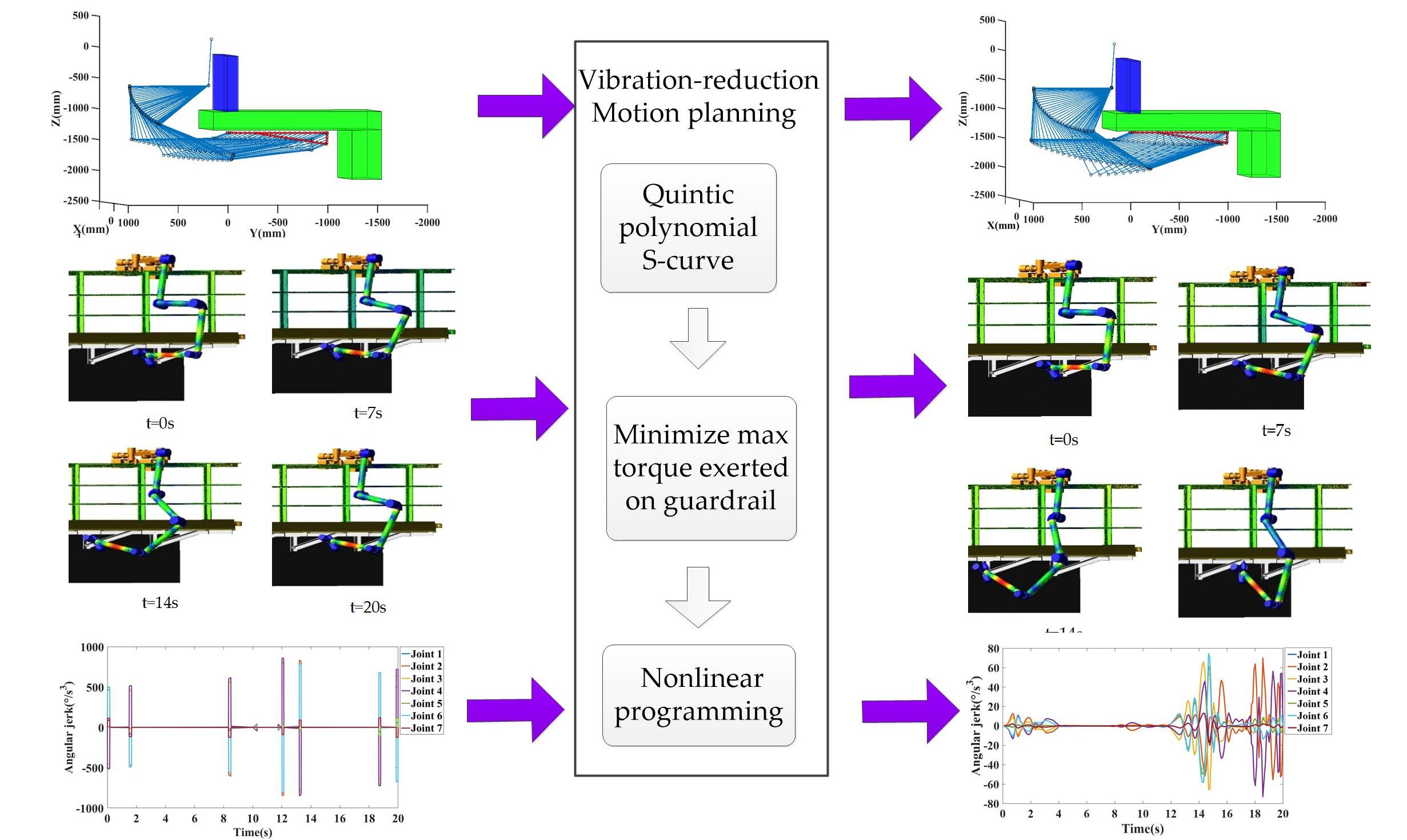
3. Vibration-Reduction Motion Planning Algorithm for the Redundant Manipulator of COMBOT

Utilizing guardrails as guide rails conveniently allows the wide application of CMBOTs, but the poor rigidity of guardrails can also have adverse effects on robot operation. Under the torque exerted by the manipulator, the elastic deformation of the guardrail can cause obvious vibration at the end effector of the redundant manipulator. In addition, the discontinuous trajectories of joints will also induce vibration since the redundant manipulator has four long links that are made of aluminum. Therefore, minimizing the torque exerted by the manipulator on the guardrail and smoothing the trajectories of joints can effectively reduce the vibration of the end effector. To ensure the smoothness of the trajectories, piecewise quintic polynomials are used to interpolate the angular knots of joints that are transformed from the via-points in the obstacle avoidance path. The parameters of the quintic polynomial S-curve are determined by a nonlinear programming problem in which the objective function is to minimize the maximus of the torque exerted by the manipulator on the guardrail throughout the jerk-continuous trajectory. The flowchart of the proposed vibration-reduction motion planning algorithm is illustrated in Figure 3. The innovation of the proposed algorithm is to solve the obstacle avoidance and vibration-reduction problems of the manipulator in motion planning by using nonlinear optimization.

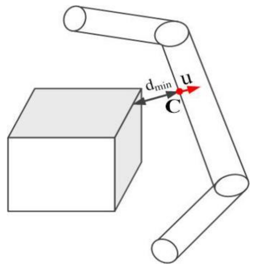
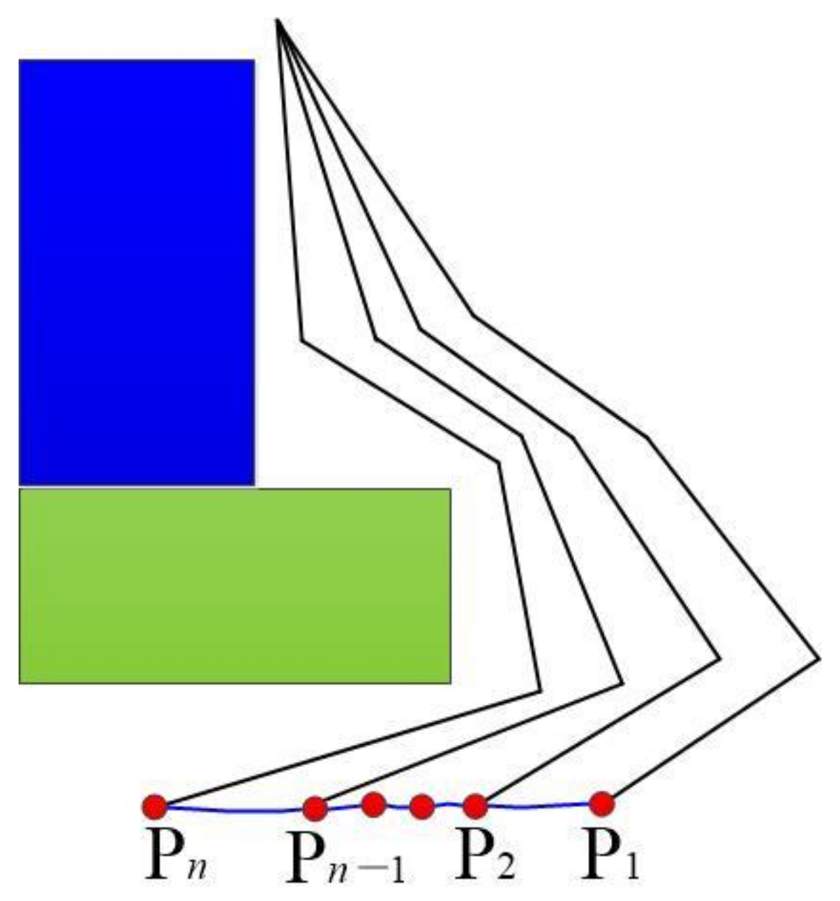
3.1. Collision-Free Geometric Path Planning Based on the Gradient Method with A Singularity-Robust Inverse

To obtain the angular knots of joints in joint space which is the initial condition of a piecewise quintic polynomial trajectory, the predefined working path of the redundant manipulator is needed. To obtain a collision-free working path, the gradient projection method with a singularity-robust inverse is used in this paper. According to the mathematical model of the robotic manipulator, the generalized velocity of the end-effector and the joint angular velocity can be connected as

v = J · θ,

(15)

where v contains the linear velocity and angular velocity along the three axes of O₀. $\mathit{J}\in {\mathrm{R}}^{6\times 7}$ represents the Jacobian matrix of the manipulator. The Jacobian matrix J is calculated according to reference [24]. The general solution of β is denoted by the following equation:

$$\dot{\mathit{\theta }}={\mathit{J}}^{+}\mathit{v}+\beta (\mathit{I}-{\mathit{J}}^{+}\mathit{J})\nabla \mathit{H}$$

(16)

where ${\mathit{J}}^{+}\in {\mathrm{R}}^{7\times 7}$ is the pseudoinverse matrix of J and can be calculated as ${\mathit{J}}^{+}={\mathit{J}}^{\mathrm{T}}{(\mathit{J}{\mathit{J}}^{\mathrm{T}})}^{-1}$. ${\mathit{J}}^{+}\mathit{v}$ is the minimum norm solution of $\dot{\mathit{\theta }}$, which can guarantee that the end-effector tracks the planned trajectory with a minimum sum of the squares of the angular velocities. $\beta (\mathit{I}-{\mathit{J}}^{+}\mathit{J})\nabla \mathit{H}$ is the projection of $\nabla \mathit{H}$, which is located in the zero space of $(\mathit{I}-{\mathit{J}}^{+}\mathit{J})$, and can be regarded as the homogeneous term of $\dot{\mathit{\theta }}$. The homogeneous term can adjust the configuration of the manipulator to meet special demands under the premise of an unchanged trajectory. Among the homogeneous terms, $\nabla \mathit{H}$ denotes the gradient of the optimization index H. β denotes the nonzero optimization coefficient and determines the optimization direction of $\nabla \mathit{H}$. $\mathit{I}\in {\mathrm{R}}^{7\times 7}$ is the identity matrix. If β > 0, a result with a maximum value of H will be obtained, and if β < 0, a result with a minimum value of $\nabla \mathit{H}$ will be obtained.

The risk of collision will increase significantly if the minimum distance between the manipulator and obstacles is less than some given safety threshold. The minimum distance should be increased as much as possible to avoid a collision. Thus, the minimum distance can be regarded as the optimization index H. To maximize the minimum distance, the gradient of the optimization index $\nabla \mathit{H}$ should be in the direction that causes the manipulator to move away from the obstacles at the fastest velocity.

It is highly difficult to calculate this minimum distance since the surfaces of the manipulator and obstacles are irregular. To reduce the computing complexity, the manipulator is simplified as a set of yellow cylinders that can cover all of its own surfaces. The parts of the railway bridge are simplified as a set of blue or green cuboids as obstacles. The appearance of the simplified manipulator and railway bridge is represented in Figure 4.

The minimum distance between typical convex shapes such as cylinders and cuboids can be obtained by the Gilbert-Johnson-Keerthi (GJK) algorithm [28]. The minimum distance between the virtual cylinders and the virtual cuboids is denoted by d_min, and the unit direction vector that points from the closest point in virtual cuboids to the closest point C in virtual cylinders is denoted by u. Figure 5 clearly shows that u is the unit gradient direction that causes d_min increase at the fastest rate.

Let d_s represent the safety threshold between the manipulator and obstacles. Then, the in this paper can be set as the following equation:

$$\nabla \mathit{H}=\left\{\begin{array}{cc}{\mathit{J}}_{\mathrm{C}}^{+}{\mathit{u}}_{\mathrm{m}\mathrm{i}\mathrm{n}},& d_{\mathrm{m}\mathrm{i}\mathrm{n}}\le d_{\mathrm{s}}\\ 0,& d_{\mathrm{m}\mathrm{i}\mathrm{n}}>d_{\mathrm{s}}\end{array}\right.$$

(17)

where ${\mathit{J}}_{\mathrm{C}}^{+}$ is the pseudoinverse Jacobian matrix of point C, which is expressed in O₀. The gradient projection method will produce a smooth path but suffers from the high joint velocities in the vicinity of the singular configurations. The singularity-robust inverse is introduced and merged with the gradient projection method to address this problem. The singular value matrix, which can identify whether the manipulator is in a singular position, can be obtained by UDV decomposition [29]:

$$\mathit{J}=\mathit{U}\mathit{D}{\mathit{V}}^{\mathrm{T}}$$

(18)

where $\mathit{U}\in {\mathrm{R}}^{6\times 6}$, $\mathit{V}\in {\mathrm{R}}^{7\times 7}$ are the orthogonal matrices and $\mathit{D}\in {\mathrm{R}}^{6\times 7}$ is the diagonal matrix whose values consist of the singular values of J and can be denoted as

$$\mathit{D}=\left[\begin{array}{ccccc}{\sigma }_1& 0& ·& ·& 0\\ 0& {\sigma }_2& 0& ·& 0\\ ·& ·& ·& ·& ·\\ 0& ·& 0& {\sigma }_6& 0\end{array}\right]$$

(19)

where σ₁, σ₂, …, σ₆ are the singular values of J and meet the inequality that σ₁ ≥ σ₂ ≥⋯σ₆. σ₆ is the minimum singular value. If σ₆ is close to 0, the manipulator will be in a singular position. In such a situation, the damping coefficient λ will be introduced in the singularity-robust inverse by the following equation:

$${\mathit{J}}^{*}={\mathit{J}}^{\mathrm{T}}{(\mathit{J}{\mathit{J}}^{\mathrm{T}}+{\lambda }^2\mathit{I})}^{-1}$$

(20)

where ${\mathit{J}}^{*}$ is the singularity-robust inverse of J and $\mathit{I}\in {\mathrm{R}}^{7\times 7}$ is the identity matrix. The term ${\lambda }^2\mathit{I}$ can prevent the manipulator from approaching a singular position but introduces extra errors into the results. To reduce these unnecessary errors, the damping coefficient λ will be adjusted according to the value of σ6 using the following equation:

$$\lambda =\left\{\begin{array}{cc}{\lambda }_0\left(1-\frac{{\sigma }_6}{{\sigma }_{\mathrm{h}}}\right),& {\sigma }_6<{\sigma }_{\mathrm{h}}\\ 0,& {\sigma }_6\ge {\sigma }_{\mathrm{h}}\end{array}\right.$$

(21)

where ${\lambda }_0$ is the maximum damping coefficient and σ_h is the threshold of the minimum singular value σ₆. Equation (20) shows that if σ₆ < σ_h, λ will decrease with the increase of σ₆. When σ₆ ≥ σ_h, λ will become 0 since there is no risk for the manipulator to approach a singular position.

If the pseudoinverse matrix J⁺ is replaced with the singularity-robust inverse ${\mathit{J}}^{*}$, the general solution of $\dot{\mathit{\theta }}$ can be rewritten as

$$\dot{\mathit{\theta }}={\mathit{J}}^{\mathrm{T}}{(\mathit{J}{\mathit{J}}^{\mathrm{T}}+{\lambda }^2\mathit{I})}^{-1}\mathit{v}+\beta (\mathit{I}-{\mathit{J}}^{+}\mathit{J})\nabla \mathit{H}$$

(22)

If the optimization coefficient K is set as a positive number, the joint angular velocity that can maximize the minimum distance between the manipulator and obstacle can be obtained to avoid the singularity configuration according to Equation (22). It should be emphasized that, similar to the other existing sample-based planners, the proposed algorithm can also fail to produce a collision-free trajectory when the manipulator is not located at an appropriate position. The algorithm can be regarded as a failed motion planning if the value of d_min is close to 0. In that case, the manipulator should change its initial position and implement the proposed algorithm once more until the trajectory is collision-free.

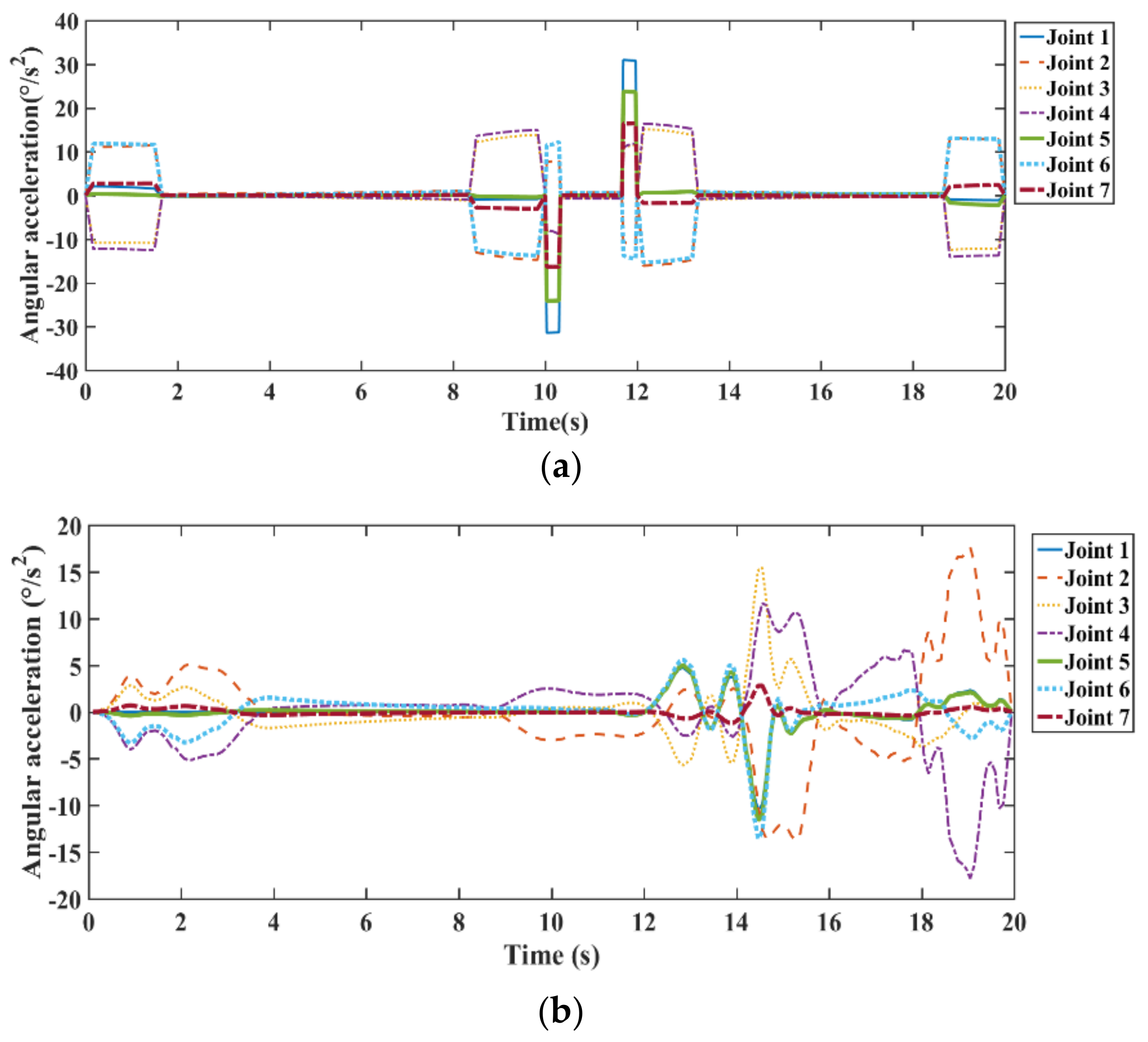
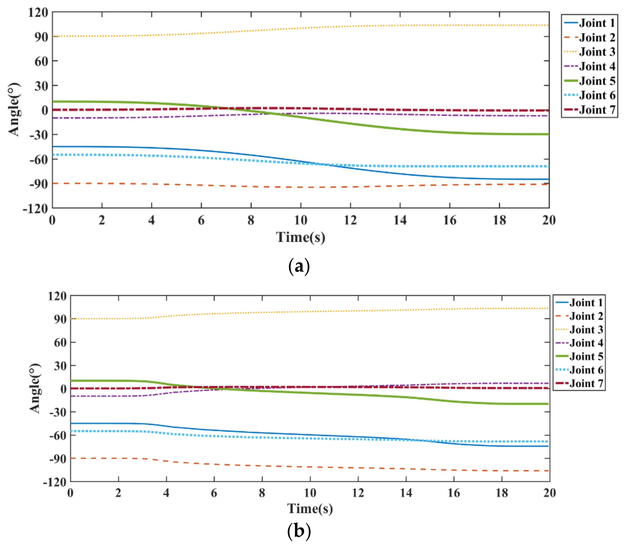
3.2. A Smooth and Vibration-Reduction Trajectory Planning Based on Nonlinear Programming

The joint angles θ can be obtained by the time integration of $\dot{q}$, and the collision-free path can be represented by s = f(θ) according to Equation (3). However, the trajectory obtained through Equation (22) is not smooth since the singularity-robust inverse ${\mathit{J}}^{*}$ cannot vary continuously. To smooth the trajectory and minimize the torque exerted by the manipulator on the guardrail, the joint angular velocities should be replanned to interpolate the sequence of key via-points located on the collision-free paths.

The via-points of the collision-free path, which marked as P_j (j = 1, 2, …, n − 1, n), are showed in Figure 6. The basic objective of trajectory planning is to find a smooth and vibration-reduction trajectory through the via-points. If n via-points are obtained, then the collision-free path is discretized into n − 1 segments. Let t₁ < t₂ <…< t_n−1 < t_n be the time sequence and the corresponding time interval is defined as h_j = t_{j + 1} − t_j (j = 1, 2, …, n − 1, n). The total running time of the trajectory can be defined as

$$T={\sum }_{i=1}^{n-1}{h}_j$$

(23)

To guarantee the desired smoothness property of the trajectory, discretized piecewise quintic polynomials are used to interpolate the sequences of via-points. The trajectory function of the i-th (i = 1, 2, …, 7) joint angle between the j-th segment can be expressed as

$${\theta }_{i,j}\left(t\right)={\displaystyle {\sum }_{k=0}^5{\gamma }_{i,j,k}}{t}^k$$

(24)

where ${\gamma }_{i,j,k}$ is the coefficient of quintic polynomials and k is the serial number of the coefficient. Thus, the corresponding velocity, acceleration, and jerk of joint i relative to the j-th segment can be represented as

$${\dot{\theta }}_{i,j}\left(t\right)={\displaystyle {\sum }_{k=0}^4\left(k+1\right){\gamma }_{i,j,k+1}}{t}^k$$

(25)

$${\ddot{\theta }}_{i,j}\left(t\right)={\displaystyle {\sum }_{k=0}^3\left(k+1\right)\left(k+2\right){\gamma }_{i,j,k+2}}{t}^k$$

(26)

$${\stackrel{\dots }{\theta }}_{i,j}\left(t\right)={\displaystyle {\sum }_{k=0}^2\left(k+1\right)\left(k+2\right)\left(k+3\right){\gamma }_{i,j,k+3}}{t}^k$$

(27)

Equation (27) shows that the jerk function is quadratic polynomials and can guarantee C2 continuity relative to time. To ensure the smoothness of the whole trajectory, the position, velocity, and jerk of the endpoint of the j-th segment must have the same values as the starting point of the j + 1-th segment. Thus, Equations (24) and (25) can be converted to the following equation:

$$\left[\begin{array}{cccccc}1& 0& 0& 0& 0& 0\\ 0& 1& 0& 0& 0& 0\\ 0& 0& 2& 0& 0& 0\\ 1& t_{j+1}& t_{j+1}^2& t_{j+1}^3& t_{j+1}^4& t_{j+1}^5\\ 0& 1& 2t_{j+1}& 3t_{j+1}^2& 4t_{j+1}^3& 5t_{j+1}^4\\ 0& 0& 2& 6t_{j+1}& 12t_{j+1}^2& 20t_{j+1}^3\end{array}\right]\left[\begin{array}{c}{\gamma }_{i,j,0}\\ {\gamma }_{i,j,1}\\ {\gamma }_{i,j,2}\\ {\gamma }_{i,j,3}\\ {\gamma }_{i,j,4}\\ {\gamma }_{i,j,5}\end{array}\right]=\left[\begin{array}{c}{\theta }_{i,j}\left(t_j\right)\\ {\dot{\theta }}_{i,j}\left(t_j\right)\\ {\ddot{\theta }}_{i,j}\left(t_j\right)\\ {\theta }_{i,j}\left(t_{j+1}\right)\\ {\dot{\theta }}_{i,j+1}\left(t_{j+1}\right)\\ {\ddot{\theta }}_{i,j+1}\left(t_{j+1}\right)\end{array}\right]$$

(28)

Taking the coefficients of quintic polynomials as variables, then the coefficients of quintic polynomials can be solved by the matrix inverse operation by Equation (28):

$$\left\{\begin{array}{c}{\gamma }_{i,j,0}={\theta }_{i,j}\left(t_j\right)\\ {\gamma }_{i,j,1}={\dot{\theta }}_{i,j}\left(t_j\right)\\ {\gamma }_{i,j,2}=\frac{{\ddot{\theta }}_{i,j}\left(t_j\right)}{2}\\ {\gamma }_{i,j,3}=\frac{20\left({\theta }_{i,j+1}\left(t_{j+1}\right)-{\theta }_{i,j}(t_j\right)-\left(12{\dot{\theta }}_{i,j}\left(t_j\right)+8{\dot{\theta }}_{i,j+1}\left(t_{j+1}\right)\right)h_j-\left(3{\ddot{\theta }}_{i,j}\left(t_j\right)-{\ddot{\theta }}_{i,j+1}\left(t_{j+1}\right)\right)h_j^2}{2h_j^3}\\ {\gamma }_{i,j,4}=\frac{30\left({\theta }_{i,j}\left(t_j\right)-{\theta }_{i,j+}\left(t_{j+1}\right)\right)+\left(16{\dot{\theta }}_{i,j}\left(t_j\right)+14{\dot{\theta }}_{i,j+1}\left(t_{j+1}\right)\right)h_j-\left(3{\ddot{\theta }}_{i,j}\left(t_j\right)+2{\ddot{\theta }}_{i,j+1}\left(t_{j+1}\right)\right)h_j^2}{2h_j^4}\\ {\gamma }_{i,j,5}=\frac{12\left({\theta }_{i,j+1}\left(t_{j+1}\right)-{\theta }_{i,j}\left(t_j\right)\right)-6\left({\dot{\theta }}_{i,j}\left(t_j\right)+{\dot{\theta }}_{i,j+1}\left(t_{j+1}\right)\right)h_j-\left({\ddot{\theta }}_{i,j}\left(t_j\right)-{\ddot{\theta }}_{i,j+1}\left(t_{j+1}\right)\right)h_j^2}{2h_j^5}\end{array}\right.$$

(29)

where the values of ${\theta }_{i,j}(t_j)$ are determined through via-points of collision-free paths, ${\dot{\theta }}_{i,j}(t_j)$ and ${\ddot{\theta }}_{i,j}(t_j)$ are design variables that are used to optimize the trajectory to minimize the vibration. According to the dynamic analysis of the manipulator, the torque exerted on the guardrail by the manipulator plays an important role in the vibration of the end effector. Thus, the vibration-reduction trajectory planning problem can be formulated as a nonlinear programming problem:

$$\mathrm{m}\mathrm{i}\mathrm{n}\mathrm{i}\mathrm{m}\mathrm{i}\mathrm{z}\mathrm{e} \mathrm{m}\mathrm{a}\mathrm{x}\left|{}^{0}n_0\left(t\right)\right|$$

(30)

$$s.t.\left|\dot{\theta }i,j\left(t\right)\right|\le VCi,\left|\ddot{\theta }i,j\left(t\right)\right|\le ACi,\left|\stackrel{⃛}{\theta }i,j\left(t\right)\right|\le JCi\forall i,j$$

(31)

$$\left|\tau i,j\left(t\right)\right|\le \tau Ci\forall i,j$$

(32)

$$T=TC$$

(33)

$$\dot{\theta }i,j\left(0\right)=\dot{\theta }i,j\left(T\right)=\ddot{\theta }i,j\left(0\right)=\ddot{\theta }i,j\left(T\right)=\stackrel{⃛}{\theta }i,j\left(0\right)=\stackrel{⃛}{\theta }i,j\left(T\right)=0$$

(34)

$$\dot{\theta }i,j\left(tj+1\right)=\dot{\theta }i,j+1\left(tj+1\right)$$

(35)

$$\ddot{\theta }i,j\left(tj+1\right)=\ddot{\theta }i,j+1\left(tj+1\right)$$

(36)

$$\stackrel{⃛}{\theta }i,j\left(tj+1\right)=\stackrel{⃛}{\theta }i,j+1\left(tj+1\right)$$

(37)

where max|⁰n₀(t)| in the objective Function (30) is the maximum torque exerted on the guardrail by the manipulator, and can be calculated by the combination of piecewise quintic polynomial Equations (24)–(29) and the manipulator’s dynamic Equations (4)–(12). Equation (31) includes the kinematics constraints, where VC_i, AC_i, and JC_i are the velocity bound, acceleration bound, and jerk bound of joint i. τC_i in Equation (32) represents the torque bound of joint i, and τ_i,j(t) can be calculated based on Equation (13). TC in Equation (33) is the total running time set by the operator to guarantee the efficiency and productivity of the operation. Equation (34) contains the initial and ultimate time constraints and can avoid abrupt changes at the start or endpoints of the trajectory. The Equations (35)–(37) are continuity constraints that can ensure the seamless connection between adjacent quintic polynomial curves. The sequential quadratic programming algorithm is used to solve the large scales nonlinear programming problem presented above.

4. Simulation and Experiments

To validate the performance of the proposed motion planning algorithm, two typical working paths (the triangular working path along the steel brackets, and the linear working path along the vertical angle steel of guardrails) were simulated and analyzed. The joint torque constraints in Equation (32) are shown in Table 2. The necessary kinematic constraints of the joints which are needed in Equation (31) are listed in

Table 3. Necessary kinematic and dynamic constraints of joints.

Constraint Parameters	Joint 1	Joint 2	Joint 3	Joint 4	Joint 5	Joint 6	Joint 7
VCi (°/s)	20	20	20	30	30	30	30
ACi (°/s2)	60	60	60	90	90	90	90
JCi (°/s3)	160	160	160	240	240	240	240
$\tau Ci$ (Nm)	240	240	240	160	160	160	160

. The results of the collision-free geometric path planning method without vibration-reduction optimization (Equations (15)–(22)) were also presented for comparative study. To solve the nonlinear programming illustrated by Equations (30)–(37), the computing software MATLAB (version R2016a) is used in this paper. The number of via-points n is set as 50 in both two working paths. Many efficient and reliable optimization algorithms have been integrated in MATLAB, and the sequential quadratic programming algorithm is selected to address the proposed nonlinear programming. The maximum number of iterations in this sequential quadratic programming algorithm is set as 1000. The joint velocities of the two planning methods obtained by MATLAB will be sent to drive the rigid-flexible coupling dynamic simulation models built by the dynamic simulation software ADAMS (version 2020) and finite element analysis software ANSYS (version 18.0). The tracking errors of the end effector in the simulations are used to evaluate the effect of the proposed vibration-reduction optimization algorithm.

4.1. Triangle Working Path along the Steel Brackets

As shown in Figure 1, the steel brackets are the most difficult parts to maintain, and the workers have to hang on the guardrail by special equipment to get closer to the steel brackets, which are tens of meters above the ground. Some accidents have occurred during these maintenance operations. The main intention of CMBOT design is to replace the use of workers for bracket maintenance. First, the collision-free path must be found through the gradient method. To avoid the singular configuration, the initial angles of the manipulator in the simulation are set as θ₁ = −10°, θ₂ = −90°, θ₃ = 90°, θ₄ = 0°, θ₅ = 10°, θ₆ = 50° and θ₇ = 0°. The lengths of the three sides of the triangle working path shown in Figrue1 are 100 mm, 200 mm, and 830 mm. The running times of the three sides of the triangle are set as 10 s, 2 s, and 8 s. The trapezoidal velocity trajectory, which is widely used among industrial robots, is used as the initial velocity of the end effector. The velocity curve of the end effector is shown in Figure 7.

Outline information about the railway bridge is acquired by the CAD model, which is created by the CAD software Solidworks. After obtaining the trajectory of the end-effector and the CAD model of the railway bridge, the collision-free trajectory without vibration-reduction optimization can be produced according to Equations (15)–(22), and the collision-free trajectory with vibration-reduction optimization can be produced according to Equations (15)–(22) and the nonlinear optimization Equations (30)–(37). The maximum damping coefficient λ₀ was set to 0.5, and the optimization coefficient β was set to 2 in the simulation. A schematic diagram of the collision-free trajectory without vibration-reduction optimization is shown in Figure 8a, and a schematic diagram of the collision-free trajectory with vibration-reduction optimization is shown in Figure 8b. The colored boxes represent the main obstacles, such as the handrails and brackets of the railway bridge. The cluster of blue straight-line segments represents the links of the manipulator and the red curve represents the trajectory of the end-effector. Figure 8 shows that neither the end effector nor the links of the manipulator collide with the obstacles. The links of the manipulator in the path with vibration-reduction optimization have a closer average distance to the guardrail so that the center of mass of the manipulator will have a closer distance to the guardrail, which can significantly reduce the torque exerted on guardrail.

The joint angles, joint angular velocity, joint angular acceleration, and joint angular jerk of the two collision-free trajectories are shown in Figure 9, Figure 10, Figure 11 and Figure 12 respectively. The joint angular velocity and joint angular acceleration are all within the constraints shown in Table 3. It can be seen from Figure 12 that, the joint angular jerk of the trajectory without optimization exceeds the constraint, and can cause undesired damage to the joints of the manipulator. In addition, the abrupt change of the joint angular jerk of the trajectory without optimization can also aggravate the vibration of the end of the redundant manipulator.

The joint torques of the two collision-free trajectories are shown in Figure 13. It can be clearly seen that the joint torques of the trajectory with optimization tend to decrease in absolute value and lead to a lower torque exerted on the guardrail compared to the joint torques of the trajectory without optimization, which are shown in Figure 14. And the maximum difference of torque exerted on the guard between the trajectory without optimization and trajectory without optimization reached 157.2 Nm, and the lower torque exerted on the guard will lead to a smaller vibration amplitude in the trajectory with optimization.

To validate the vibration reduction effect of the proposed algorithm, the joint velocities of the two trajectories are used to drive the dynamic simulation model of COMBOT, which was built by the ADAMS software. To obtain a more realistic vibration effect, the handrail and the links of the redundant manipulator are converted to flexible parts according to their material characteristics by the finite element analysis software ANSYS. The flexible parts are reassembled in ADAMS to turn the COMBOT simulation model into rigid-flexible coupling components. The simulation time in ADAMS is set to 20 s and the simulation interval is set to 0.02 s. The screenshots of the simulation are shown in Figure 15. The color change of the flexible parts in Figure 15 indicates the change in internal force. The configuration of the redundant manipulator in ADAMS is consistent with the schematic diagram in Figure 8.

The tracking errors of the end effector in the simulation are shown in Figure 16. It can be clearly seen that the tracking errors of the trajectory with optimization are smaller than the tracking errors of the trajectory without optimization. The mean deviation and standard deviation of the tracking errors in linear working path simulation are shown in

Table 4. Statistical results of tracking errors in triangle working path simulation.

Statistical Results of Tracking Errors		X-Axis	Y-Axis	Z-Axis
Without optimization	Mean deviation (mm)	−1.22	3.94	−9.23
	Standard deviation (mm)	1.28	3.99	8.22
With optimization	Mean deviation (mm)	−2.44	11.52	−24.48
	Mean deviation (mm)	4.21	16.20	26.78

. It can be calculated from Table 4 that, the absolute value of the mean deviation of the tracking errors of the X-axis, Y-axis, and Z-axis decreased by 50.1%, 65.8%, and 62.3%, respectively, with vibration-reduction optimization. The results indicate that the proposed algorithm can markedly reduce the vibration in the triangle working path.

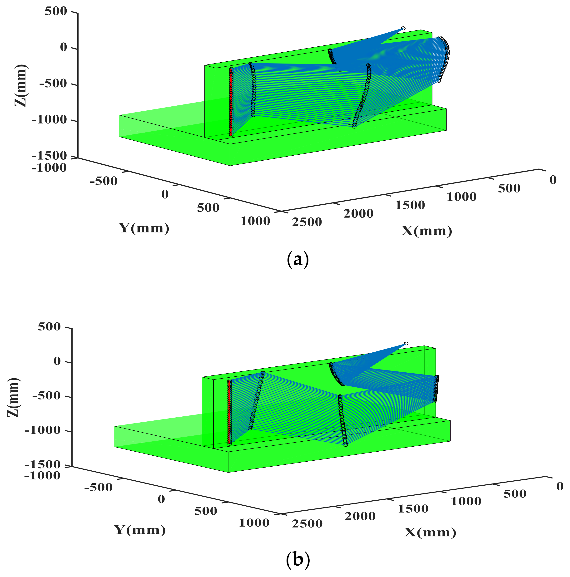
4.2. Linear Working Path along the Vertical Angle Steel of the Guardrails

The linear working path along the vertical angle steel of guardrails is also a common path during maintenance. To avoid the singular configuration, the initial angles of the manipulator in the simulation are set as θ₁ = −45°, θ₂ = −90°, θ₃ = 90°, θ₄ = −10°, θ₅ = 10°, θ₆ = −55° and θ₇ = 0°. The length of the linear working path shown in Figure 1 is 940 mm. The running time of the linear working path is set as 20 s. The initial velocity curve of the end effector based on the trapezoidal velocity trajectory is shown in Figure 17.

After obtaining the trajectory of the end-effector and the CAD model of the railway bridge, collision-free trajectories with and without vibration-reduction optimization can be produced by using MATLAB. The maximum damping coefficient ${\lambda }_0$ was set to 0.5, and the optimization coefficient β was set to 2 in the simulation. A schematic diagram of the collision-free trajectory without vibration-reduction optimization is shown in Figure 18a, and a schematic diagram of the collision-free trajectory with vibration-reduction optimization is shown in Figure 18b. Figure 18 shows that neither the end effector nor the links of the manipulator collide with the obstacles. The links of the manipulator in the path with vibration-reduction optimization have a closer average distance to the guardrail so that the center of mass of the manipulator will have a closer distance to the guardrail, which can significantly reduce the torque exerted on guardrail.

The joint angles, joint angular velocity, joint angular acceleration, and joint angular jerk of the two collision-free trajectories are shown in Figure 19, Figure 20, Figure 21 and Figure 22, respectively. The joint angular velocity, joint angular acceleration, and joint angular jerk are all within the constraints shown in Table 3. It can be seen from Figure 22 that, the joint angular jerk of the trajectory without optimization obviously has an abrupt change which can aggravate the vibration of the end of the redundant manipulator.

The joint torques of the two collision-free trajectories are shown in Figure 23. It can be clearly seen that the joint torques of the trajectory with optimization tend to decrease in absolute value and lead to a lower torque exerted on the guardrail compared to the joint torques of the trajectory without optimization, which are shown in Figure 24. And the maximum difference of torque exerted on the guard between the trajectory without optimization and trajectory without optimization reached 89.14 Nm, and the lower torque exerted on the guard will lead to a smaller vibration amplitude in the trajectory with optimization.

To validate the vibration-reduction effect of the proposed algorithm, the joint velocities of the two trajectories are used to drive the rigid-flexible coupling dynamic simulation model of COMBOT built by ADAMS and ANSYS. The simulation time in ADAMS is set to 20 s and the simulation interval is set to 0.02 s. The screenshots of the simulation are shown in Figure 25. The configuration of the redundant manipulator in ADAMS is consistent with the schematic diagram in Figure 18.

The tracking errors of the end effector in the simulation are shown in Figure 26. It can be clearly seen that the tracking errors of the trajectory with optimization are smaller than the tracking errors of the trajectory without optimization. The mean deviation and standard deviation of the tracking errors in linear working path simulation are shown in

Table 5. Statistical results of tracking errors in linear working path simulation.

Statistical Results of Tracking Errors		X-Axis	Y-Axis	Z-Axis
Without optimization	Mean deviation (mm)	−2.13	−2.03	−2.55
	Standard deviation (mm)	2.01	2.26	3.39
With optimization	Mean deviation (mm)	−6.17	−3.93	−5.36
	Mean deviation (mm)	7.62	4.63	7.87

. It can be calculated from Table 5 that, the absolute value of the mean deviation of the tracking errors of the X-axis, Y-axis, and Z-axis decreased by 65.5%, 48.3%, and 52.4%, respectively, with vibration-reduction optimization. The results indicate that the proposed algorithm can markedly reduce the vibration along the linear working path.

5. Conclusions

To reduce the vibration of the manipulator caused by the discontinuous trajectories of joints and the low rigidity of the guardrail, a motion planning algorithm for vibration reduction is proposed in this paper. A series of comparative simulation experiments are conducted to validate the effectiveness of the proposed vibration-reduction algorithm. The results show that the proposed algorithm can effectively reduce the vibration of the end effector of the manipulator. The vibration-reduction motion planning method contains two parts: On the one hand, the vibration-reduction trajectory tends to shorten the distance between the COM of the redundant manipulator and the guardrail, which can reduce the torque caused by gravity; on the other hand, the smooth and constrained joint angular jerk can reduce the vibration caused by the abrupt change in joint angular acceleration. The efficiency improvement is reflected in the obvious reduction of tracking errors. The average tracking errors of the three coordinate axes decreased by at least 48.3% compared to the trajectory without vibration reduction in the simulation. The outdoor mobile manipulator has more and more broad applications in the fields of building curtain wall cleaning, disaster rescue, bridge maintenance, and so on. The vibration reduction algorithm proposed in this paper helps to reduce the vibration of the outdoor robot with a series structure in the process of motion and improve the trajectory accuracy, which is of great significance to promote the application of outdoor mobile robots.

6. Future Works

The prototype experimental platform of CMBOT has been designed and will be manufactured and assembled in the future. The proposed vibration-reduction algorithm will be tested on the prototype experimental platform. Meanwhile, the vibration of the bridge and the wind pressure caused by the passing train also influence the vibration of the manipulator. The method to reduce the vibration caused by the passing train to extend the continuous working hours of the CMBOT will be studied in the future.

References

1. Dorafshan, S.; Maguire, M. Bridge inspection: Human performance, unmanned aerial systems and automation. J. Civ. Struct. Health Monit. 2018, 8, 443–476. [Google Scholar] [CrossRef] [Green Version]
2. Chu, B.; Jung, K.; Han, C.S.; Hong, D. A survey of climbing robots: Locomotion and adhesion. Int. J. Precis. Eng. Manuf. 2010, 11, 633–647. [Google Scholar] [CrossRef]
3. Huang, H.; Li, D.; Xue, Z.; Chen, X.; Liu, S.; Leng, J.; Wei, Y. Design and performance analysis of a tracked wall-climbing robot for ship inspection in shipbuilding. Ocean Eng. 2017, 131, 224–230. [Google Scholar] [CrossRef]
4. Pagano, D.; Liu, D. An approach for real-time motion planning of an inchworm robot in complex steel bridge environments. Robotica 2017, 35, 1280–1309. [Google Scholar] [CrossRef]
5. Muthugala, M.A.V.J.; Le, A.V.; Cruz, E.S.; Elara, M.R.; Veerajagadheswar, P.; Kumar, M. A self-organizing fuzzy logic classifier for benchmarking robot-aided blasting of ship hulls. Sensors 2020, 20, 3215. [Google Scholar] [CrossRef]
6. Muthugala, M.A.V.J.; Vega-Heredia, M.; Vengadesh, A.; Sriharsha, G.; Elara, M.R. Design of an adhesion-aware façade cleaning robot. In Proceedings of the 2019 IEEE/RSJ International Conference on Intelligent Robots and Systems (IROS), Macau, China, 3–8 November 2019; pp. 1441–1447. [Google Scholar]
7. Eldred, R.; Lussier, J.; Pollman, A. Design and Testing of a Spherical Autonomous Underwater Vehicle for Shipwreck InteriorExploration. J. Mar. Sci. Eng. 2021, 9, 320. [Google Scholar] [CrossRef]
8. Chang, Q.; Luo, X.; Qiao, Z. Design and Motion Planning of a Biped Climbing Robot with Redundant Manipulator. Appl. Sci. 2019, 9, 3009. [Google Scholar] [CrossRef] [Green Version]
9. Lu, S.; Ding, B.; Li, Y. Minimum-jerk trajectory planning pertaining to a translational 3-degree-of-freedom parallel manipulator through piecewise quintic polynomials interpolation. Adv. Mech. Eng. 2020, 12, 1–18. [Google Scholar] [CrossRef]
10. Li, L.; Xiao, J.; Zou, Y. Time-optimal path tracking for robots a numerical integration-like approach combined with an iterative learning algorithm. Ind. Robot. 2019, 46, 763–777. [Google Scholar] [CrossRef]
11. Pham, H.; Pham, Q. A new approach to time-optimal path parameterization based on reachability analysis. IEEE Trans. Robot. 2018, 34, 645–659. [Google Scholar] [CrossRef] [Green Version]
12. Consolini, L.; Locatelli, M.; Minari, A. Optimal time-complexity speed planning for robot manipulators. IEEE Trans. Robot. 2019, 35, 790–797. [Google Scholar] [CrossRef]
13. Verscheure, D.; Demeulenaere, B.; Swevers, J. Time-optimal path tracking for robots: A convex optimization approach. IEEE Trans. Autom. Control. 2009, 54, 2318–2327. [Google Scholar] [CrossRef]
14. Reiter, A.; Müller, A.; Gattringer, H. On higher order inverse kinematics methods in time-optimal trajectory planning for kinematically redundant manipulators. IEEE Trans. Ind. Inform. 2018, 14, 1681–1690. [Google Scholar] [CrossRef]
15. Fang, Y.; Hu, J.; Liu, W. Smooth and time-optimal S-curve trajectory planning for automated robots and machines. Mech. Mach. Theory 2019, 137, 127–153. [Google Scholar] [CrossRef]
16. Brossog, M.; Bornschlegl, M.; Franke, J. Reducing the energy consumption of industrial robots in manufacturing systems. Int. J. Adv. Manuf. Technol. 2015, 78, 1315–1328. [Google Scholar]
17. Sands, T. Optimization provenance of whiplash compensation for flexible space robotics. Aerospace 2019, 6, 93. [Google Scholar] [CrossRef] [Green Version]
18. Saramago, S.; Junior, V. Optimal trajectory planning of robot manipulators in the presence of moving obstacles. Mech. Mach. Theory 2000, 35, 1079–1094. [Google Scholar] [CrossRef]
19. Li, Y.; Huang, T.; Chetwynd, D. An approach for smooth trajectory planning of high-speed pick-and-place parallel robots using quintic B-splines. Mech. Mach. Theory 2018, 126, 479–490. [Google Scholar] [CrossRef] [Green Version]
20. Piazzi, A.; Visioli, A. Global minimum-jerk trajectory planning of robot manipulators. IEEE Trans. Ind. Inform. 2000, 47, 140–149. [Google Scholar] [CrossRef] [Green Version]
21. Macfarlane, S.; Croft, E. Jerk-bounded manipulator trajectory planning: Design for real-time applications. IEEE Trans. Robot. Autom. 2003, 19, 42–52. [Google Scholar] [CrossRef] [Green Version]
22. Gasparetto, A.; Zanotto, V. A technique for time-jerk optimal planning of robot trajectories. Robot. Comput. Integr. Manuf. 2008, 24, 415–426. [Google Scholar] [CrossRef]
23. Gasparetto, A.; Lanzutti, A.; Vidoni, R. Validation of minimum time-jerk algorithms for trajectory planning of industrial robots. J. Mech. Robot. 2011, 3, 031003. [Google Scholar] [CrossRef]
24. Bianco, C. Minimum-jerk velocity planning for mobile robot applications. IEEE Trans. Robot. 2013, 29, 1317–1326. [Google Scholar] [CrossRef]
25. Huang, T.; Wang, P.; Mei, J. Time minimum trajectory planning of a 2-DOF translational parallel robot for pick-and-place operations. CIRP Ann. 2007, 56, 365–368. [Google Scholar] [CrossRef]
26. Rocha, C.; Tonetto, A.; Dias, A. A comparison between the Denavit–Hartenberg and the screw-based methods used in kinematic modeling of robot manipulators. Robot. Comput. Integr. Manuf. 2011, 27, 723–728. [Google Scholar] [CrossRef]
27. Bianco, C. Evaluation of generalized force derivatives by means of a recursive Newton–Euler approach. IEEE Trans. Robot. 2009, 25, 954–959. [Google Scholar] [CrossRef]
28. Gilbert, E.; Johnson, D.; Keerthi, S. A fast procedure for computing the distance between complex objects in three-dimensional space. IEEE Trans. Rob. Autom. 1988, 4, 193–203. [Google Scholar] [CrossRef] [Green Version]
29. Yang, H.; Li, H. Weighted UDV*-decomposition and weighted spectral decomposition for rectangular matrices and their applications. Appl. Math. Comput. 2008, 198, 150–162. [Google Scholar] [CrossRef]
Figure 1. Overall structure of the CMBOT. (a) Sketch of the CMBOT, (b) Prototype of the CMBOT.
Electronics 10 02793 g001
Figure 2. Structure diagram and coordinate systems of the CMBOT. (a) Structure diagram of the redundant manipulator. (b) The coordinate systems based on the D-H method.
Electronics 10 02793 g002
Figure 3. Flowchart of the proposed vibration-reduction motion planning algorithm.
Electronics 10 02793 g003
Figure 4. Manipulator and railway bridges simplified as cylinders and cuboids.
Electronics 10 02793 g004
Figure 5. Minimum distance between virtual cylinders and obstacles.
Electronics 10 02793 g005
Figure 6. Via-points on the collision-free path.
Electronics 10 02793 g006
Figure 7. Velocity curve of the end effector.
Electronics 10 02793 g007
Figure 8. Schematic diagram of the collision-free trajectories of the manipulator. (a) Without optimization, (b) With optimization.
Electronics 10 02793 g008
Figure 9. Joint angles of trajectories. (a) Without optimization, (b) With optimization.
Electronics 10 02793 g009
Figure 10. Joint angular velocity of trajectories. (a) Without optimization, (b) With optimization.
Electronics 10 02793 g010
Figure 11. Joint angular acceleration of trajectories. (a) Without optimization, (b) With optimization.
Electronics 10 02793 g011
Figure 12. Joint angular jerk of trajectories. (a) Without optimization, (b) With optimization.
Electronics 10 02793 g012
Figure 13. Joint torque of trajectories. (a) Without optimization, (b) With optimization.
Electronics 10 02793 g013
Figure 14. Torque exerted on the guardrail by the manipulator.
Electronics 10 02793 g014
Figure 15. Screenshots of the simulation. (a) Without optimization, (b) With optimization.
Electronics 10 02793 g015
Figure 16. The tracking errors of the end effector in simulation. (a) Tracking error of X axis; (b) Tracking error of Y axis; (c) Tracking error of Z axis.
Electronics 10 02793 g016
Figure 17. Velocity curve of the end effector.
Electronics 10 02793 g017
Figure 18. Schematic diagram of the collision-free trajectories of the manipulator. (a) Without optimization, (b) With optimization.
Electronics 10 02793 g018
Figure 19. Joint angles of trajectories. (a) Without optimization, (b) With optimization.
Electronics 10 02793 g019
Figure 20. Joint angular velocity of trajectories. (a) Without optimization, (b) With optimization.
Electronics 10 02793 g020
Figure 21. Joint angular acceleration of trajectories. (a) Without optimization, (b) With optimization.
Electronics 10 02793 g021
Figure 22. Joint angular jerk of trajectories. (a) Without optimization, (b) With optimization.
Electronics 10 02793 g022
Figure 23. Joint torque of trajectories. (a) Without optimization, (b) With optimization.
Electronics 10 02793 g023
Figure 24. Torque exerted on the guardrail by the manipulator.
Electronics 10 02793 g024
Figure 25. Screenshots of the simulation. (a) Without optimization, (b) With optimization.
Electronics 10 02793 g025
Figure 26. The tracking errors of the end effector in simulation. (a) Tracking error of X axis; (b) Tracking error of Y axis; (c) Tracking error of X axis.
Electronics 10 02793 g026