Precision Fibre Angle Inspection for Carbon Fibre Composite Structures Using Polarisation Vision

Abstract

This paper evaluates the precision of polarisation imaging technology for the inspection of carbon fibre composite components. Specifically, it assesses the feasibility of the technology for fibre orientation measurements based on the premise that light is polarised by reflection from such anisotropically conductive surfaces. A recently commercialised Sony IMX250MZR sensor is used for data capture by using various lighting conditions. The paper shows that it is possible to obtain sub-degree accuracy for cured and dry woven and unidirectional materials in ideal conditions, which comprised dark field illumination. Indeed, in ideal conditions, the average relative angles can be measured to an accuracy of 0.1–0.2°. The results also demonstrate a precision of the order 1° for more general illumination, such as dome illumination and ambient lighting, for certain material type/lens combinations. However, it is also shown that the precision varies considerably depending on illumination, lens choice and material type, with some results having errors above 2°. Finally, a feasibility study into the inspection of three-dimensional components suggests that only limited application is possible for non-planar regions without further research. Nevertheless, the observed phenomena for such components are, at least, qualitatively understood based on physics theory.

1. Introduction

The use of composite structures in various industries has increased in recent decades due to their advantages over conventional materials. Most notably, carbon fibre reinforced polymer (CFRP) components offer exceptionally high strength-to-weight ratios and are, thus, highly attractive for aerospace engineering. Other advantages of CFRP include high stiffness, corrosion resistance and low thermal expansion. Consequently, CFRP usage is becoming increasingly popular in other areas such as maritime, civil and automotive engineering [1].

Due to this increased use of CFRP—in addition to its higher manufacturing costs—the need for inspection and repair technologies for such materials has increased accordingly. This is particularly important since the strength and stiffness of composite parts are highly dependent on the placement and orientation of fibres during manufacture [2]: a 5° angular error in orientation, for example, can result in a 20% reduction in component strength [3]. Due to this importance and the time consuming nature of inspection, a great deal of resources are often devoted to the inspection of parts. Rudberg et al., for example, stated that 33% of the time taken for automated fibre placement in aerostructures can be devoted to inspection and repair [4]. Therefore, precise measurement of fibre orientation plays an important role during manufacturing quality assurance.

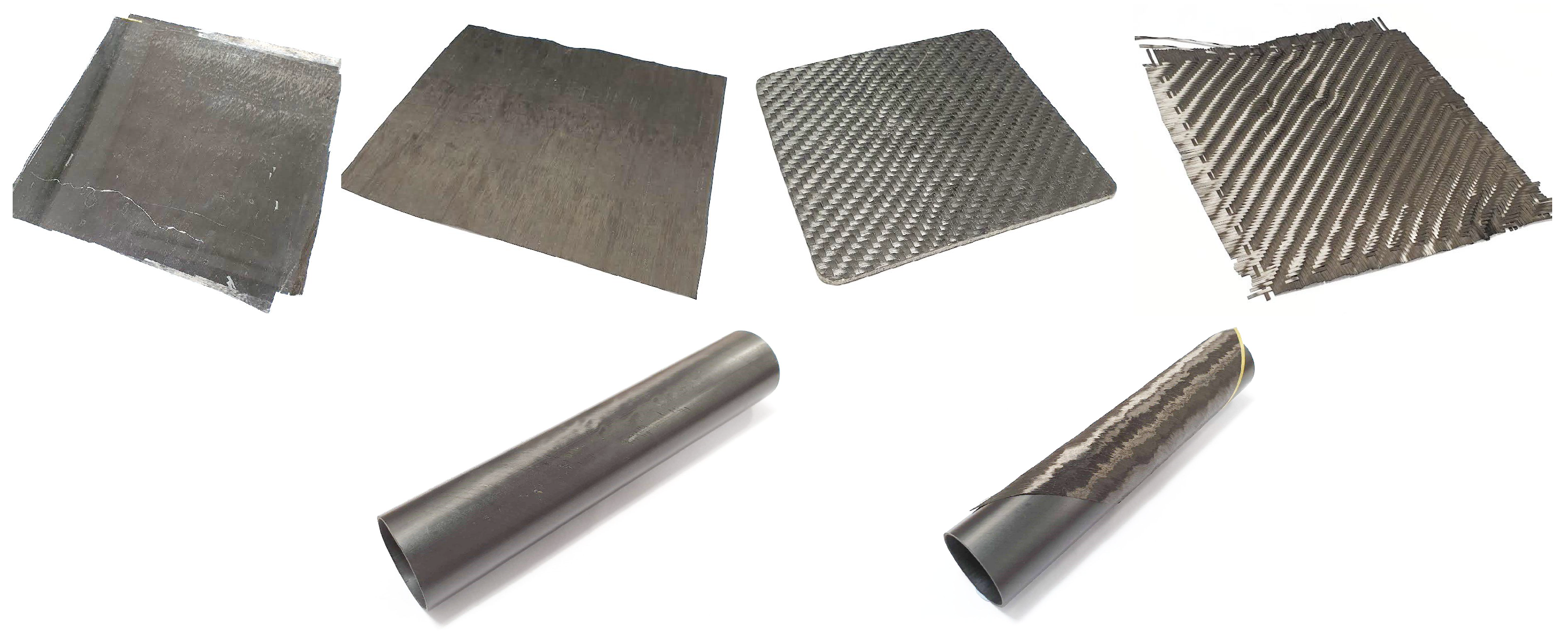
Motivated by the above, the aim of this paper is to assess the accuracy and reliability of an emerging non-destructive technology used for the analysis of composite parts: polarisation vision. Specifically, the paper presents research into the feasibility of this technology for widespread adoption in the field with a primary focus on fibre orientation measurement of carbon fibre materials. The paper considers both dry materials (i.e., raw and untreated carbon fibre fabrics) and cured materials (those with the fibres set in resin, forming a hardened composite part). It should be noted that only minor changes to the presented method would be required to make the inspection more general (e.g., to localise specific defects such as waviness or fuzzballs) since many such defects manifest as local unexpected variations in fibre angle. Only carbon fibres are considered here since other types, such as glass fibres, do not possess the requisite anisotropic conductivity for the appropriate theory (Section 2.1) to apply.

Polarisation vision is a growing sub-field of computer vision that uses polarisation data to extract useful information about a scene or object. It can be defined as “the acquisition and use of images that encode information about the polarisation state of incoming light” [5]. Images captured with this technology typically encode polarisation data in a three channel image, where each channel contains the following information [5]:

• Intensity, I: Identical to a standard monochrome image;
• Phase or angle of linear polarisation (AoLP), $\varphi$: Angle of polarisation of incoming light at each pixel;
• Degree of polarisation (DoP), ρ: Fraction of the incoming light that is polarised at each pixel, ranging from 0 (unpolarised) to 1 (completely linearly polarised).

This paper primarily uses the AoLP since it aligns with the fibre angles on the surface under investigation, as explained in Section 2.1.

The remainder of this paper is organised as follows. First, a summary of the existing literature in the field is presented followed by a list of the main contributions of this research study. Section 2 then describes the underlying principles of the physics of reflectance used for this research study as well as the hardware used and algorithmic approach to data processing. Section 3 covers the detailed numerical results of the study, demonstrating the levels of precision expected in both ideal and non-ideal conditions. The primary focus is on planar surfaces, although non-planar surfaces are briefly considered in Section 3.3. A discussion of the significance of the research with respect to real application areas is provided in Section 4 before Section 5 concludes the paper.

1.1. Related Work

The following subsections cover existing research in composite part inspection before reviewing polarisation vision hardware and its applications.

1.1.1. Composite Part Inspection

Many non-destructive methods currently exist for quality assurance during manufacturing and damage detection on composite structures. Most of these are highlighted in [6,7], such as acoustics, shearography, thermography, etc. One particularly sophisticated non-destructive method is X-ray computed tomography (CT) as it provides geometrically accurate subsurface imaging of a component [8]. Researchers have exploited this technology to develop an interactive tool for visual analysis of fibre properties on CFRP components [9]. This tool often uses parallel coordinates to define and configure initial fibre classes before applying polar plots to render fibre orientation distributions [9]. Further work on the application of X-ray CT for composite inspection can be found in [10,11]. Nelson et al. highlighted that one disadvantage of the method is that the physical size of typical aerospace components often precludes inspection using X-ray CT methods because spatial resolution requirements cannot be achieved [8]. However, spatial resolution is improving and different strategies can be adopted to overcome sample size/resolution issues [12]. Certainly, CT scanners remain expensive and unwieldy.

Another dominant non-destructive method for composite inspection is ultrasound. Pulse-echo ultrasound is commonly used in aerospace for analysis of large composite components; however, data generated from the technique do not intuitively reveal ply and fibre features [8]. Nelson et al. demonstrate that ultrasonic instantaneous-phase data can be analysed by using image processing algorithms to produce three-dimensional maps of ply orientations [8]. Unfortunately, the researchers concluded that further work was necessary to produce robust measurements.

Computer vision methods for inspection have proved challenging on CFRP surfaces due to their black and shiny nature. Several attempts have been proposed based on traditional image processing and edge detection, but these inherently need very high quality and high resolution images that are not always tractable [13,14]. Furthermore, the methods were not proven on materials with plain appearance such as unidirectional surfaces with no visible stitching. In order to overcome the difficult reflectance properties, Zambal et al. [15] used a specialised lighting rig and modelled the reflectance properties of fibres to determine their orientations. This provided sub-degree precision for more general CFRP surfaces at the expense of longer capture times and the need for highly controlled illumination.

Recently, polarisation vision has been applied to the analysis of carbon fibre composite structures since the anisotropic conductance of such materials means that the angle of polarisation of reflected light matches the fibre orientation of each point on a surface [16,17]. The key elements demonstrated from these works are as follows:

• The angle of linear polarisation corresponds to the angle of orientation of the fibres (both dry and cured), as predicted by the underlying physics theory.
• Reflection from CFRP materials causes unpolarised incident light to become partially polarised. As such, an unpolarised light source is sufficient for data capture.
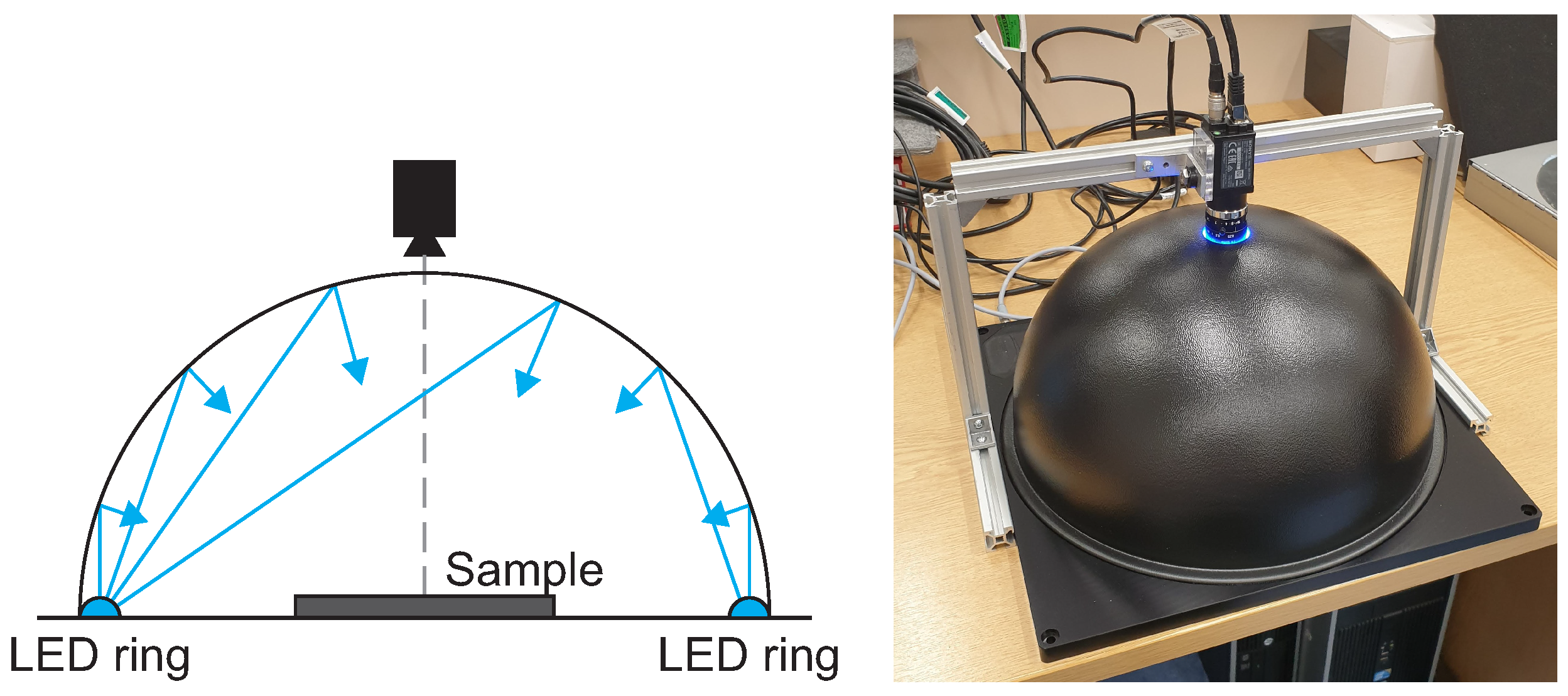
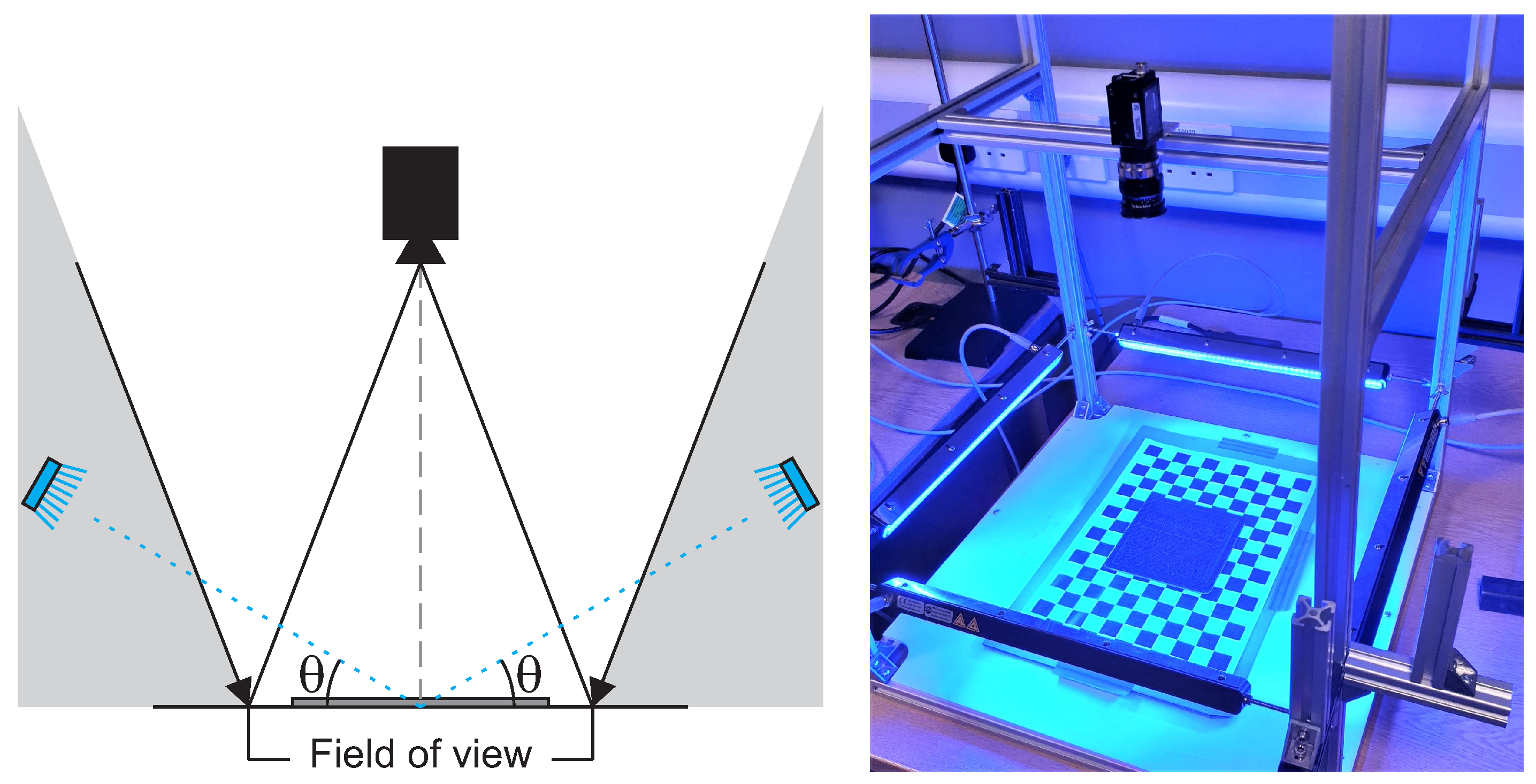
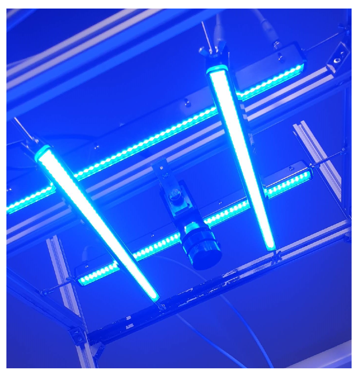
• Light intensity and distribution are important factors to consider as some illuminations will result in no light being reflected from certain fibres. A dome illumination can be used for ensuring uniform illumination throughout the entire component.
• The degree of polarisation shows the amount of polarised vs. unpolarised light, which can add confidence levels to individual measurements.

Further studies on the application of polarisation vision for composite part inspection can be found in [18] where Atkinson et al. first focused on demonstrating the ability of polarisation technology for image recovery on diffuse, non-fibrous surfaces before performing a brief test on a planar CFRP sample. The results gathered from the experiments in [18] highlight that the fibre orientation distribution corresponds to the angle of linear polarisation, as stated in [16], and that the AoLP histogram allows for the determination of the main angles present. The pros and cons of polarisation compared to alternative methods are summarised in

Table 1. Pros and cons of polarisation vision for CFRP inspection compared to alternative technologies.

Compared to Non-Vision Methods
Pros	Cons
Financially inexpensive	Only inspects top exposed layer
Small footprint	Unreliable for glass fibres
Easier to install on production line
Typically higher resolution
Uses less power
Higher-speed data capture
Compared to Other Computer Vision Methods
Pros	Cons
More robust to poor illumination	Slightly more expensive camera
Not reliant on stitching etc.	Resolution limited due to special camera
General layup structure/curing status

.

1.1.2. Polarisation Vision Hardware

The field of polarisation vision initially developed in the 1980s with several major contributions from Wolff and coworkers in the 1990s [19,20,21]. Without specialist hardware, polarisation data have been captured by using a standard, typically monochrome, camera with a mechanically rotating linear polarising filter placed in front of the lens. With this method, at least three images are needed at different polariser orientations to obtain a complete measurement of partial linear polarisation [5,21,22]. This assumes that there is no circular/elliptical polarisation present. However, due to the need for rotating optics, the measurements of AoLP and DoP are slow and, thus, limited to static scenes.

The development of liquid crystal polarisation cameras opened up further applications as the polariser transmission axis could be switched much more rapidly [23,24]. These “polarisation cameras” then allowed for faster data acquisition as there was no longer a mechanically rotating part. However, captured data were highly susceptible to noise, and capture time was still longer than a standard camera [5]. For these reasons, widespread adoption of the technology was still limited well after the turn of the century.

An alternative approach to data capture was to use a polarising beam splitter that allows for real-time measurements of partial linear polarisation [25,26]. Indeed Pezzaniti et al. were able to recover full Stokes vector parameters at 60 frames per second [26]. While this provides higher frame rates than the above mentioned liquid crystal polarisation cameras, this comes as a trade-off as such an arrangement is expensive and difficult to calibrate [5].

Since the development of the above capture methods, many cameras have emerged that overcome some of their issues by incorporating polarising filters directly onto the sensor chip [17,27,28]. One of the earliest, the “POLKA”, was developed at the Fraunhofer Institute for Integrated Circuits and is compared to the rotating filter method in [5], showing comparable precision but at much faster frame rates. 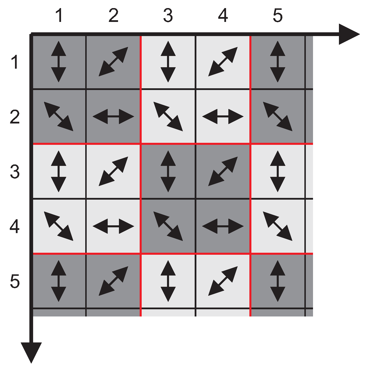The POLKA was also used in early efforts for determining strand orientation in CFRP components for contactless quality inspection [16]. This is even demonstrated on moving parts. This paper uses a similar sensor to POLKA, the Sony IMX250MZR. Similarly to the POLKA, the Sony sensor uses monochrome quad-polarised filters to capture polarised light in four planes [29], as detailed in Section 2.2.

1.1.3. Other Polarisation Vision Applications

Perhaps the most widely studied application for polarisation vision in computer vision literature is three-dimensional shape analysis [19,22,30,31] where polarisation information is used to estimate the geometry of an object. In 2004, Atkinson et al. applied the Fresnel theory to recover the shape of an object in diffuse polarisation cases and concluded that diffuse polarisation had potential for such application when combined with other computer vision techniques [22]. Atkinson later, therefore, incorporated binocular [30] and photometric [31] stereo in order to improve precision. Miyazaki et al. [24] used polarisation on transparent surfaces for shape estimation of particularly challenging material types. Other example applications include bio-medicine [32], haze reduction [33], underwater geo-localization [34] and eye tracking [35]. A more detailed survey of general applications of polarisation vision can be found in [5].

1.2. Contributions

The above literature survey shows that, while the wider field of polarisation vision has now become established, its use in the specific area of composite part inspection is still relatively new. In particular, a detailed numerical study into its performance in such an application has been lacking, forming the primary motivation for this paper. The main novel contributions of this research are as follows:

• Evidence that polarisation imaging offers a viable approach to the challenging problem of composite part inspection;
• Determination of the capture conditions necessary to obtain the most reliable measurements;
• Quantitative analysis of performance for both optimal capture conditions and more general scenarios;
• Demonstration that, while the general polarisation phenomena for non-planar components can be qualitatively understood, further research is required for accurate inspection of most three-dimensional parts in an industrial setting;
• Generally improved understanding of the polarising optical properties of carbon fibres with and without being cured in resin.

Compared to many of the non-polarisation methods described above, the method in this paper is exceptionally fast and cheap, requiring minimal physical footprint on an inspection/manufacturing line, while maintaining competitive precision relative to the state of the art. The main drawback is that the approach is limited to analysis of the top (visible) layer of a part only.

2. Materials and Methods

This section first describes the underlying physics principles and assumptions necessary for the research. Full mathematical details for polarisation vision in general can be found elsewhere in the literature [5,22,36]. This is followed by specifics of the approach to data capture and analysis and the variety of test samples used.

2.1. Principles

The majority of works in polarisation vision exploits the polarising properties of surface reflectance. Of these, most assume a specular (i.e., mirror-like) or diffuse reflection from which surface properties are estimated using Fresnel reflectance theory [22]. In the case of carbon fibre composites, however, the Fresnel theory breaks down. This is because the dominating cause of polarisation is no longer geometry of the surface and capture environment, as in most previous research, but rather the individual fibres affecting the directionality of the electric field of the reflected light.

For the remainder of this section, therefore, it is assumed that the electric field of the reflected light is aligned with the direction of the fibres on the surface of the sample component. However, in Section 3, we shall see cases where both the reflection geometry and fibre orientations affect the measured polarisation. For most of this paper, the focus is on planar components with a reflecting surface parallel to the image plane. For such cases, the above assumption is safe because Fresnel theory predicts zero polarisation from non-fibrous materials at normal viewing angles [22]. This means that all of the polarisation from the CFRP surface is due to the anisotropic nature of the fibres. In other words, assuming unpolarised incident light, any induced polarisation in measured reflected light is entirely a result of the electric field of the reflected light aligning with the fibres.

For the case of non-planar components, there are two complications. Firstly, in such cases, the polarisation from fibre alignment relates to the projection of the fibres’ angles in three-dimensional space onto the two-dimensional space of the image plane. Second, the assumption about all polarisation being a result of fibre directions begins to break down as polarisation from specular reflectance from resin becomes present [22], which is not caused by the fibres. Consequently, this paper only presents results to demonstrate a qualitative understanding of polarisation in non-planar components, reserving full inspection for future research.

While the majority of this work refers solely to the AoLP component of polarisation as a direct means to estimate fibre angles, the intensity and DoP images were also referred to during the data capture processes. Specifically, it was ensured that all results are from images with both substantial intensity and DoP values. The reason for the former is simply that images dominated by very low intensities only use a small part of the dynamic range of the camera and, thus, suffer low signal-to-noise ratios (SNRs). The reason for the latter is to ensure that the light has become sufficiently polarised in order to obtain meaningful data (and also maintain reasonable SNR). The method to ensure that the intensity and DoP values are appropriate is simply to select sensible exposure settings for the camera, as covered in more detail below.

2.2. Data Capture

All images in this research were captured by using a Sony XCG-CP510 polarisation camera. The native resolution is 2448 (H) × 2048 (W). The camera is triggered by using a Python script with the Harvester library [37]. The code also controls parameters such as exposure (which is manually optimised for each experiment to meet the SNR requirement above), black level (always set to zero), etc. All data for this paper are captured in 12-bit pixel format and averaged over 16 images captured in rapid succession in order to improve the SNR.

The raw image from the camera is of limited use until it has been “demosaiced”, i.e., until converted into the polarisation image. Figure 1 shows the pattern for the XCG-CP510 sensor chip, indicating the directions of microscopic polarising filters on each pixel. In the simplest case, the sensor can be divided into a 1224 × 1024 matrix of 2 × 2 “super-pixels.” Each polarisation image pixel can then be computed from a single raw image super-pixel. This computation is carried out in the manner described by Atkinson and Ernst [5] and others. Assuming that the intensity in a super-pixel element with microfilter angle $\theta$ is given by $I_{\theta }$, then the polarisation image is computed by means of the Stokes parameters. For this paper, the angle $\theta$ is defined anti-clockwise from right-pointing; thus, for example, the first two pixels of the first row in Figure 1 have $\theta$ = 90° and 45°, respectively. Later, the definition of fibre angle will follow the same convention on the image plane.

The Stokes parameters are determined from the raw pixel values according to the following [5].

$$S_0=\frac{I_0+I_{45}+I_{90}+I_{135}}{2}$$

(1)

$$S_1=I_0-I_{90}$$

(2)

$$S_2=I_{45}-I_{135}$$

(3)

The intensity, AoLP and DoP are then computed using the following:

$$I=S_0$$

(4)

$$\varphi =\frac{1}{2}{arctan}_2\left(S_2,S_1\right)$$

(5)

$$\rho =\frac{\sqrt{S_1^2+S_2^2}}{S_0}$$

(6)

where ${arctan}_2$ is the four quadrant inverse tangent [38].

The obvious disadvantage of the method described so far is that the resolution of the resultant polarisation image is vastly diminished compared to the native resolution. A simple solution to this is to use a sequence of overlapping super-pixels. For example, the upper-left pixel in the polarisation image is computed using the four pixels in rows 1 and 2 and columns 1 and 2 of Figure 1, while the polarisation image pixel immediately right of this would use rows 1 and 2 with columns 2 and 3. While the coding for this is slightly more awkward, the impact on processing time, etc., is negligible considering that this allows a polarisation image to have a resolution of only one row and one column less than the raw data.

Most results in this paper use a 23 mm lens in order to attain a sensible trade-off between practical working distances and minimising perspective distortion. However, some results are also included by using a 12 mm lens for comparison. The results show that, in addition to the predictable perspective effects, lens choice is also important for minimising the impact of specular and diffuse reflections from the resin, as shown in Section 3.2.

2.3. Illumination

A variety of illumination types were considered for this paper, and it was found that the specific configuration used can have major effects on performance. A list of the illumination types is included in

Table 2. Lists of illumination conditions, material types and lenses considered in this paper. N.B. Multiple illuminations/lenses are used for each material.

Illuminations	Materials	Lenses
Dark field	Unidirectional cured	23 mm
Bright field	Unidirectional dry	12 mm
Dome	Woven cured
Ambient	Woven dry
Point at 0°
Point at 45°
Point at 90°

, alongside the material types and lenses selected for this study.

The dark field illumination is where the lighting is such that all illumination emanates from a region of space outside the specular zone of the camera, as shown in Figure 2. This arrangement is desirable because it ensures there are no specularities from the resin surface of cured materials while maintaining a good uniformity of irradiance across the surface for all material types. Here, the light sources comprised linear strips of LEDs with wavelength 465 nm (chosen to closely match the optimal performance of the camera sensor as specified by Sony). The precise positions of the lights within the permissible area were optimised by trial-and-error in order to minimise the error metrics discussed in Section 3. For bright field illumination, the same hardware was used with the exception that the lights were moved higher and closer to the camera (i.e., into the non-shaded area of the schematic of Figure 2). A photograph of the lights and camera for the bright field rig is shown in Figure 3.

In the case of the dome illuminator, the irradiance is more uniform across the hemisphere, even compared to the dark field case. The dome was 350 mm in diameter, internally painted matte white and had 465 nm LEDs spread around the inner rim. Figure 4 shows a schematic and photograph of the dome illuminator. This source does have disadvantages, however, in that its finite size may necessitate a shorter focal length lens and, hence, perspective distortion and complications of near-field illumination, as discussed in Section 3 (this problem is also present with dark field illumination to a lesser degree).

For the case of ambient and point illumination, some parts of the sample tend to be much brighter than others due to the small regions of specular reflection from the surfaces. This is particularly apparent with dry fibres due to the undulating small-scale geometry of the surface. The images in Figure 5 illustrate this. The lowest exposure in the figure leaves the majority of pixels very dark and, thus, with a very poor SNR. Longer exposure, by contrast, causes part of the image to saturate. This necessitates a very high dynamic range, which can be achieved via exposure bracketing (see Section 2.5). Despite this complication, the fact that polarisation can be employed at all in ambient light constitutes one key advantage of this approach to inspection, since many methods for component inspection using computer vision require specialist illumination. Theoretically, the method should provide fair results provided that raw intensity measurements $I_0$, $I_{45}$, $I_{90}$ and $I_{135}$ are all above zero and not saturated for any given pixel. Point illumination has the advantage of being distant while being more controlled than the ambient case but may also suffer from uneven brightness in the image. The point source is a 455 nm LED located with a zenith (elevation) angle of approximately 45° relative to the optical axis of the camera. The fifth row of Table 2 has the plane of reflection set parallel to the angle of fibres. The seventh row has the plane perpendicular to the fibres, and the sixth is intermediate.

2.4. Materials Used

The results presented in this paper have been produced by using the following CFRP sample types to represent a broad range of application areas in various industry sectors:

• Unidirectional (UD) samples comprising both dry and cured planar components. The raw material is CF-UD-100 cloth with a density of 100 g/m${}^2$. For the cured cases, a Sicomin SR5550 epoxy resin was used with SD5503 hardener.
• Non-UD samples of 2 × 2 twill woven planar components. The raw material was BS-22-200-100 cloth with a density of 200 g/m${}^2$. Again, dry and cured samples were tested, with the latter using the same resin and hardener as that for the UD case.
• A non-planar component in the form of a cured cylinder of 45° UD material. To assess a dry non-planar component, some tests were carried out by using the cured UD tube wrapped in dry UD material. The same raw materials were used as those for the planar UD cases.

Photographs of each part are shown in Figure 6.

2.5. Data Processing

As already mentioned, the camera is controlled via a Python script. The script also converts raw data from the camera to a polarisation image using the method from Section 2.2. However, all post-processing and visualisations are performed in MATLAB. The two primary metrics used in the assessment of the method are (1) average (both mean and median were used) angle estimate within various regions of interest (ROIs) of the images and (2) the standard deviation in estimates, although, as described below, the averages were largely taken as relative values rather than absolute angles. These two values are obtained by plotting histogram data and fitting the resultant distribution to a Gaussian form by using a standard MATLAB curve fitting algorithm. To avoid biasing the fit with image data caused by obvious defects (such as loose fibres) or image artefacts (such as saturated specularities), only data from histogram bins that have at least a tenth of the bin with most data are used for the fitting, as shown in Figure 7.

For cases where multiple exposures were needed for a higher dynamic range (typically for dry samples with less predictable local surface topology), a simple algorithm was devised to optimise results. First, exposures were selected (through trial-and-error), which collectively offer non-saturated and non-zero intensities for every pixel in the image of the sample. Typically, this means at least two exposures are necessary: one for specular reflections and one for the remainder of the surface. An example, using three exposures, is shown in Figure 5. The AoLP and DoP were then calculated for each pixel using the highest exposure that did not cause saturation on any of the corresponding sensor elements for that particular super-pixel. This ensured that, for each point in the image, the greatest SNR was used while avoiding saturation.

3. Results

As it will become clear, the optimal conditions from those in Table 2 are 23 mm lens with dark field illumination. The performance of the system for this particular arrangement will be presented in detail in Section 3.1. Other conditions will be described in Section 3.2. A preliminary study for non-planar components can then be found in Section 3.3.

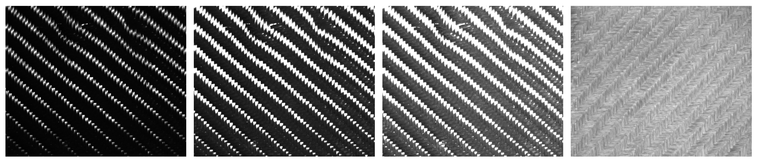
For most tests in this paper, the UD samples are positioned such that the mean fibre angle is at 90° (i.e., vertical in the images). For woven cases, half of the fibres are nominally at 90° with the remainder at 0°/180°. The sample orientation was initially set by hand, aligning the fibres with the edges of the image display in a live feed from the camera. In practice, this was rather difficult, and the ground truth orientation for all experiments has approximately 1° of uncertainty. This is the reason for the choice of relative angle measurements for the analysis (see Section 3.1) rather than the practically difficult absolute angle. It should be noted that for test samples in good imaging conditions, the difference between manually measured absolute fibre angles and that from the polarisation data fell within experimental uncertainty.

3.1. Optimal Conditions

The best results were found for the case of dark-field illumination; thus, these are analysed in detail first.

3.1.1. UD Samples

For the first test, a UD sample was placed on a computer-controlled turntable that was able to rotate the part with very high (≪1°) precision. Due to the difficulty in manually positioning the sample at a required angle, the approach was to initially align the part by trial-and-error until the polarisation method returned an average of 0° estimates across the image. The test was then to observe whether the subsequent fibre angles were correctly estimated as the table was rotated. Of course, it would have been better to test the absolute orientation of the sample by comparing the polarisation method to absolute ground truth fibre angle from the outset had the latter been more readily available. However, it is worth reiterating that estimates of the absolute angles of the fibres from polarisation data did fall within experimental error of manual measurements made with a simple protractor.

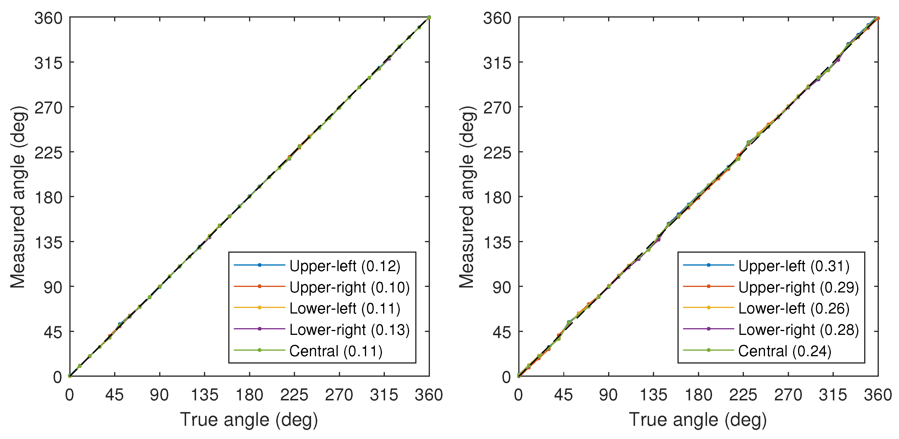
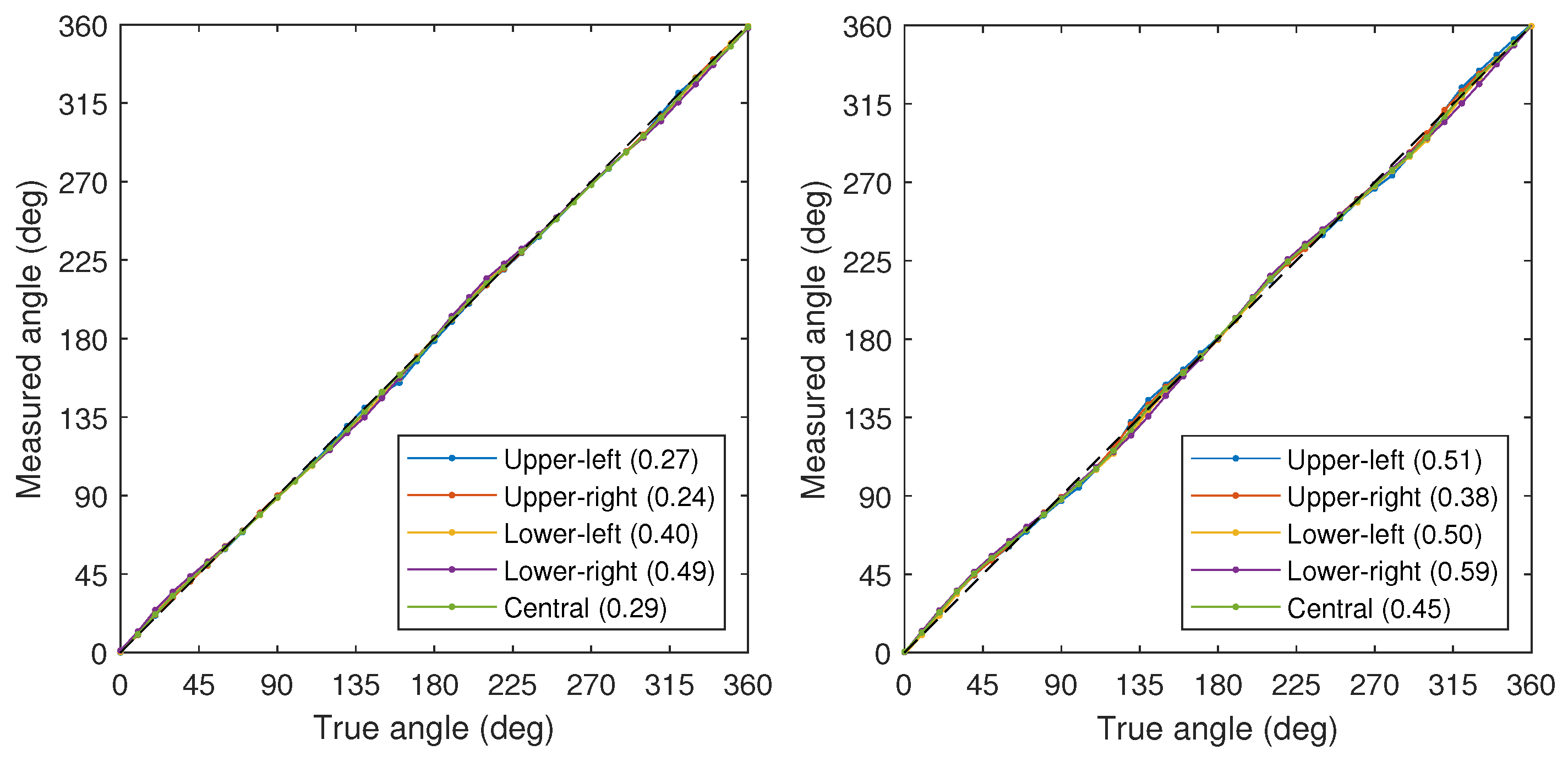
For various ROIs within the image, the estimated median angles were plotted against the turntable angle as shown in Figure 8. This shows exceptionally robust performance in the given conditions, with marginally inferior results for dry samples compared to cured ones (although this may be simply due to the greater difficulty in lining up the tows in the dry sample for data capture). Note that the turntable rotates by 360°, while outputs from the algorithm only allow angles up to 180°. For the sake of presentation, 180° has been manually added to the second half of the data points for ease of comparison.

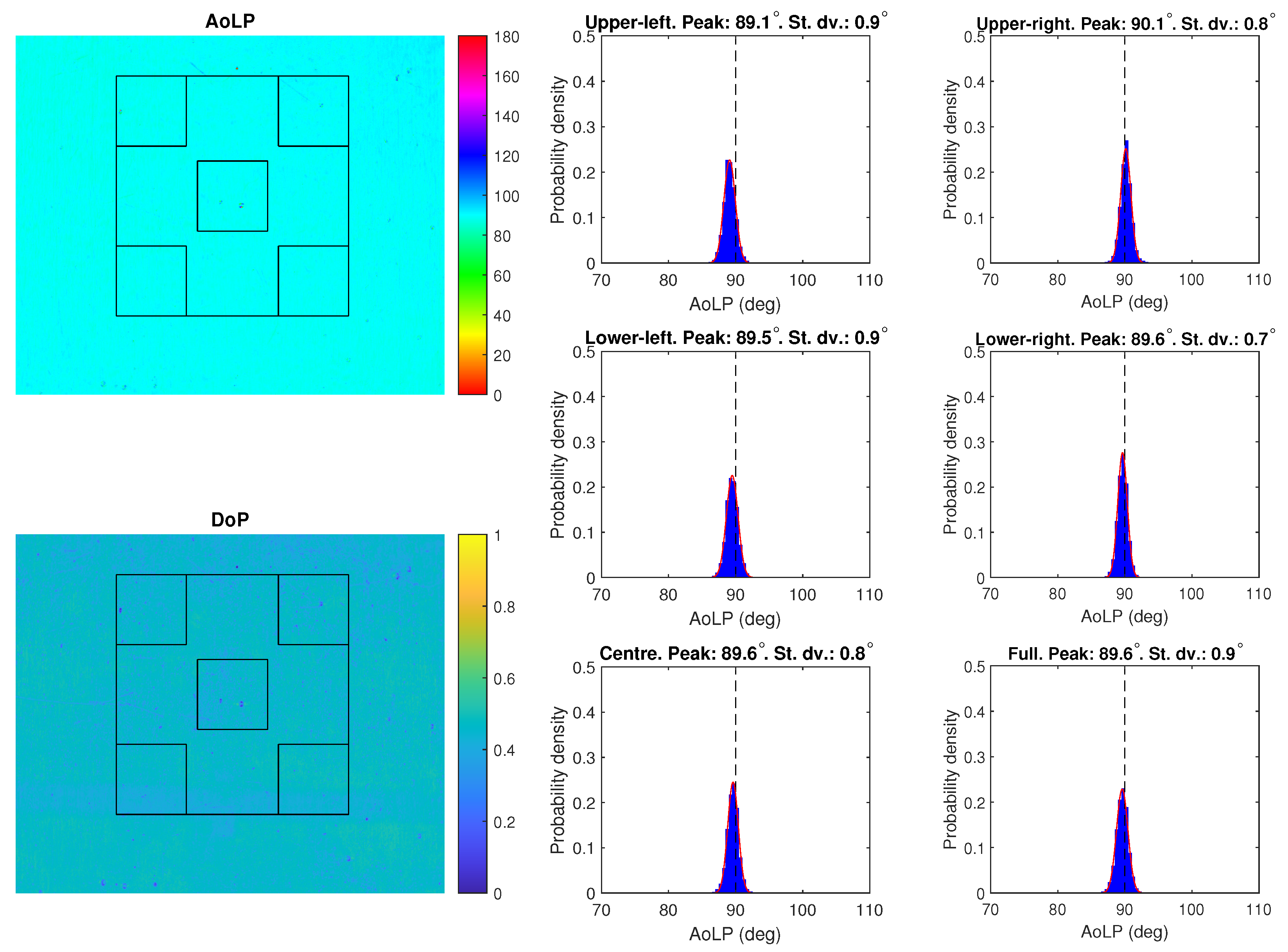
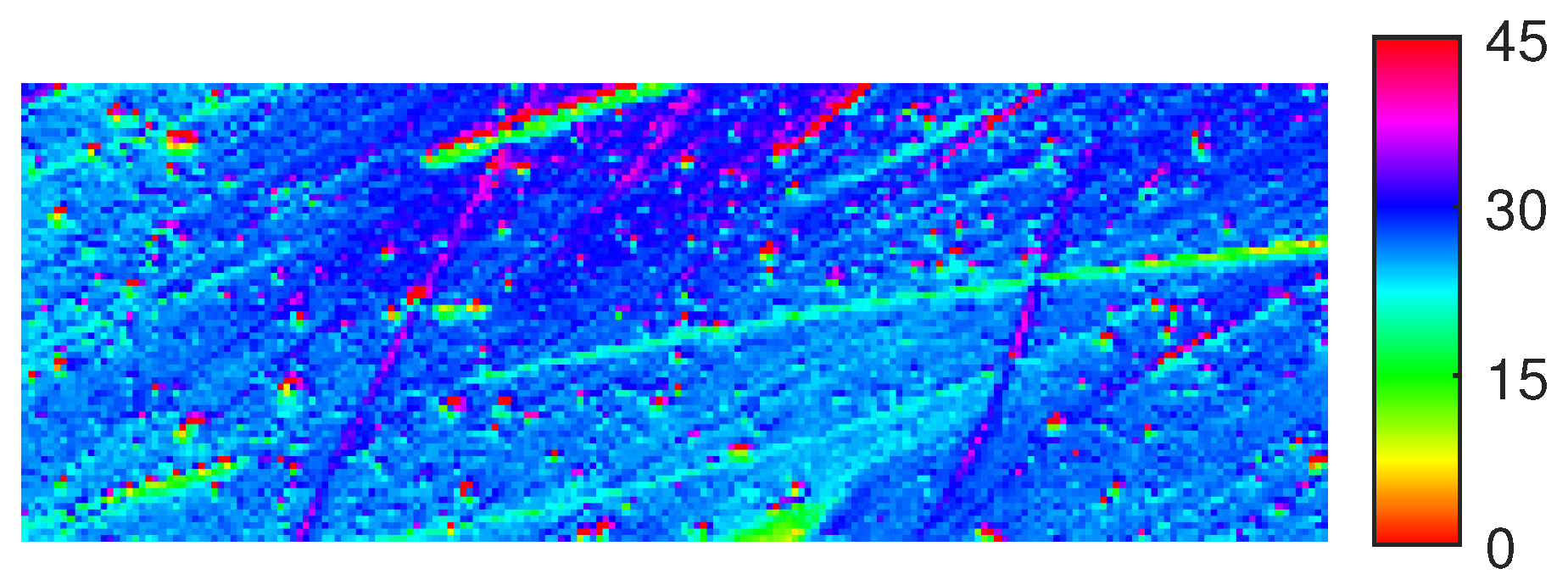
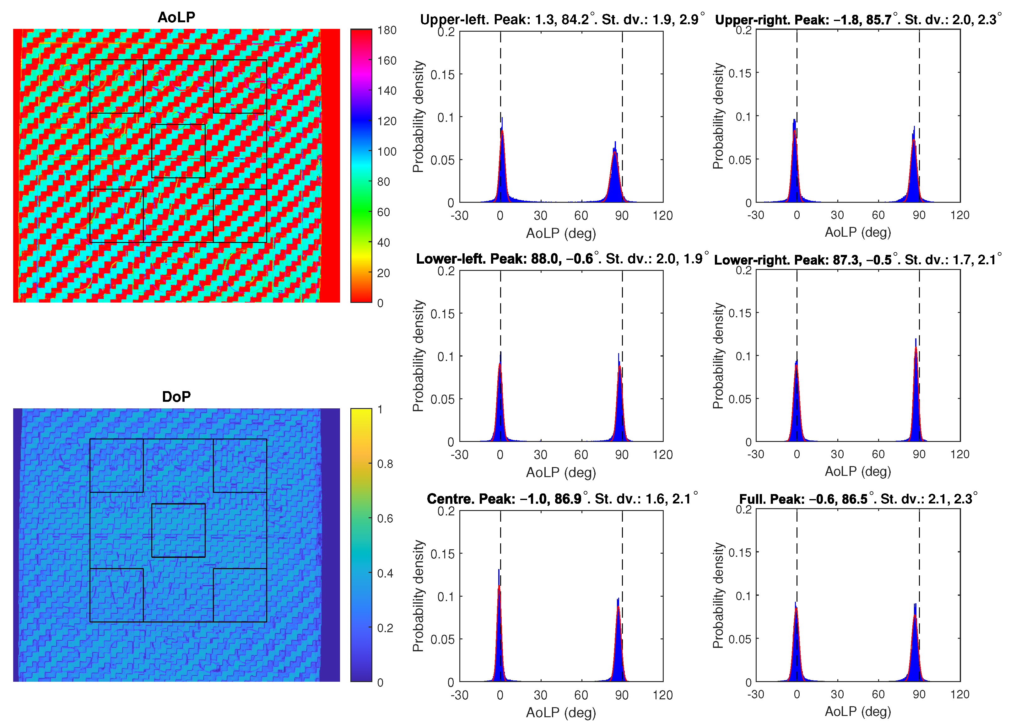
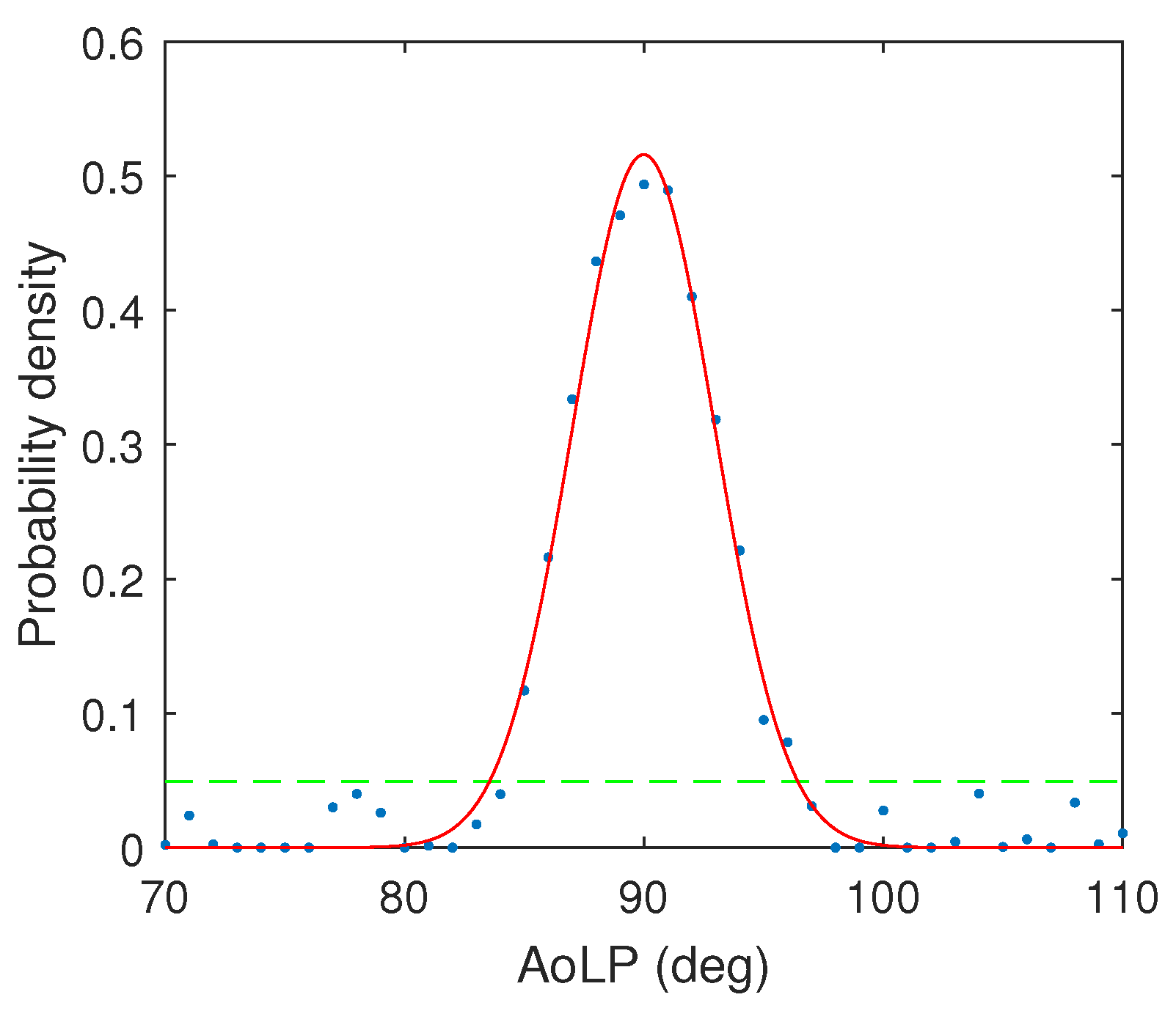
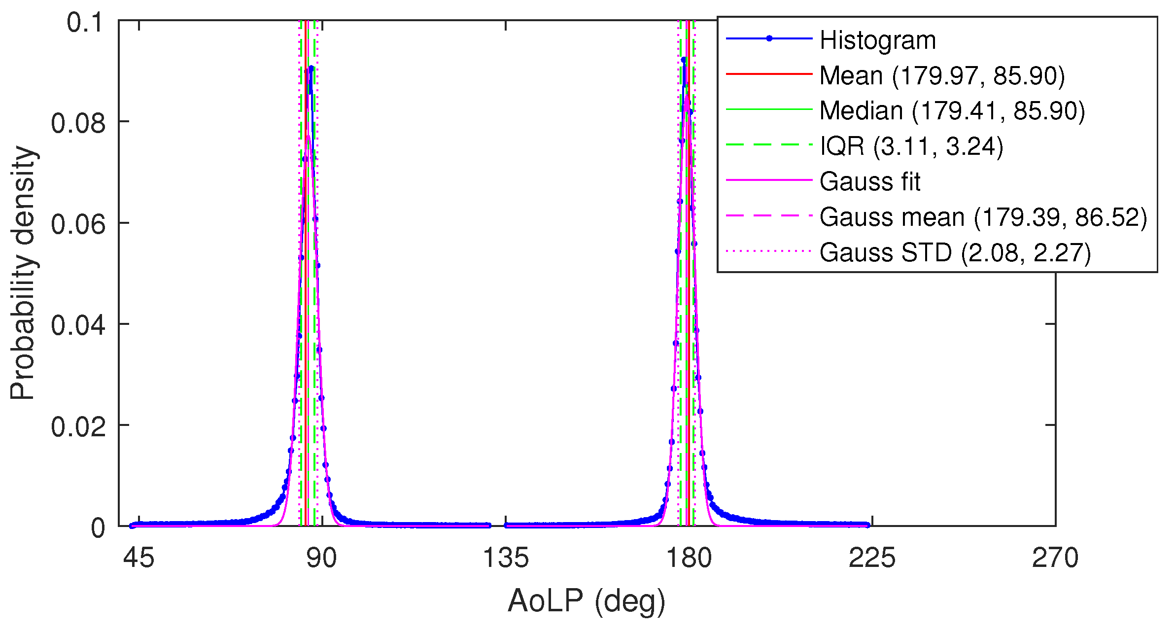
Figure 9 shows images of AoLP and DoP data for the cured sample. The AoLP image is very uniform except for a few speckles—presumably due to imperfections on the top layer and/or marks on the resin. The DoP image mostly shows high values (>0.4), meaning a correspondingly high SNR is present. Figure 9 also shows the histograms of AoLP measurements for each ROI with Gaussian curve fitting and corresponding standard deviations. Again, this demonstrates strong uniformity and values close to the expected 90°. Indeed, the results suggest that sub-degree accuracy in relative angle estimation can be attained. 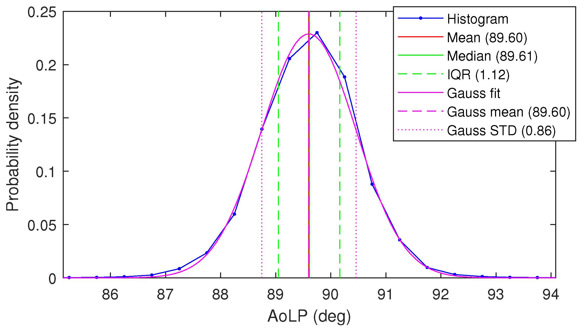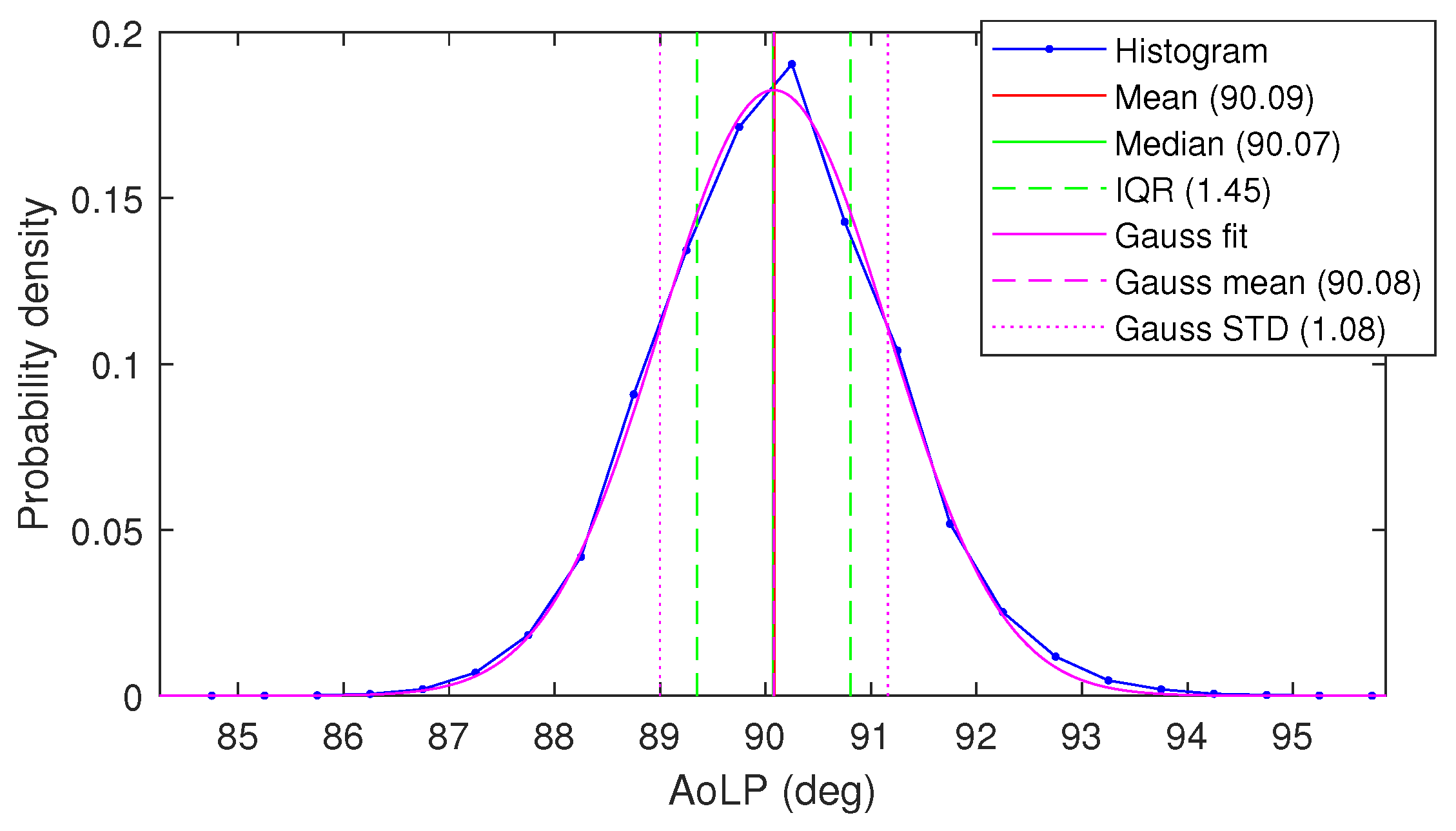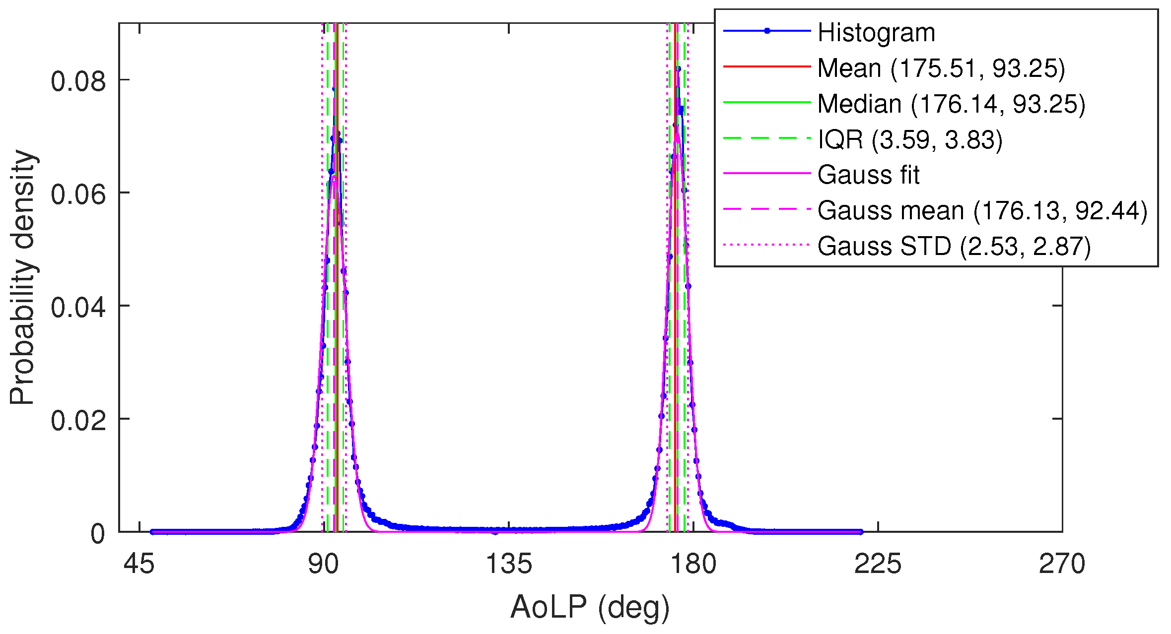Figure 10 shows a close-up of the histogram and various statistical measures used to emphasise the robustness of the AoLP to confirm the angle of orientation of carbon fibres. As observed, the difference between the mean and the median is minimal, which indicates that the likelihood of reliable estimates is high. The figure also indicates robustness of the fibre angle estimation method against the performance metric used—i.e., to show that results are not biased by the specific choice of metrics.

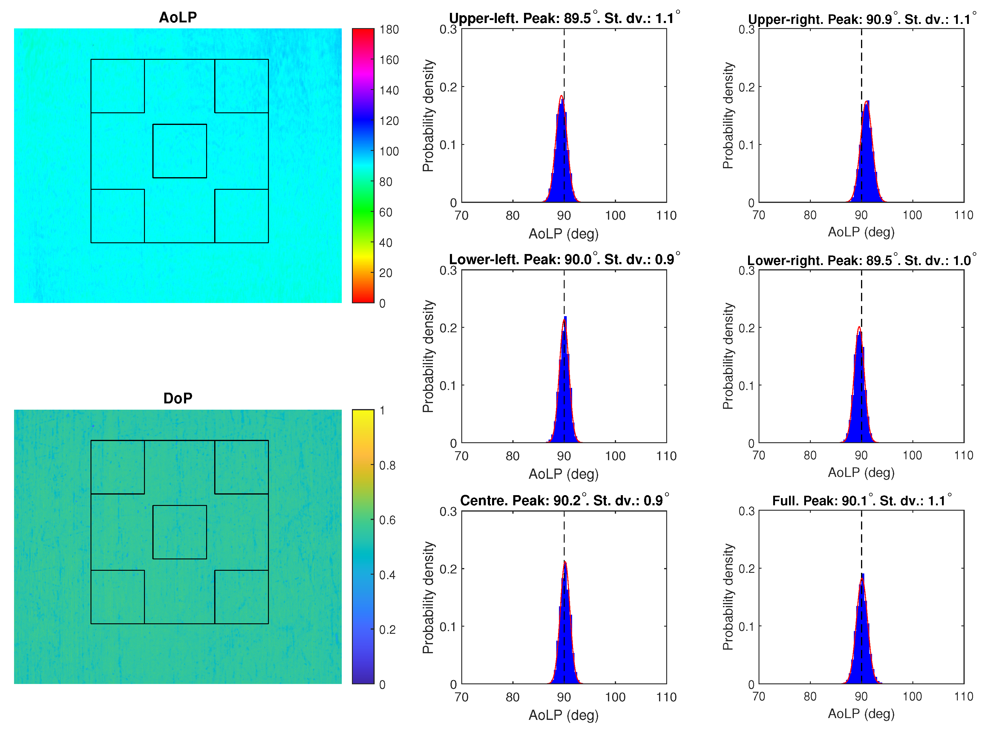
Figure 11 and Figure 12 show equivalent results for an uncured UD sample. The performance is comparable but slightly inferior with respect to the cured case in terms of the spread of data. This is presumably a consequence of both genuinely more distributed fibre angles and loose fibres reflecting light directly to the camera and would, thus, vary for different quality materials. There is also evidence of a slight shift in measured angles between different parts of the image, which will be studied further in Section 3.2.

Figure 13 shows a close-up image of a portion of dry fibre cloth (with the camera placed approximately 10 cm from the surface for this image). This shows that very fine details of the fibres can be obtained if necessary—up to single strands. However, the image also demonstrates that small particles (dust, binding agents, etc.) potentially contaminate the fibre orientation measurements. Furthermore, the AoLP values for individual fibres vary from one side of their axis to the other, as shown by the loose fibre near the top of the image at about 15°, for example. This may be a result of the three-dimensional geometry of single fibres affecting polarisation measurements, as previously observed for non-fibrous surfaces [30].

3.1.2. Non-UD Samples

Figure 14, Figure 15, Figure 16 and Figure 17 show results in optimal conditions for cured and dry woven samples. The main observation here is that both errors relative to ground truth and the standard deviations are larger. The latter is mostly explained by the presence of small but numerous transition regions between tows of fibres at each angle. A close inspection of individual tows reveals only small local variations in measurements. Data for the dry fibres clearly show the presence of waviness as, for example, in the upper-left ROI of Figure 16. Furthermore, ground truth angles are clearly not consistently 90° throughout the image. For these reasons, Figure 16 should act more as a demonstration to indicate the capabilities of the approach, rather than a test of precision.

An interim conclusion at this point is that the approach has the capability to estimate average fibre angles to a precision of at least 1° but that pixel-by-pixel estimates can be affected by a few factors such as the location of the pixel within the image (discussed below) and the transition regions between fibre directions in woven samples.

3.2. Alternative Capture Conditions

While the results above represent the best-case scenario, it is not always possible to attain such capture conditions in real-world industrial settings. This section demonstrates alternative capture conditions for comparison. The standard deviation results for various test cases are shown in

Table 3. Standard deviations (°) of measurements within the “full” ROI (see Figure 9) for various illumination conditions (23 mm lens). For the woven case, the values are simply given with the lowest number followed by the highest.

Illumination	UD Cured	UD Dry	Woven Cured	Woven Dry
Dark field	0.9	1.1	2.1, 2.3	2.5, 2.9
Bright field	1.1	1.5	4.3, 5.1	2.5, 2.7
Dome	2.1	1.3	2.3, 2.8	1.8, 1.9
Ambient	2.8	2.4	3.7, 4.3	2.4, 2.9
Point at 0°	8.8	3.0	4.3, 18.9	5.3, 11.0
Point at 45°	5.6	3.2	7.5, 15.2	3.5, 4.2
Point at 90°	3.6	4.9	4.3, 13.7	4.8, 8.2

with results from the turntable shown for the extreme case of a point source shown in Figure 18. The first observation from the table and figure is that global/large ROI measurements are still typically robust (at least with a 23 mm lens) but that pixel-level variations are often high.

As observed in Table 3, the results for bright field illumination are inferior to the dark field case for most test samples. Furthermore, the capture process was more complicated since the lights caused a specularity in the images necessitating multiple exposures to obtain the figures quoted in the table, as per the method described in Section 2.5. The dark field case by contrast, did not require this step. Indeed, the dark field and dome illuminators were the only two lighting types that did not generally require multiple exposures in order for reliable measurements to be made.

For dry samples, results from the dome light were comparable or even superior to those with dark field illumination. However, results were comparatively poor for the basic case of a cured UD sample. Upon further inspection, it was found that the reason for this is the presence of non-normal specular reflections from the resin surface to the camera, for which Fresnel Theory predicts finite polarisation even in the absence of fibres. In other words, the assumption that all polarisation is a result of the fibres breaks down.

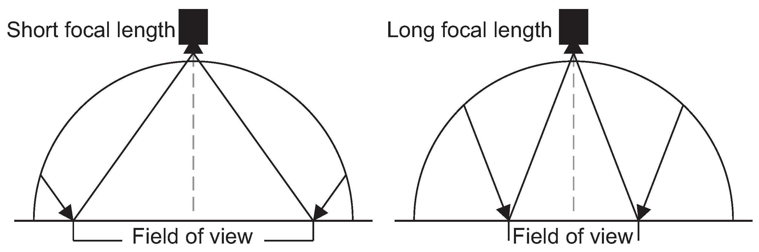
This phenomenon is best illustrated with a 12 mm lens: The representative results for which are shown in

Table 4. Standard deviations (°) of measurements within the “full” ROI (see Figure 9) for dark field and dome illumination (12 mm lens).

Illumination	UD Cured	UD Dry
Dark field	1.0	1.5
Dome	3.6	1.2

. By comparing results in this table to the corresponding cells from Table 3, the only significant difference relates to the cured UD material under the dome illuminator. This can be understood by considering that, for the shorter focal length, more of the resin surface is reflected towards the camera at a non-normal direction (strictly speaking, one should say “far-from-normal direction”), as shown in the schematic of Figure 19.

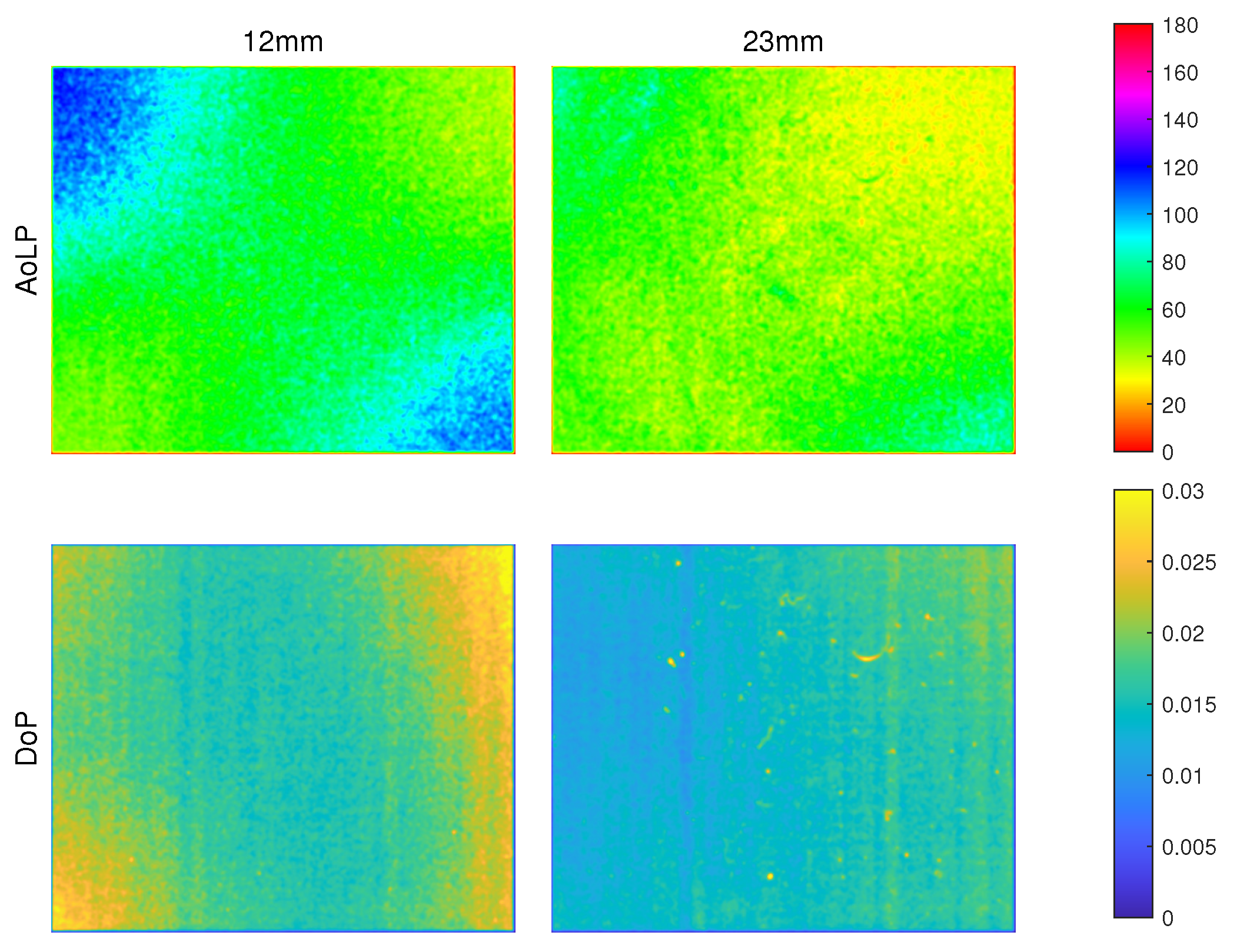
To demonstrate this effect further, Figure 20 shows AoLP and DoP images for a pure cured resin surface (i.e., the planar resin matrix with no fibres embedded). In this case, there are no anisotropic conducting fibres to polarise light, meaning that any observed pattern is due to specular reflection following phenomena studied elsewhere in the literature [5,22]. This is apparent from the fact that the four corners of the image follow an obvious pattern, but that the effect is less noticeable for the longer focal length, where less non-normal specular reflectances are present.

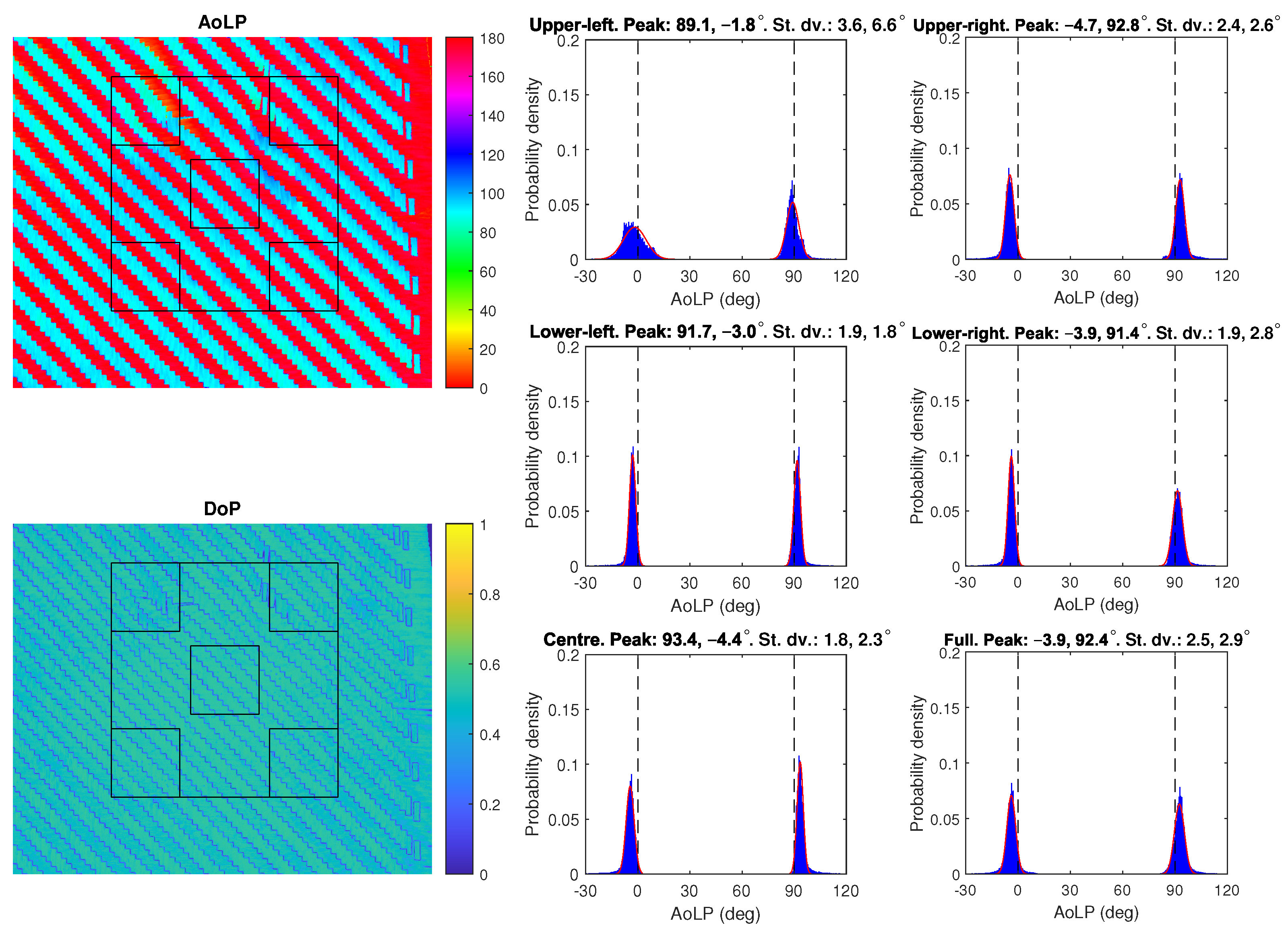
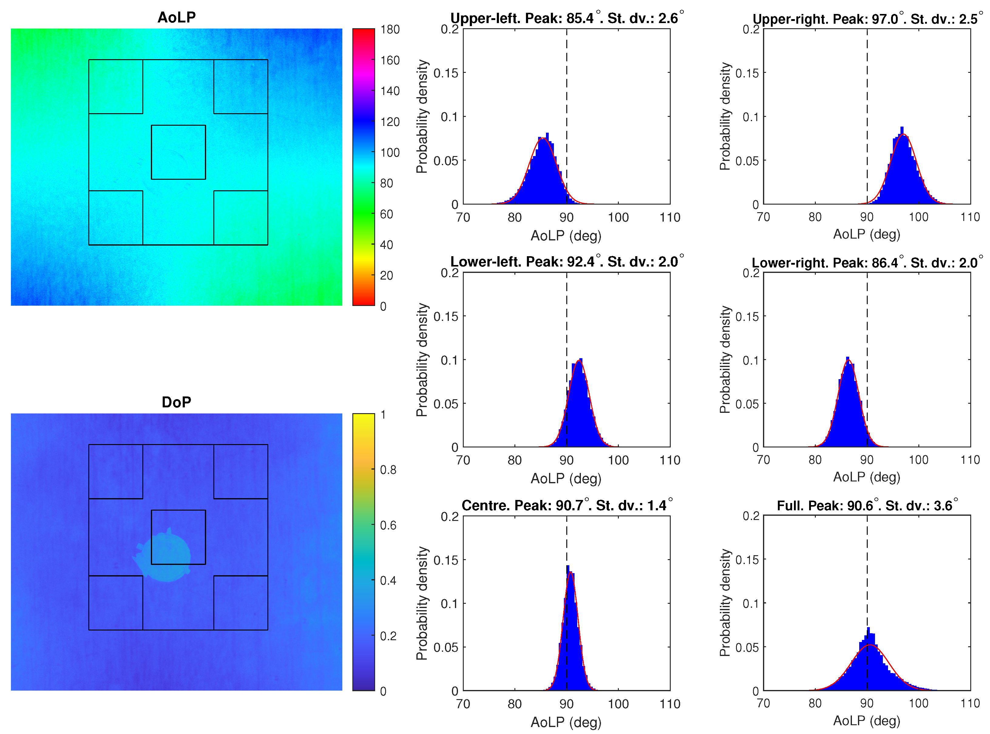
Figure 21 shows results for the cured UD sample with a 12 mm lens under the dome. The AoLP image demonstrates that the phenomenon in Figure 20, unfortunately, carries over into an image with carbon fibre in the resin. The histogram peaks for the central and full ROIs show good estimates of the true fibre angles, but the outer ROIs show huge (>5°) deviations as a result of the specular reflections from the resin. 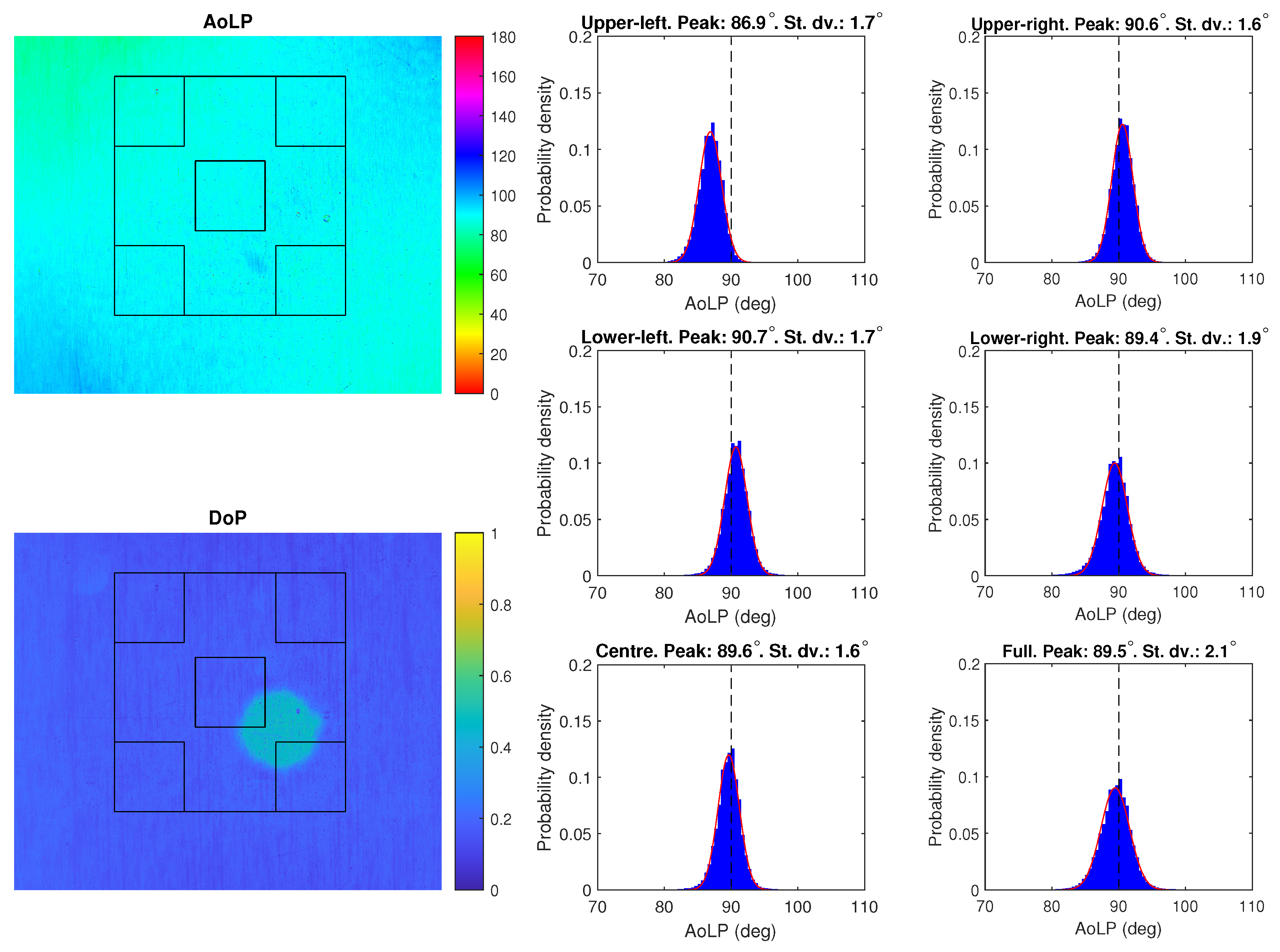While this effect is particularly extreme here (the experiment for obtaining Figure 21 was specifically devised to exaggerate the effect), it is still apparent to a lesser-degree when using a 23 mm lens, as in Figure 22. It can also be observed to a small extent in some of the earlier results, such as in Figure 11.

The fourth row of Table 3 shows the measured standard deviations under ambient illumination—in this case, light from overhead fluorescent strip lights in a small laboratory and a multitude of consequent reflections around the room. Not surprisingly, the results are inferior to the optimal case. Furthermore, other forms of ambient light would presumably generate different results. However, this test does demonstrate scope for some measurements to be taken without specialised illumination in certain environments depending on the variability of conditions and the required precision.

The final results from Table 3 show standard deviations with the surface illuminated by a single LED. These tests are included to help understand the optical properties of the materials, rather than as realistic scenarios for industrial environments. The results for the point sources are generally poor—especially for cured samples with a parallel reflectance plane (a less dramatic reverse of this trend is true for dry samples for reasons not yet fully understood). In the table, the standard deviations for woven materials are simply listed in numerical order; although upon close examination, it was found that the direction corresponding to the higher values followed a similar trend to the UD samples. While this wide distribution of measured angles limits the applicability of data at the pixel level, the average angle measurements over wider ROIs proved more useful, as shown by results of a cured UD sample on the turntable, for example (Figure 18).

3.3. Non-Planar Surfaces

So far, this paper has considered planar components that are parallel to the image plane. The first experiment for investigating more general components aimed to image the planar UD cured sample under dark field illumination but with the surface inclined at an angle of 15° to the image plane. This was performed twice: The first was performed such that the fibres themselves were inclined relative to the image plane, and the second was performed such that each fibre was parallel to the image plane with neighbouring fibres moving progressively further from the camera. The purpose of this test was to assess the importance of any angular offset between the image plane and the sample part. The results were very promising, with numerical differences to the non-inclined plane that were insufficiently large to establish any real difference (full experimental data are available in Data Availability Statement).

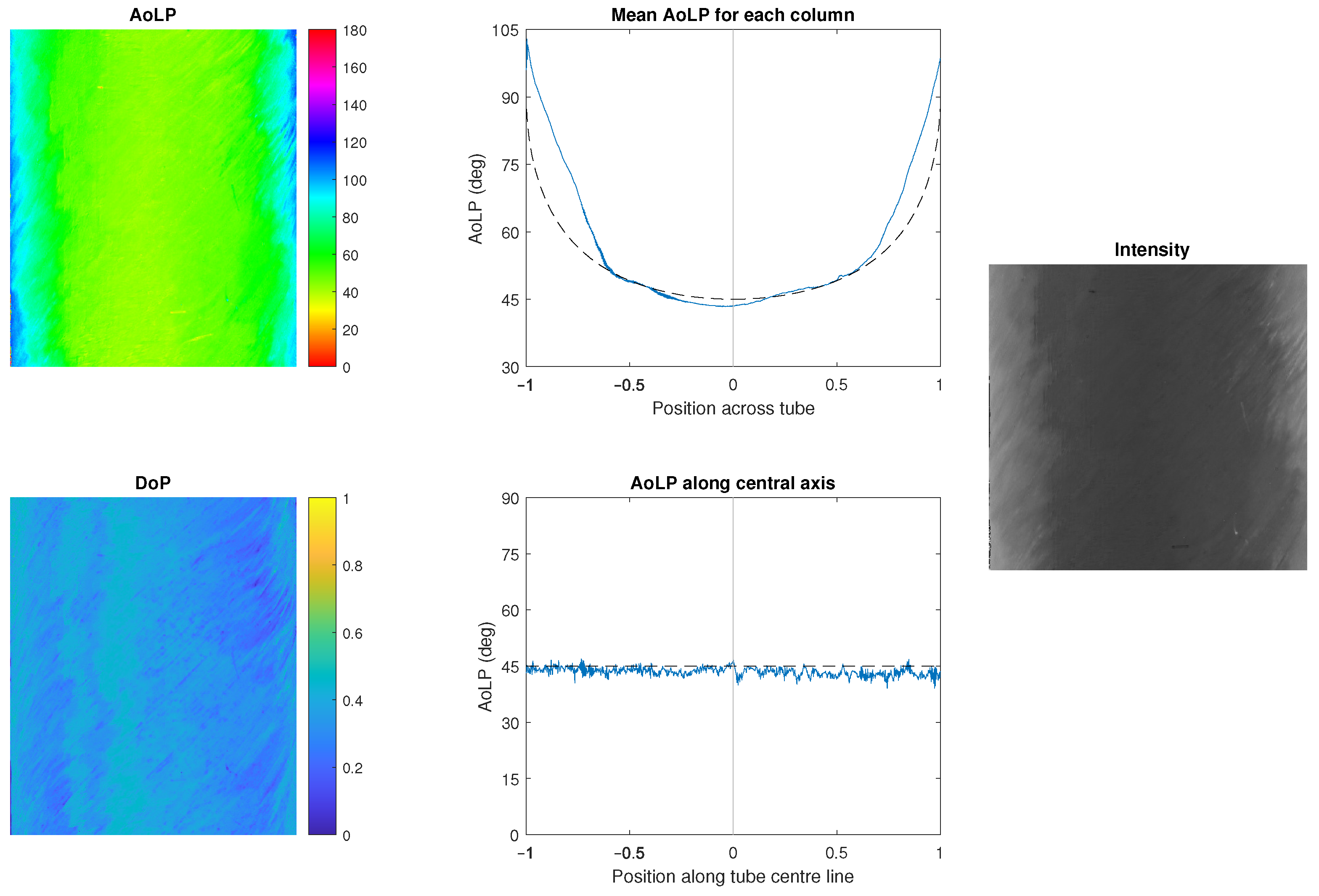
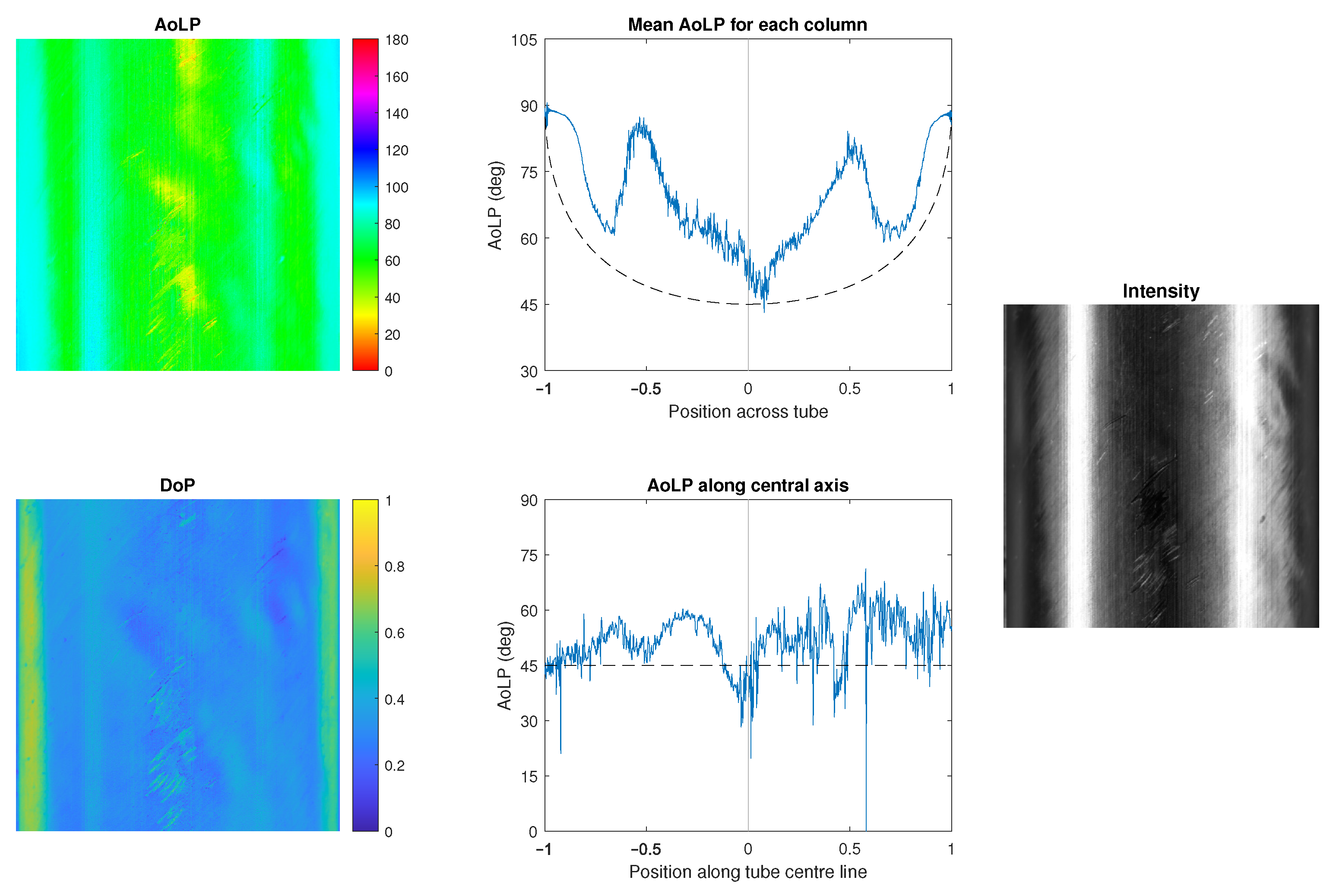
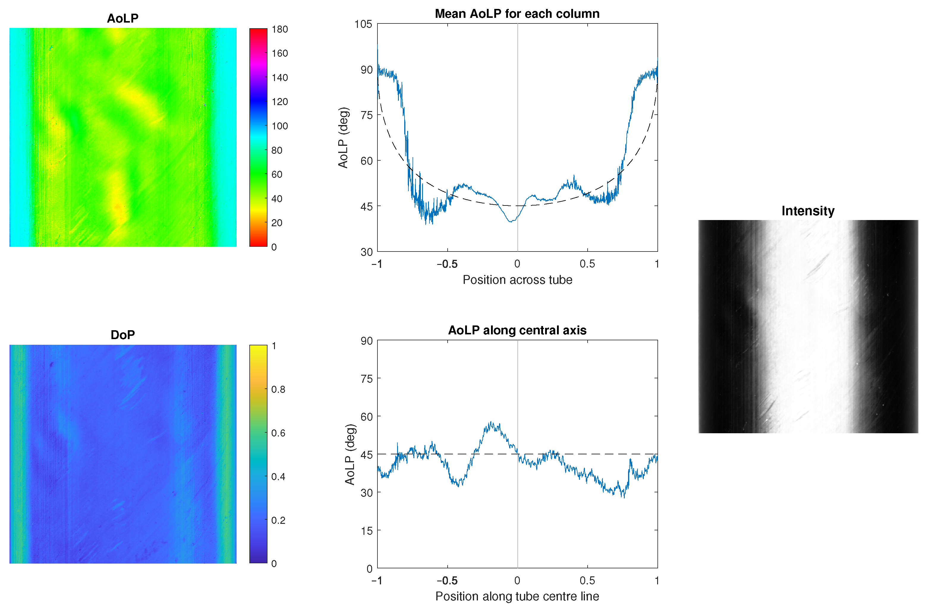
Unfortunately, the results for non-planar surfaces mostly demonstrated poor accuracy. However, they are briefly presented here as discoveries have been made that may prove useful for future research. Figure 23 shows polarisation data for a section of a cured UD tube under dark field illumination. The tube is constructed in a manner such that the angle between the fibres and the axis of the tube is 45°. The DoP image shows a nonuniform pattern with especially high values near the occluding contours. This is most likely due to specular and/or diffuse reflection obeying the Fresnel theory [5,22] in combination with the tendency of AoLP to align with the fibres. As a result, specular reflections from the light sources caused erroneous angle measurements where this occurred. The graphs in Figure 23 further demonstrate these complications, with specularities at positions of approximately −0.5 and +0.5 across the tube.

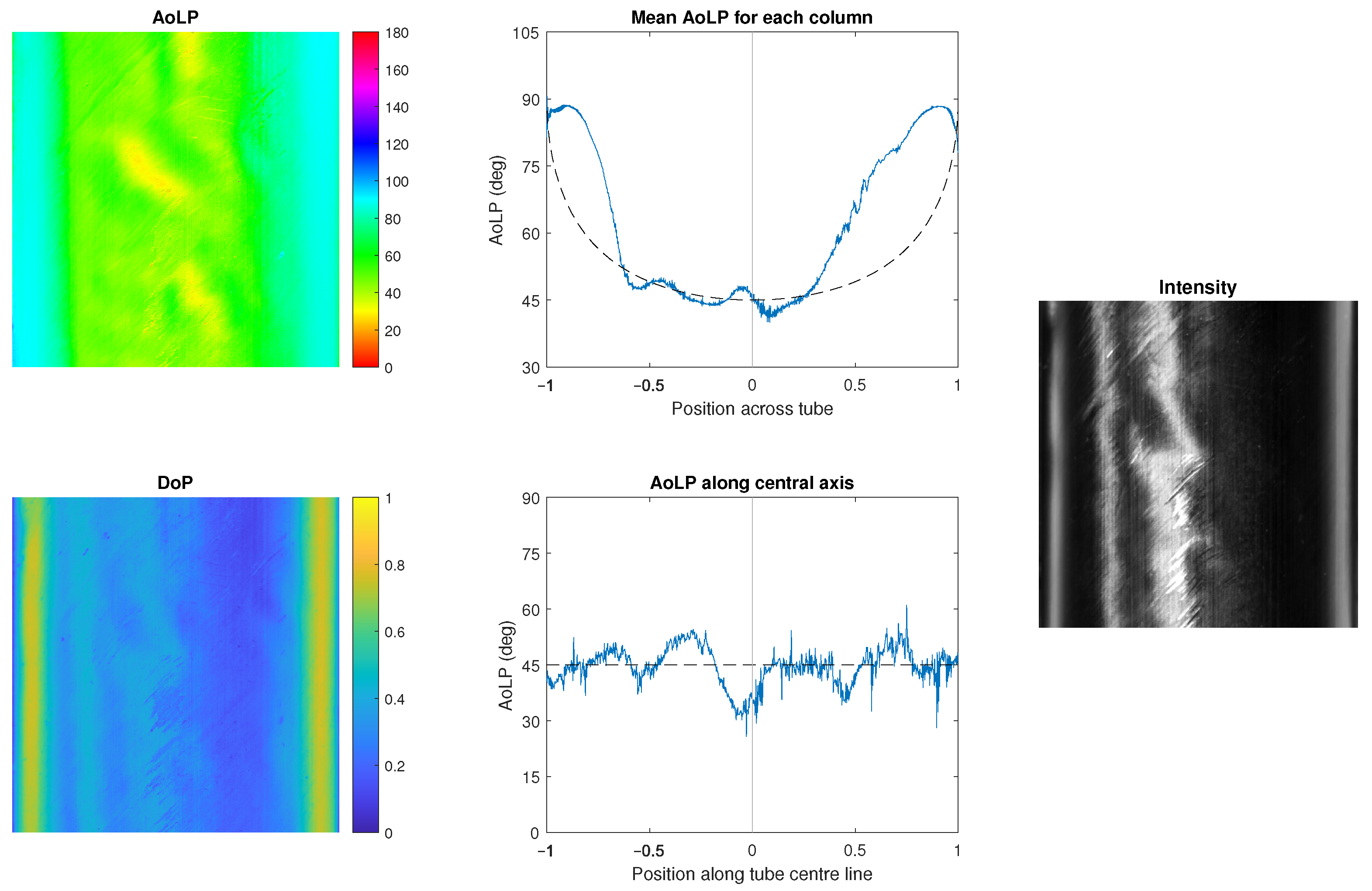
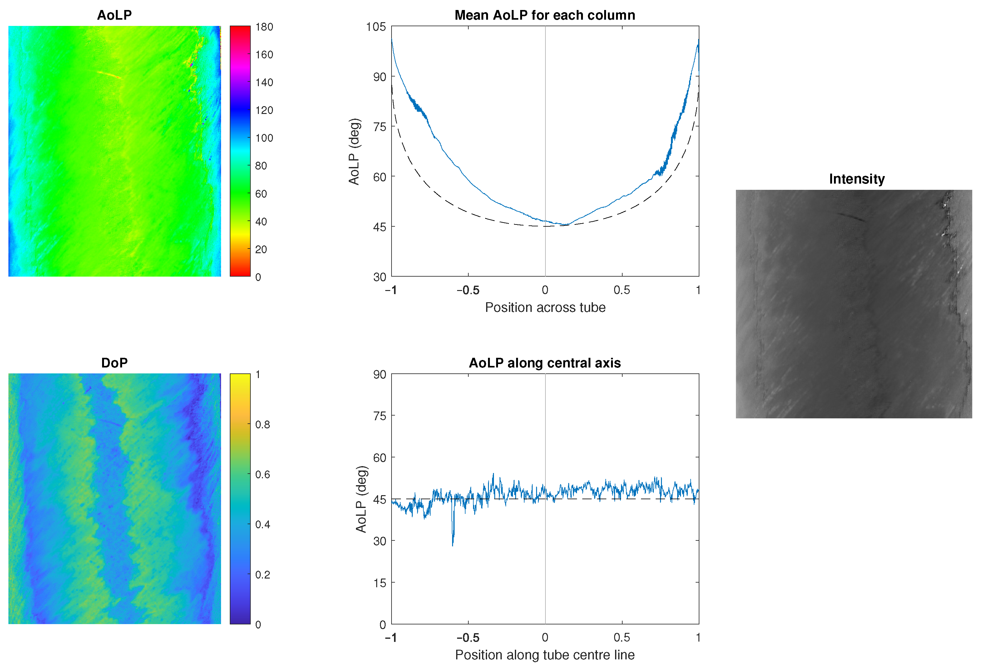
In an effort to minimise the complications above, the data for the tube were recaptured by using ambient and dome illumination, as shown in Figure 24 and Figure 25, respectively. The motivation for this was that the complications with dark field illumination might be reduced with more uniform lighting. It should be noted that the component was not completely inside the dome for Figure 24 for practical reasons, meaning that the lighting was not truly hemispherical, with only minimal illumination emerging from grazing angles. The results are indeed superior but still inadequate for most real industrial applications.

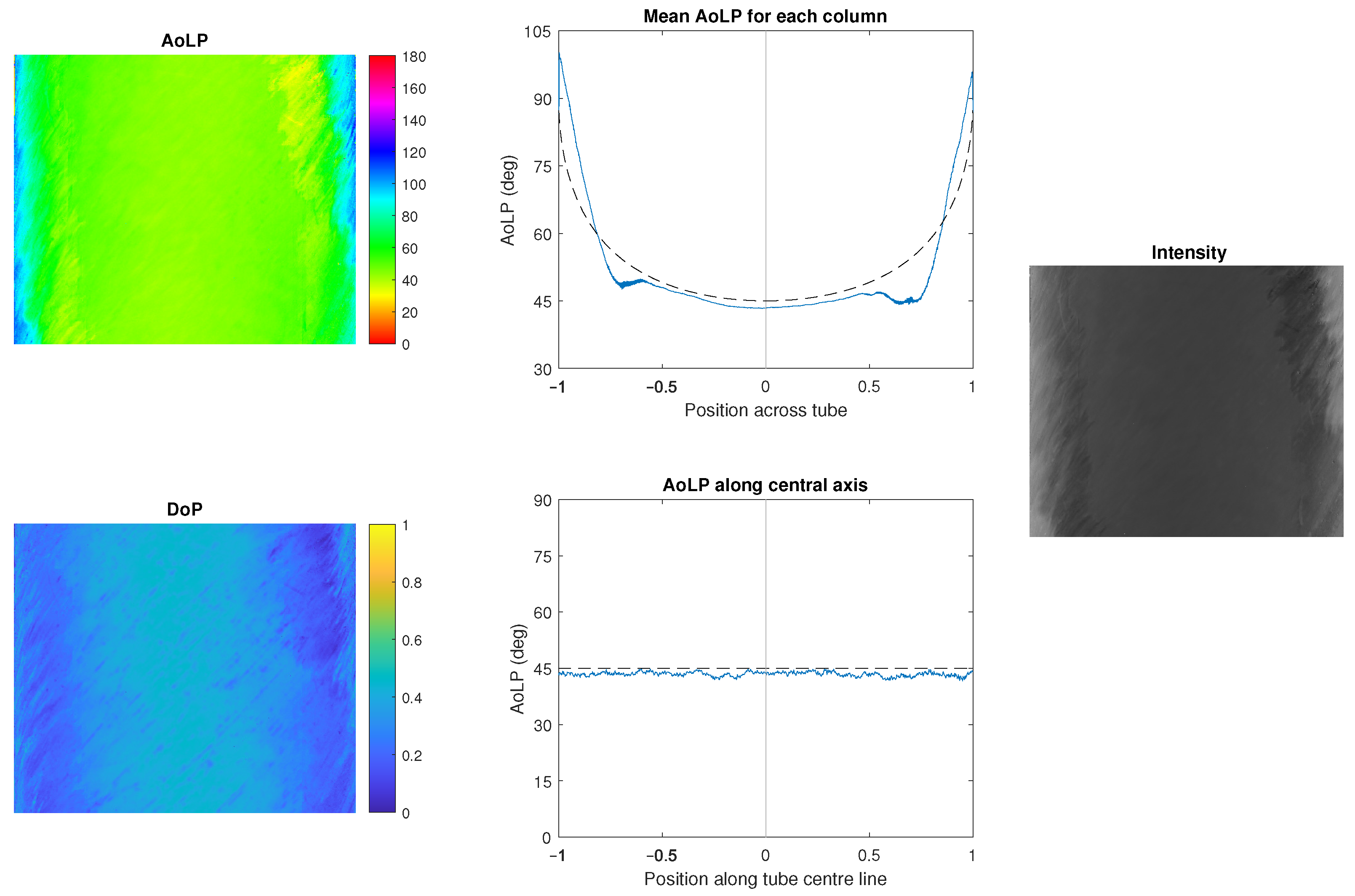
Figure 26, Figure 27 and Figure 28 show the results for a similar tube but with UD dry material wrapped around. Here, we see much more predictable results since the complications of non-normal specular reflections from the resin are no longer present. The bumps on the dome illuminator image are thought to be due to the fact that the component did not fit fully inside.

In summary, the results for the tube correctly showed AoLP approaching 90° at the occluding contours (see Data Availability Statement for details of theoretical prediction) and 45° in the centre of the tube. However, competition between the effects described by the Fresnel theory for specularities and the alignment of the electric field of the reflected light with the fibres means that many parts of the images follow a very complicated (and difficult to model) pattern. This is further complicated by the difficulty in manufacturing the tube to a high degree of precision, as can be seen in some parts of the AoLP in Figure 24 that have lower-than-expected values, for example.

4. Discussion

The results presented in the previous section are highly varied in terms of accuracy and applicability. At best, they demonstrate highly repeatable sub-degree measurements of fibre angles in dark field illumination. At worst, non-planar components proved difficult to inspect—although the nature of the inaccuracies were, at least, well understood in a phenomenological sense.

For the best-case results, it is easy to imagine an inspection system based on the proposed method that is integrated into a manufacturing line. This could take many forms. For instance, it could be used for small scale inspection of a high-precision component that is either planar or possesses a large radius of curvature. Alternatively, for some lower-precision/resolution applications, the method may be beneficial with a large working distance. However, installation and control of dark field illumination may be impractical in such a case.

A different approach might be to employ an integrated system, whereby the dark field lights and the camera are all attached to an end effector of a robot arm or gantry system that traverses the surface, scanning the part sequentially. This would maximise the uniformity of illumination throughout the capture. Indeed, it may prove beneficial to switch the technology to a line-scanning approach for some applications should such a version of the polarisation sensor ever be commercialised. An area-scan surface-traversal approach has already been proven by applying non-polarisation machine vision technology by Profactor [39]. If a three-dimensional CAD model of the part is available (typically the case), then a three-dimensional part can be inspected provided that the curvature is sufficiently low as to prevent complications such as those described in Section 3.3. The inclined-plane experiments in Section 3.3 support this possibility, showing that a small misalignment between the image plane and surface patch has negligible implications on precision. In any case, given the inferior results of ambient illumination compared to that of dark field in Table 3, the dark field lights should be sufficiently bright as to drown out ambient light as much as possible. In fact, a few experiments were conducted as part of this research study involving the capture of two images in rapid succession: one with dark field and ambient light and one with only ambient light. The latter image was then subtracted from the former, effectively only leaving the dark field component. However, the improvement in results was too small/negligible to be reported in this paper.

Dome illumination might be an effective option for situations that are both practical for such an illuminator to be present on the production line/inspection system and where ambient illumination is unpredictable. The results in this paper suggest superior results for woven materials using the dome illuminator, although this is minor and inconclusive. Under ambient illumination, the results are less predictable, as one might have expected. However, they do demonstrate potential application for lower-precision applications. Indeed, this might be regarded as a strength of the method because inspection using uncontrolled illumination is a highly desirable but is a seldom attained goal—even at low-precision.

While the results for the tube were of low quality, there is some hope for the inspection of parts during a draping process for some applications based on the promising output for dry fibres wrapped around the tube under dome and ambient illumination (Figure 27 and Figure 28).

One weakness of the paper is the difficulty in obtaining reliable ground truth absolute angle values for comparison to the experiment. Regardless of this, the relative values are all well within 1° precision for planar surfaces, provided that there is some initial reference to which other results can be measured against. Finally, it should be noted that, in most cases, individual pixel measurements are of limited use due to relatively high (typically >1°) standard deviations in values. Instead, global measurements or average values over small regions should be used as outputs from the method.

In relation to alternative technologies for composite part inspection, the methods in this paper are largely complementary. The approach is financially and computationally much cheaper than most others and relatively straightforward to incorporate into manufacturing lines. The method is also fast and requires little installation time or infrastructure. On the other hand, polarisation methods do require careful consideration of illumination—especially for high-precision applications—and are only able to inspect top layers. That said, such a system could potentially be embedded onto a production line such that each layer is inspected in situ during the layup process. Another weakness of polarisation is that the method is only sensitive to defects/misalignments that occur within the plane of the surface. While this precludes the detection of certain problems, it is believed that the majority of defects do at least partially manifest within the plane and so are theoretically detectable using polarisation information.

5. Conclusions

This paper has demonstrated the capabilities and limitations of polarisation imaging technology as applied to CFRP component inspections. In the best cases, the average relative angles over specific regions of interest were measured to less than one quarter of a degree, with standard deviations less than one degree. Other situations, however, had much higher standard deviations, often over 2°, as shown in Table 3. Cases have been identified where the approach can be embedded into an existing production line (e.g., close-up inspection of UD and woven materials under dome illumination or mid-range measurements of UD components under dark-field illumination). Cases have also been identified where the outputs are of poor quality such as for highly curved surfaces or short focal lengths where specularities are present on resin. In summary, the paper has shown great promise for the technology but also that there are many potential complications present, meaning that the design features of an inspection system may vary depending on the application in question.

The aim of future work will be to more closely inspect the small differences in precision for woven materials compared to UD and to parametrise the limits of curvature for which robust measurements can be made—or even design illumination to permit full-scale inspection of three-dimensional parts. We also hope to further study the effects of specular reflection to introduce corrective factors for short focal lengths (i.e., to address the weaknesses identified in Figure 21). As mentioned in the introduction, the method theoretically allows a more general inspection process to localise defects in CFRP samples; thus, a natural follow-on study would verify this. Finally, the methods should be trialed in real-world manufacturing and inspection settings such as in a layup laboratory or above a ply cutter.

References

1. Das, T.K.; Ghosh, P.; Das, N.C. Preparation, development, outcomes, and application versatility of carbon fiber-based polymer composites: A review. Adv. Compos. Hybrid Mater. 2019, 2, 214–233. [Google Scholar] [CrossRef]
2. Yokozeki, T.; Ogasawara, T.; Ishikawa, T. Effects of fiber nonlinear properties on the compressive strength prediction of unidirectional carbon–fiber composites. Compos. Sci. Technol. 2005, 65, 2140–2147. [Google Scholar] [CrossRef]
3. Vallons, K.; Duque, I.; Lomov, S.; Verpoest, I. Fibre orientation effects on the tensile properties of biaxial carbon/epoxy NCF composites. In Proceedings of the ICCM International Conference on Composite Materials, Edinburgh, UK, 27–31 July 2009. [Google Scholar]
4. Rudberg, T.; Nielson, J.; Henscheid, M.; Cemenska, J. Improving AFP Cell Performance. SAE Int. J. Aerosp. 2014, 7, 317–321. [Google Scholar] [CrossRef]
5. Atkinson, G.A.; Ernst, J.D. High-sensitivity analysis of polarization by surface reflection. Mach. Vis. Appl. 2018, 29, 1171–1189. [Google Scholar] [CrossRef] [Green Version]
6. Djordjevic, B.; Suite, C.; Burnie, G. Nondestructive test technology for the composites. In Proceedings of the International Conference of the Slovenian Society for Non-Destructive Testing, Ljubljana, Sloveni, 1–3 September 2009; pp. 259–265. [Google Scholar]
7. Vaara, P.; Leinonen, J. Technology Survey on NDT of Carbon-Fiber Composites; Technical Report; Kemi-Tornio University of Applied Sciences: Kemi, Finland, 2012. [Google Scholar]
8. Nelson, R.J.; Smith, R.A.; Mienczakowski, M. Ply-orientation measurements in composites using structure-tensor analysis of volumetric ultrasonic data. Compos. Part A Appl. Sci. Manuf. 2018, 104, 108–119. [Google Scholar] [CrossRef] [Green Version]
9. Weissenböck, J.; Amirkhanov, A.; Li, W.; Reh, A.; Amirkhanov, A.; Gröller, E.; Kastner, J.; Heinzl, C. FiberScout: An Interactive Tool for Exploring and Analyzing Fiber Reinforced Polymers. In Proceedings of the IEEE Pacific Visualization Symposium, Yokohama, Japan, 4–7 March 2014; pp. 153–160. [Google Scholar] [CrossRef]
10. Wirjadi, O.; Schladitz, K.; Easwaran, P.; Ohser, J. Estimating fibre direction distributions of reinforced composites from tomographic images. Image Anal. Stereol. 2016, 35, 167–179. [Google Scholar] [CrossRef] [Green Version]
11. Teßmann, M.; Mohr, S.; Gayetskyy, S.; Haßler, U.; Hanke, R.; Greiner, G. Automatic determination of fiber-length distribution in composite material using 3D CT data. EURASIP J. Adv. Signal Process. 2010, 2010, 545030. [Google Scholar] [CrossRef] [Green Version]
12. Garcea, S.; Wang, Y.; Withers, P. X-ray computed tomography of polymer composites. Compos. Sci. Technol. 2018, 156, 305–319. [Google Scholar] [CrossRef]
13. Shi, L.; Wu, S. Automatic Fiber Orientation Detection for Sewed Carbon Fibers. Tsinghua Sci. Technol. 2007, 12, 447–452. [Google Scholar] [CrossRef]
14. Şerban, A. Automatic detection of fiber orientation on CF/PPS composite materials with 5-harness satin weave. Fibers Polym. 2016, 17, 1925–1933. [Google Scholar] [CrossRef]
15. Zambal, S.; Palfinger, W.; Stöger, M.; Eitzinger, C. Accurate fibre orientation measurement for carbon fibre surfaces. Pattern Recognit. 2015, 48, 3324–3332. [Google Scholar] [CrossRef]
16. Schöberl, M.; Kasnakli, K.; Nowak, A. Measuring Strand Orientation in Carbon Fiber Reinforced Plastics (CFRP) with Polarization. In Proceedings of the World Conference on Non-Destructive Testing, Munich, Germany, 13–17 June 2016. [Google Scholar]
17. Carroll, J. Researchers Deploy Polarization Camera for Carbon Fiber Inspection. 2018. Available online: https://www.vision-systems.com/print/content/16752033 (accessed on 21 June 2021).
18. Atkinson, G.A.; Thornton, T.J.; Peynado, D.I.C.; Ernst, J.D. High-precision polarization measurements and analysis for machine vision applications. In Proceedings of the European Workshop on Visual Information Processing, Tampere, Finland, 26–28 November 2018. [Google Scholar]
19. Wolff, L.B.; Boult, T.E. Constraining Object Features Using a Polarisation Reflectance Model. IEEE Trans. Patt. Anal. Mach. Intell. 1991, 13, 635–657. [Google Scholar] [CrossRef]
20. Wolff, L.B. Diffuse-reflectance Model for Smooth Dielectric Surfaces. J. Opt. Soc. Am. A 1994, 11, 2956–2968. [Google Scholar] [CrossRef]
21. Wolff, L.B. Polarization Vision: A New Sensory Approach to Image Understanding. Image Vis. Comp. 1997, 15, 81–93. [Google Scholar] [CrossRef]
22. Atkinson, G.A.; Hancock, E.R. Recovery of Surface Orientation from Diffuse Polarization. IEEE Trans. Image Proc. 2006, 15, 1653–1664. [Google Scholar] [CrossRef] [PubMed] [Green Version]
23. Wolff, L.B.; Mancini, T.A.; Pouliquen, P.; Andreou, A. Liquid crystal polarization camera. IEEE Trans. Robot. Autom. 1997, 13, 195–203. [Google Scholar] [CrossRef]
24. Miyazaki, D.; Takashima, N.; Yoshida, A.; Harashima, E.; Ikeuchi, K. Polarization-based Shape Estimation of Transparent Objects by Using Raytracing and PLZT Camera. Proc. SPIE 2005, 5888, 588801. [Google Scholar]
25. Wolff, L.B. Polarization camera for computer vision with a beam splitter. J. Opt. Soc. Am. A 1994, 11, 2935–2945. [Google Scholar] [CrossRef]
26. Pezzaniti, J.L.; Chenault, D.; Roche, M.; Reinhardt, J.; Pezzaniti, J.P.; Schultz, H. Four camera complete Stokes imaging polarimeter. In SPIE Polarization: Measurement, Analysis, and Remote Sensing, Proceedings of the SPIE Defense and Security Symposium, Orlando, FL, USA, 16–20 March 2008; SPIE: Bellingham, WA, USA, 2008; Volume 6972. [Google Scholar]
27. 4D Technology. Available online: https://www.4dtechnology.com/products/polarimeters/polarcam (accessed on 11 April 2019).
28. The Ricoh Company Ltd. Polarisation Camera. Available online: https://www.ricoh.com/technology/tech/051_polarization.html (accessed on 25 June 2021).
29. Sony XCG-CP510. Available online: https://www.image-sensing-solutions.eu/XCG-CP510.html (accessed on 11 April 2019).
30. Atkinson, G.A.; Hancock, E.R. Shape Estimation using Polarization and Shading from Two Views. IEEE Trans. Pattern Anal. Mach. Intell. 2007, 29, 2001–2017. [Google Scholar] [CrossRef]
31. Atkinson, G.A. Polarisation Photometric Stereo. Comp. Vis. Image Underst. 2017, 160, 158–167. [Google Scholar] [CrossRef] [Green Version]
32. York, T.; Powell, S.B.; Gao, G.S.; Kahan, L.; Charanya, T.; Saha, D.; Roberts, N.W.; Cronin, T.; Marshall, J.; Achilefu, S.; et al. Bioinspired Polarization Imaging Sensors: From Circuits and Optics to Signal Processing Algorithms and Biomedical Applications. Proc. IEEE 2014, 102, 1450–1469. [Google Scholar] [CrossRef] [PubMed]
33. Schechner, Y.Y.; Narashimhan, S.G.; Nayar, S.K. Polarization-based Vision through Haze. Appl. Opt. 2003, 42, 511–525. [Google Scholar] [CrossRef] [PubMed]
34. Powell, S.B.; Garnett, R.; Marshall, J.; Rizk, C.; Gruev, V. Bioinspired polarization vision enables underwater geolocalization. Sci. Adv. 2018, 4, eaao6841. [Google Scholar] [CrossRef] [PubMed] [Green Version]
35. Koshikawa, K.; Utsu, M.S.T.; Takemura, K. Polarized Near-Infrared Light Emission for Eye Gaze Estimation. In Proceedings of the ACM Symposium on Eye Tracking Research and Applications, Stuttgart, Germany, 2–5 June 2020. [Google Scholar] [CrossRef]
36. Hecht, E. Optics, 3rd ed.; Addison Wesley Longman: Menlo Park, CA, USA, 1998. [Google Scholar]
37. Harvester Python Library. Available online: https://github.com/genicam/harvesters (accessed on 1 June 2021).
38. Burger, W.; Burge, M.J. Principles of Digital Image Processing: Fundamental Techniques; Springer: Berlin/Heidelberg, Germany, 2010. [Google Scholar]
39. Profactor. Available online: https://www.profactor.at/en/ (accessed on 1 September 2021).
Figure 1. Pixel micro-filter pattern on the Sony XCG-CP510 sensor chip. The arrows indicate the transmission axes of the filter on each sensor element.
Electronics 10 02765 g001
Figure 2. Dark field illumination rig. (Left): Schematic showing acceptable lighting positions for dark-field illumination (shaded area). For results in this paper, θ 30 °, and the camera lens is approximately 40 cm from the surface. (Right): Photograph of the capture rig, including four MBJ Imaging SBL-0130-BE-S bar lights.
Electronics 10 02765 g002
Figure 3. Photograph of the lighting as configured for bright field illumination (including the same bar lights as those used for dark field).
Electronics 10 02765 g003
Figure 4. Dome illumination rig. (Left): Schematic showing some light rays from LED lights that result in full hemispherical illumination. (Right): Photograph of the capture rig including MBJ Imaging SDL-30-SDL-30 dome light.
Electronics 10 02765 g004
Figure 5. Three images of the identical dry woven sample in ambient lighting at different exposures (40 ms, 200 ms and 500 ms) and one under the dome illuminator (5 ms exposure). N.B. The image under the dome light is of a different part of the sample for practical reasons.
Electronics 10 02765 g005
Figure 6. (Top): Photographs of the four planar samples: from left, these are Cured UD, dry UD, cured woven and dry woven. (Bottom): Tubular samples: from left, these are cured UD and dry UD. The dry UD tube simply comprises the cured piece wrapped in dry UD fibres.
Electronics 10 02765 g006
Figure 7. Example of fitting a Gaussian curve to histogram data. Points below the broken line (0.1× peak value) are not considered in the best-fit algorithm. Data in this graph comprise randomly generated points for the sake of a clear description.
Electronics 10 02765 g007
Figure 8. (Left): Variation of measured median angles for various ROIs (see Figure 9) as a cured UD sample is rotated on a turntable under dark field illumination. Measured angles are outputs from the polarisation method while true angles are recorded from the turntable control software. RMS angular errors for each ROI are shown in the legend. (Right): Identical test on a dry UD sample.
Electronics 10 02765 g008
Figure 9. Results for the cured UD sample captured with dark field illumination. The left-hand images show the AoLP and DoP, where the scales indicate the values that the colours in the image represent. The spatial resolution is such that the width of the large ROI is approximately 10 cm. The graphs show AoLP histograms for each of the six ROIs highlighted in the images (including the larger “full” one). For each case, the Gaussian fit and corresponding means and standard deviations are indicated.
Electronics 10 02765 g009
Figure 10. Histogram for the large ROI of Figure 9 with Gaussian fitting. Mean and median angles as well as inter-quartile range (IQR) and mean and standard deviation taken from the Gaussian fit parameters are shown.
Electronics 10 02765 g010
Figure 11. Results for a dry UD sample taken in similar conditions to the case of Figure 9.
Electronics 10 02765 g011
Figure 12. Histogram for the large ROI of Figure 11 in a similar format to the case of Figure 10.
Electronics 10 02765 g012
Figure 13. Close-up of a dry fibre component. The width of this image corresponds to approximately 15 mm.
Electronics 10 02765 g013
Figure 14. Results for a cured woven sample taken in similar conditions to the case of Figure 9.
Electronics 10 02765 g014
Figure 15. Histogram for the large ROI of Figure 14 in a similar format to the case of Figure 10.
Electronics 10 02765 g015
Figure 16. Results for a dry woven sample taken in similar conditions to the case of Figure 9.
Electronics 10 02765 g016
Figure 17. Histogram for the large ROI of Figure 16 in a similar format to the case of Figure 10.
Electronics 10 02765 g017
Figure 18. Results for a cured (left) and dry UD sample rotating on a turntable in a similar format to that shown in Figure 8 but with a point source illumination.
Electronics 10 02765 g018
Figure 19. Schematic for demonstrating the greater presence of specular reflection for shorter focal lengths under dome illumination.
Electronics 10 02765 g019
Figure 20. AoLP (top) and DoP (bottom) images for pure resin surfaces under the dome using a 12 mm lens (left) and 23 mm lens (right). The images have been smoothed by using a Gaussian filter of 5 pixel standard deviation since the original images had very high SNR and are, thus, difficult to interpret.
Electronics 10 02765 g020
Figure 21. Results for the cured UD sample taken for Figure 9 but under dome illumination with a 12 mm lens. The spot near the centre of the DoP image is a result of the hole in the dome for the camera.
Electronics 10 02765 g021
Figure 22. Results of identical experiment to that in Figure 21 but with a 23 mm lens.
Electronics 10 02765 g022
Figure 23. (Left): AoLP and DoP images for a UD cured tube under dark field illumination. Centre: Measured (solid) and theoretical predictions (broken) of AoLP across a slice of the tube and along its central longitudinal axis. (Right): Intensity image (shown to indicate the presence of specular reflections from the strip lights).
Electronics 10 02765 g023
Figure 24. Recovered data for the UD cured tube under dome illumination in a similar format to the case of Figure 23.
Electronics 10 02765 g024
Figure 25. Recovered data for the UD cured tube under ambient illumination in a similar format to the case of Figure 23.
Electronics 10 02765 g025
Figure 26. Recovered data for the UD dry tube under dark field illumination in a similar format to the case of Figure 23.
Electronics 10 02765 g026
Figure 27. Recovered data for the UD dry tube under dome illumination in a similar format to the case of Figure 23.
Electronics 10 02765 g027
Figure 28. Recovered data for the UD dry tube under ambient illumination in a similar format to the case of Figure 23.
Electronics 10 02765 g028