
An Arrow-Curve Path Planning Model for Mobile Beacon Node Aided Localization in Air Pollution Monitoring System IoT

 , , ,
, , ,
Abstract
:1. Introduction
- Introducing two path models for mobile anchor-based localization in WSN.
- Solving the problem of having three pausing points on one straight line for the mobile anchor node (collinearity problem).
- Finding the average localization error, standard deviation of error, power consumption, and path length as evaluation metrics for the proposed path models.
- Finding the average localization error, standard deviation of error, power consumption, and path length as evaluation metrics for the proposed path models.
- Comparing the proposed models with previously proposed models in literature using simulation and a hardware realtime model.
2. Related Work
3. Path Model Design
- High localization accuracy;
- Full coverage area;
- Low power consumption;
- Solving the problem of collinearity.
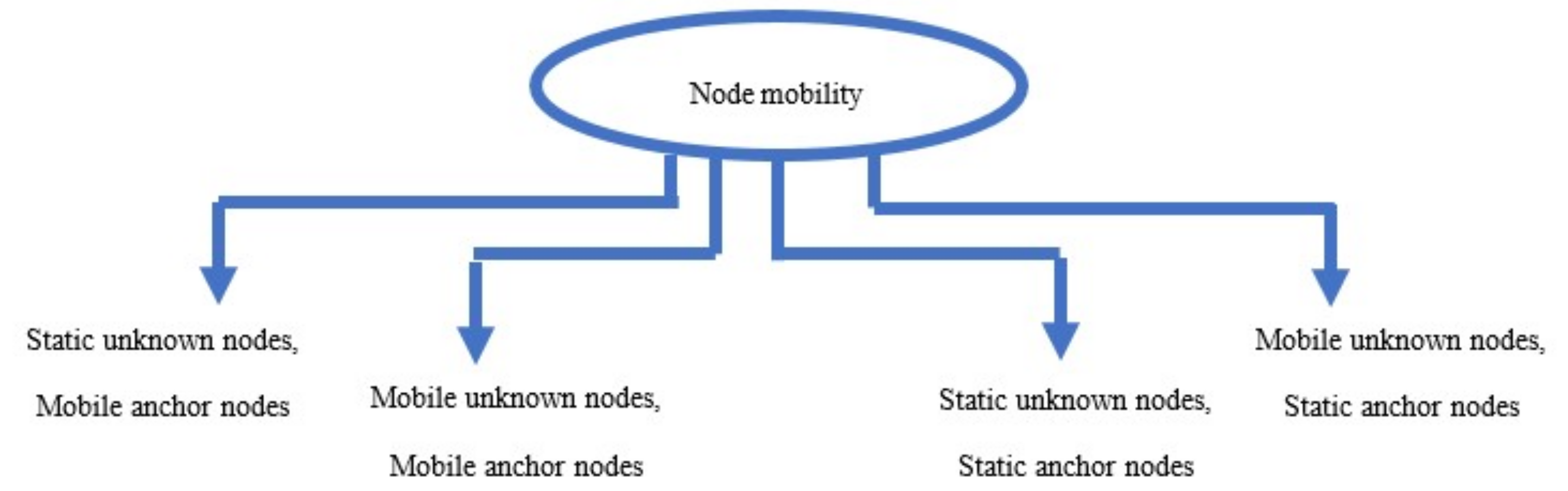
- The unknown nodes are spread in fixed locations.
- Each node has a determined communication range which differs depending on the surrounding criteria.
- The mobile anchor node traverses through the network deterministic path. It can move around any obstacle it meets through its journey.
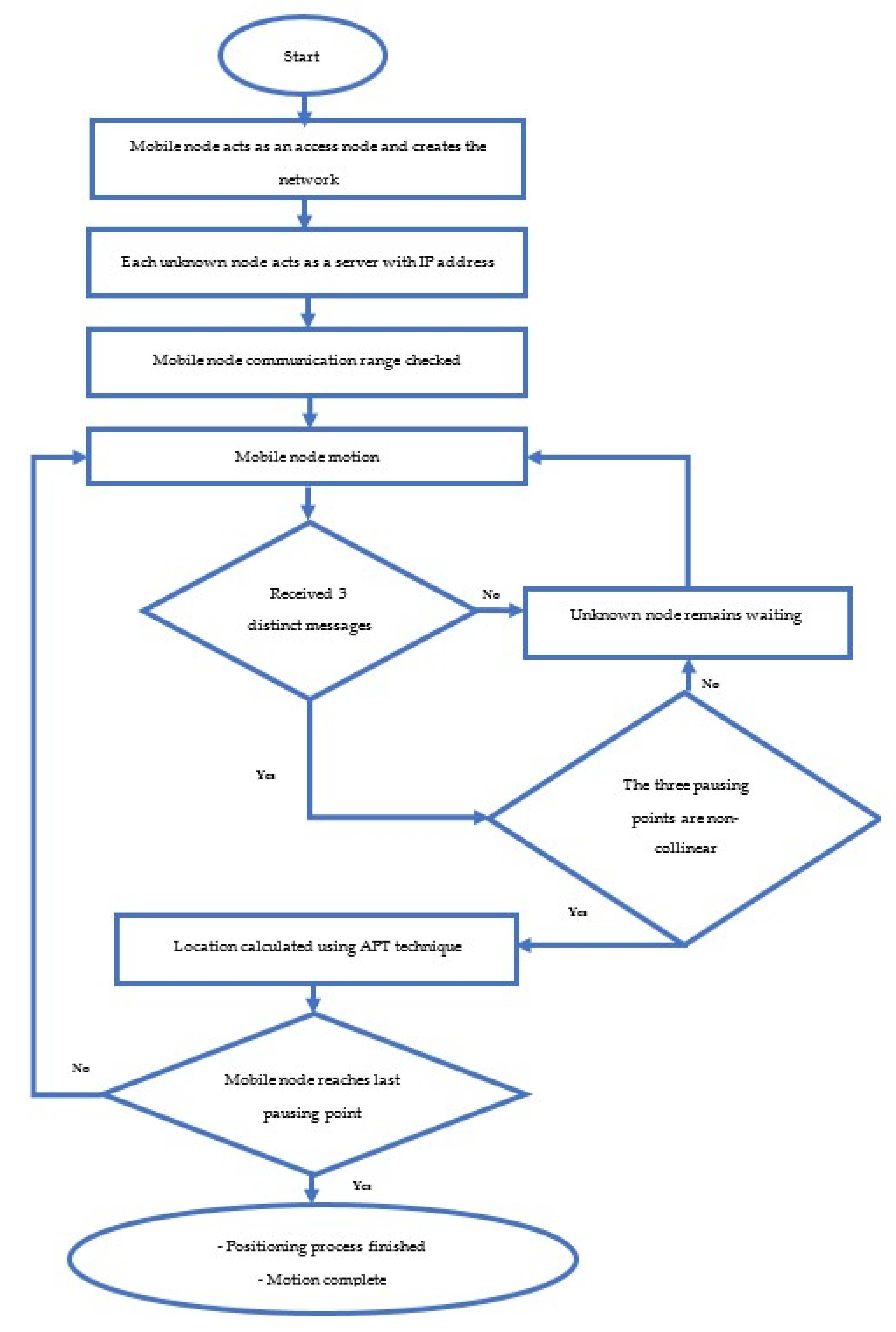
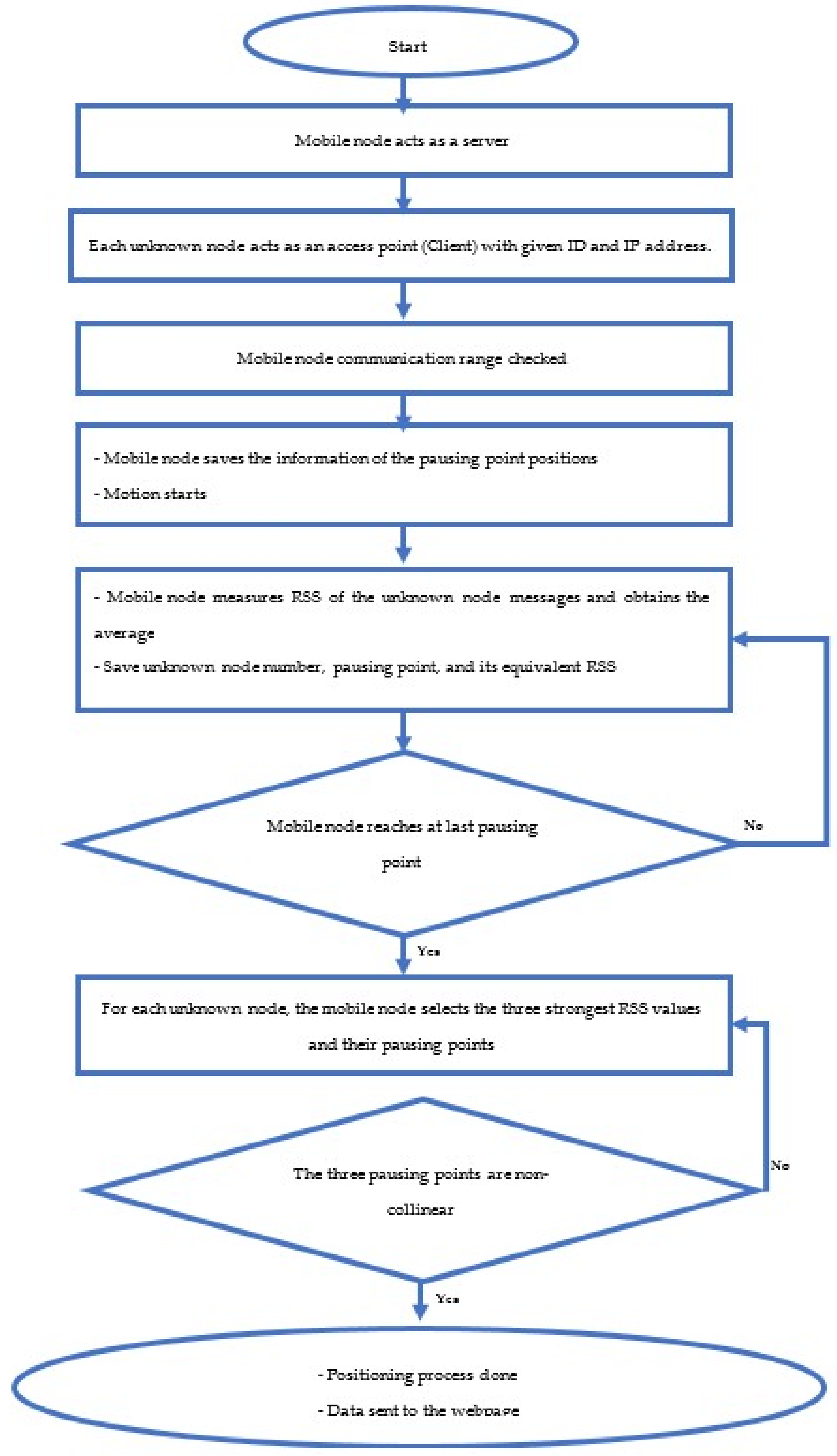
- The mobile anchor sends messages at each pausing point it rests at, and the unknown nodes in its scope receive the messages from it.
- The mobile anchor node can determine its position at each pausing point.
- The unknown node can compute its position via the position information from three different mobile node positions.
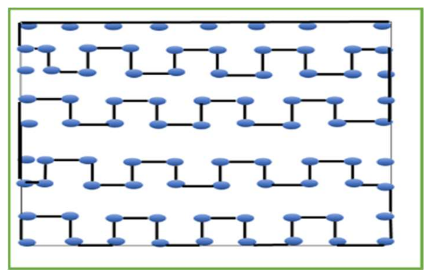
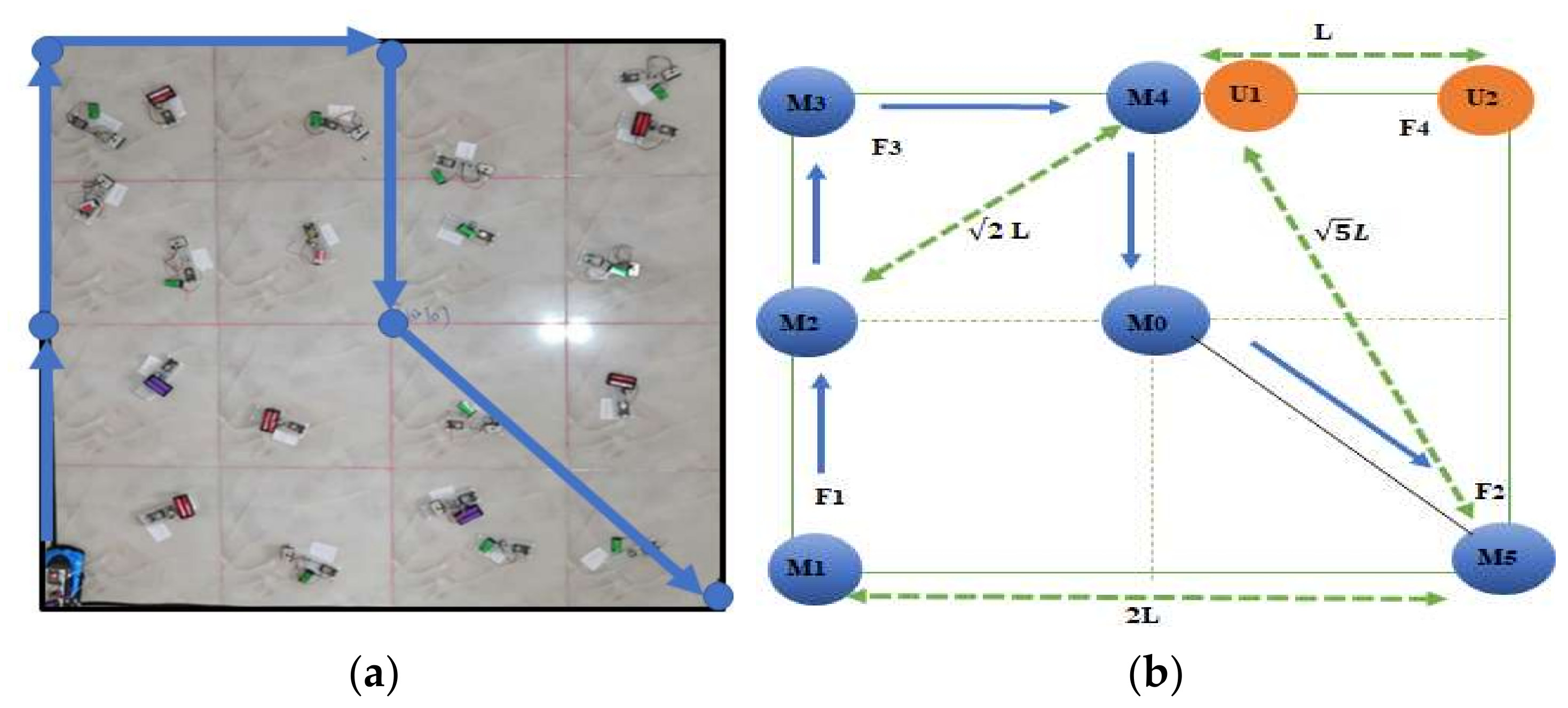
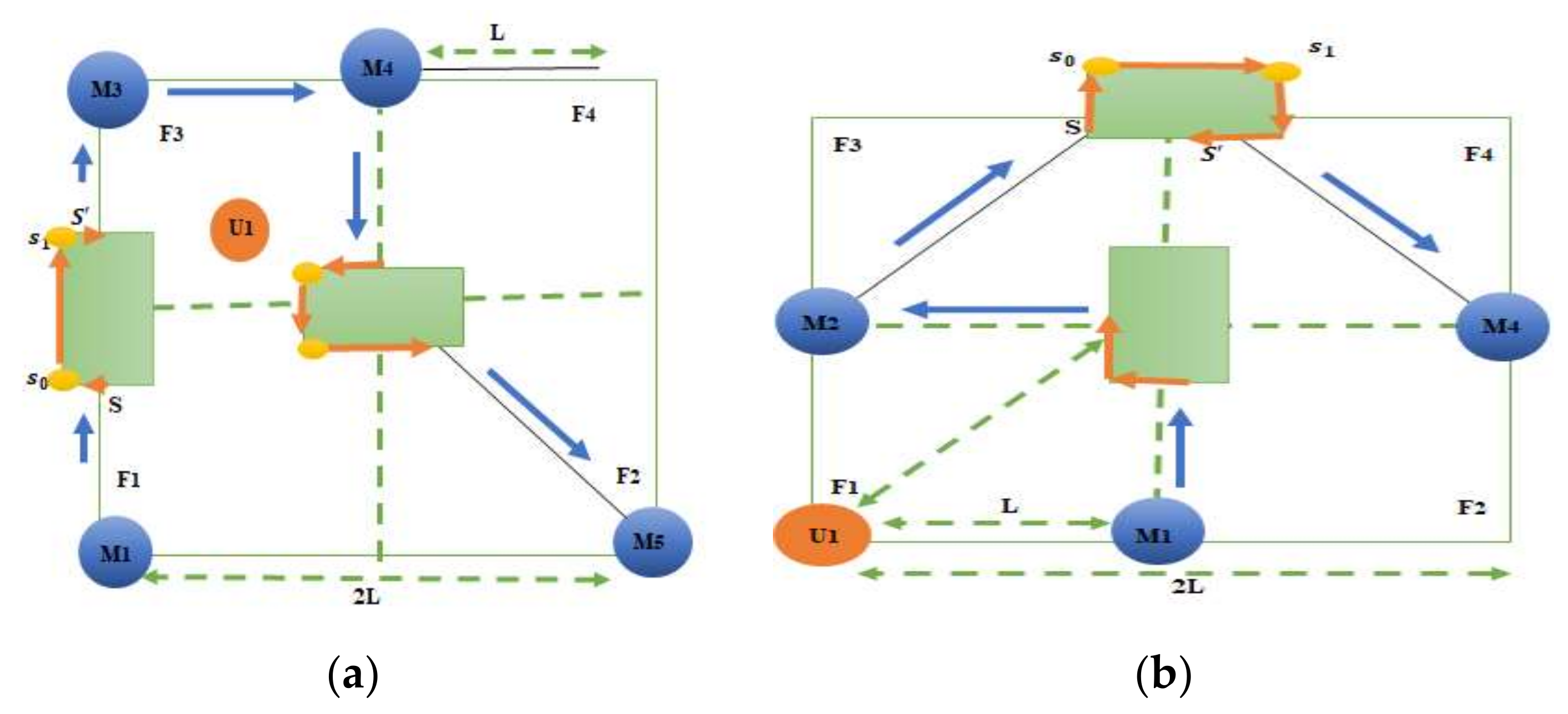
3.1. R-Curve Path Model
3.1.1. Stage 1: Experiment Preparation
3.1.2. Stage 2: Mobility Motion Description
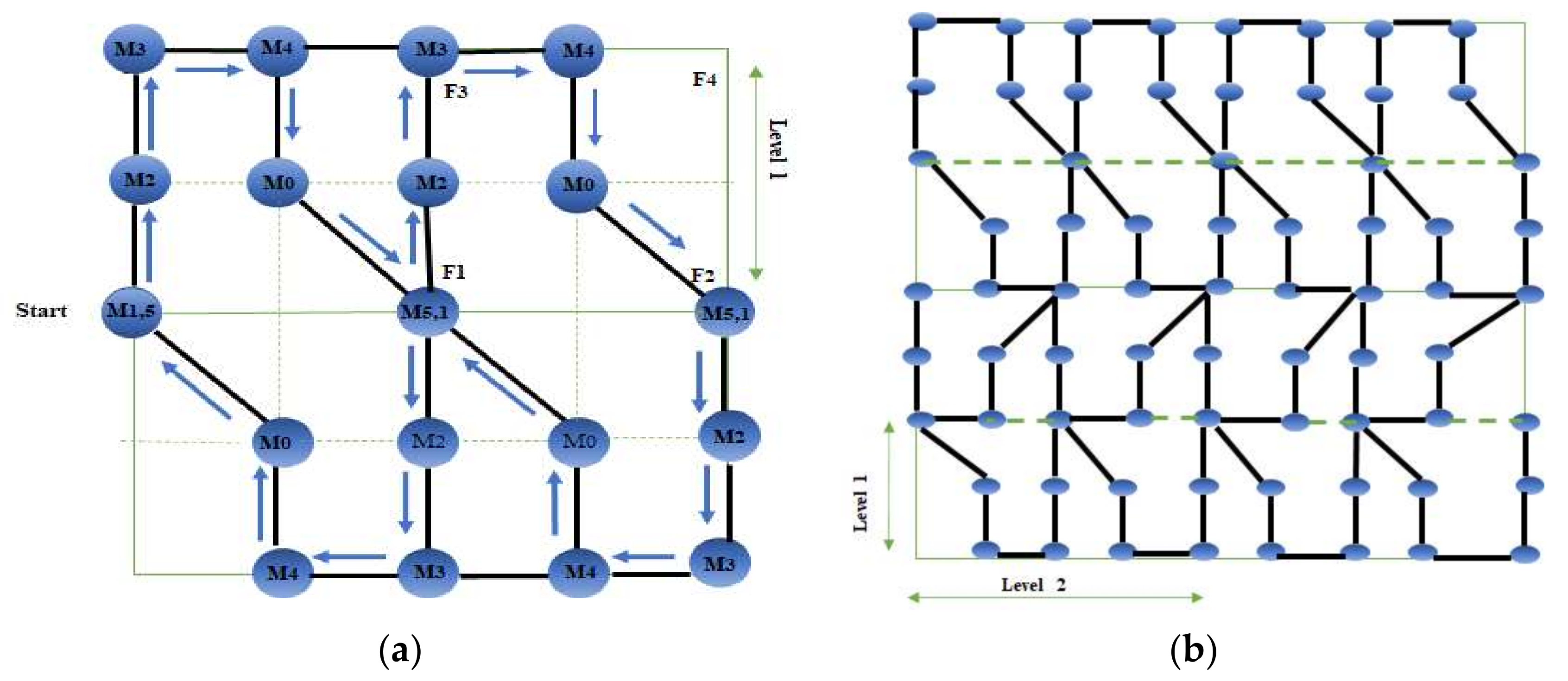
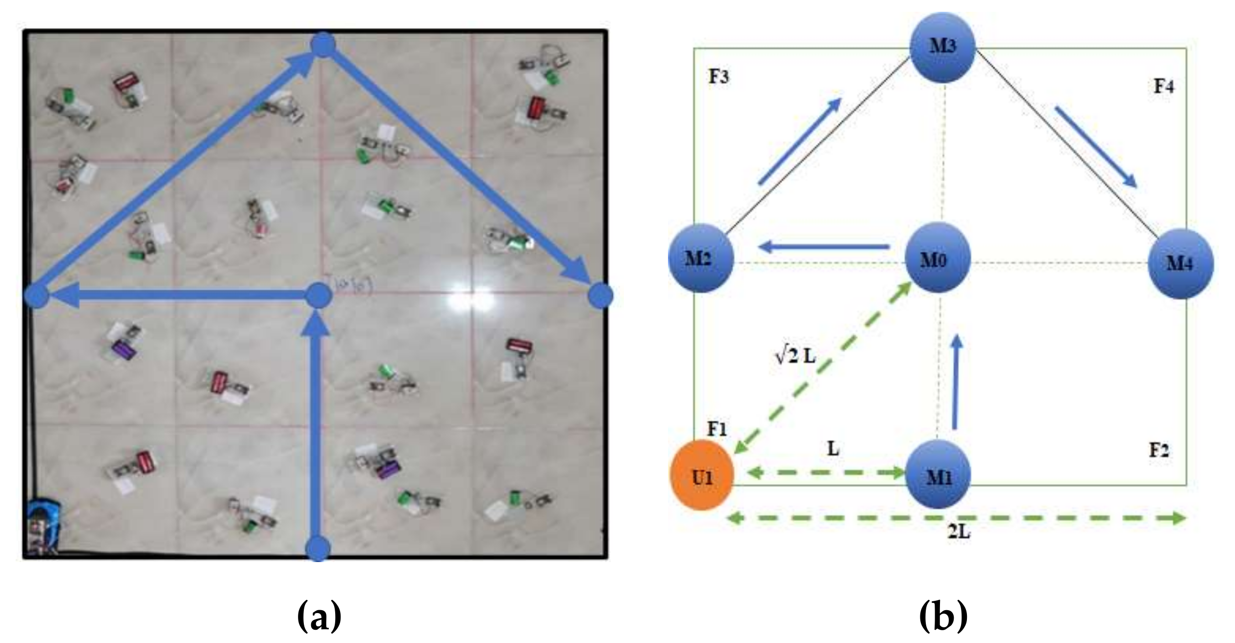
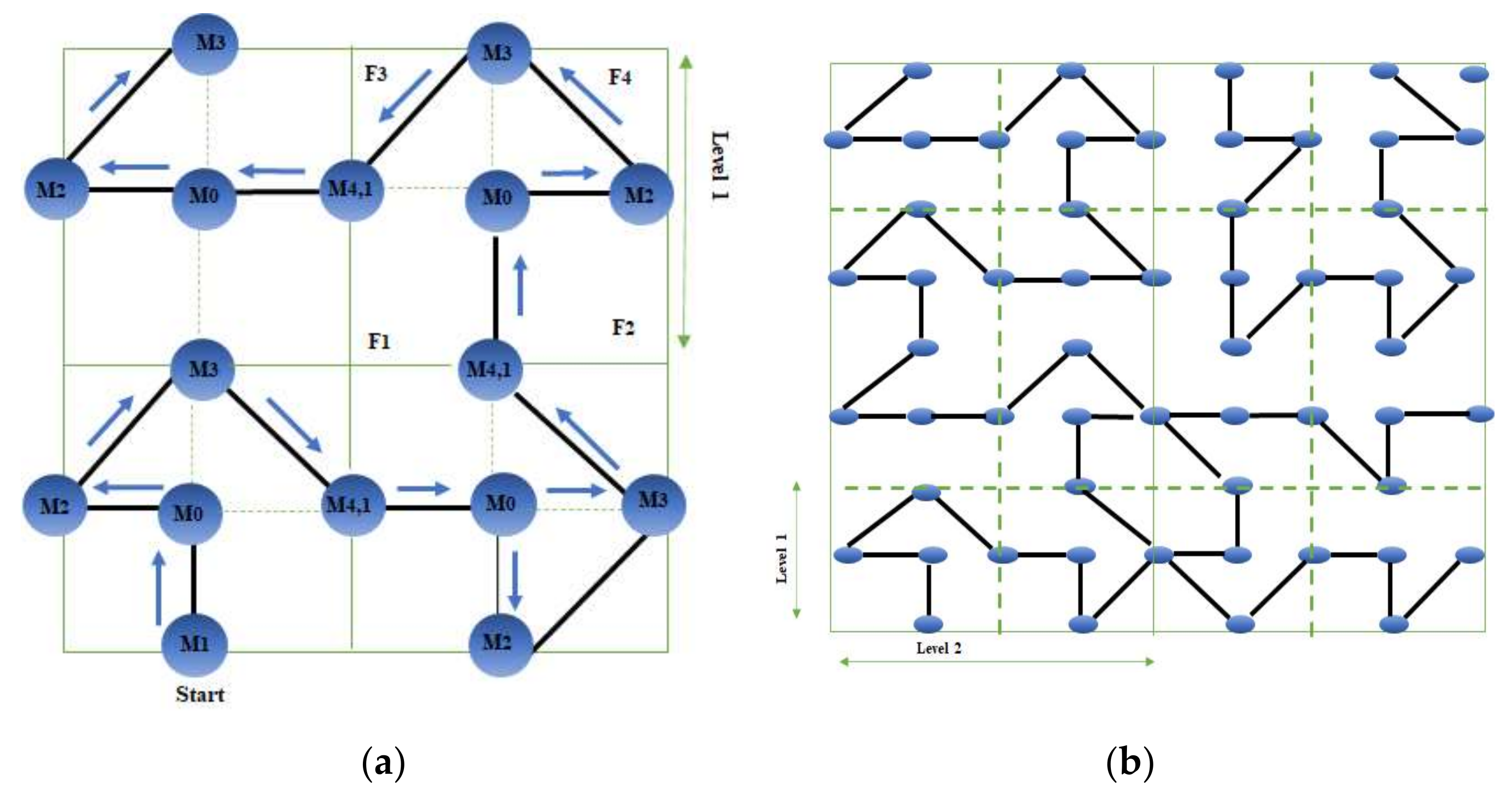
3.2. Arrow-Curve Path Model
Stage 2: Mobility Motion Description
3.3. Obstacle—Reluctant Path
4. Performance Evaluation
4.1. Performance Parameters
- Average localization error.
- 2.
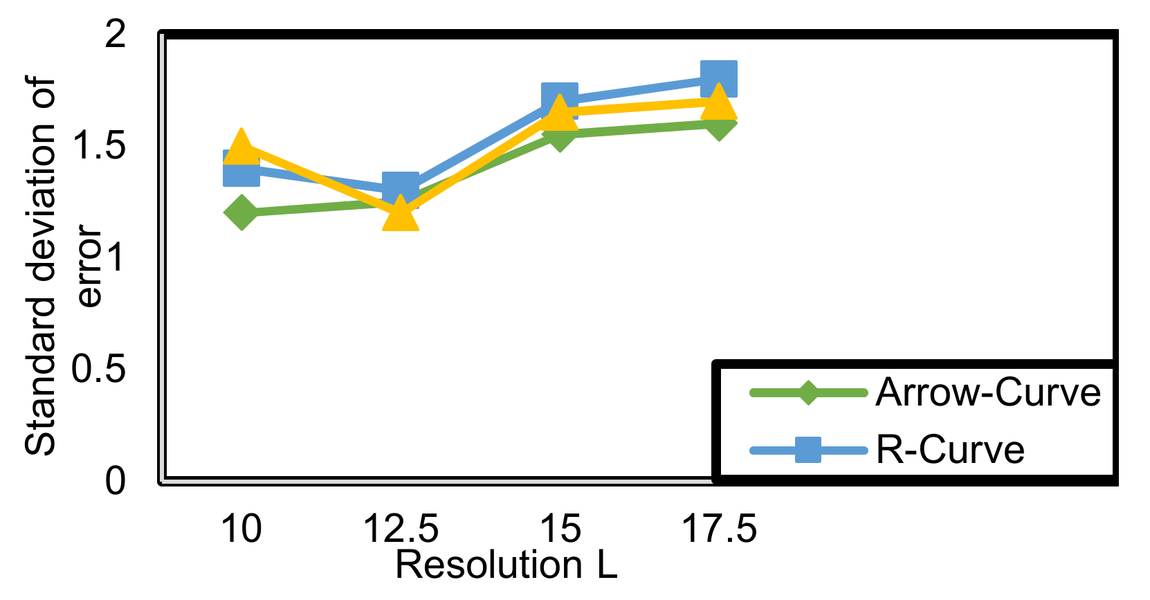
- Standard deviation of position error.
- 3.
- Coverage ratio.
- 4.
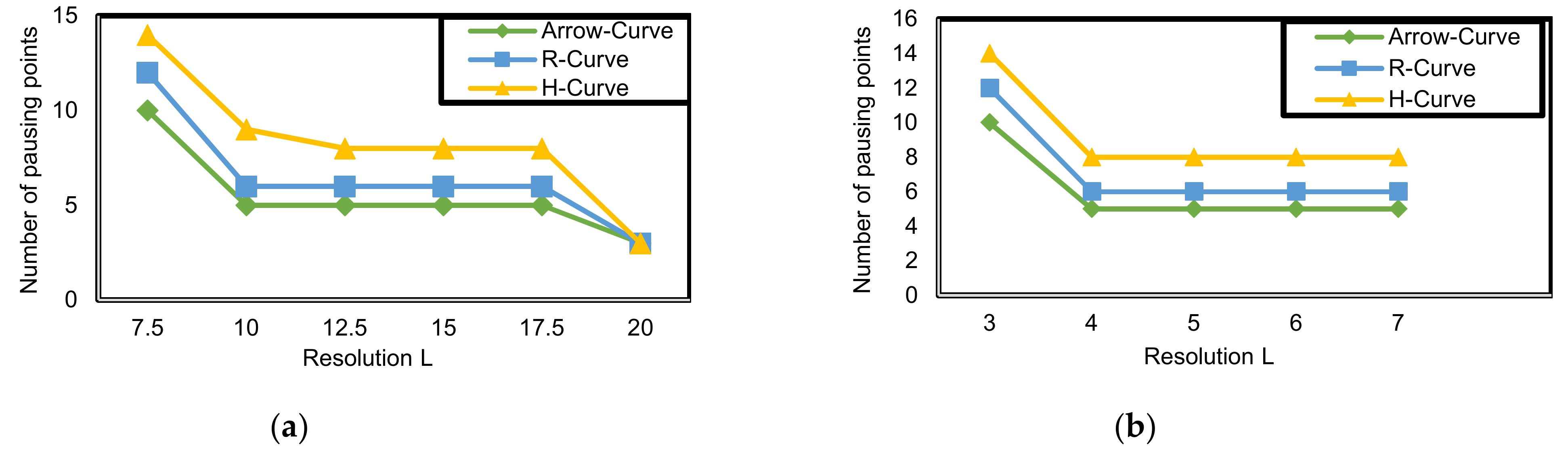
- Number of pausing points.
- 5.
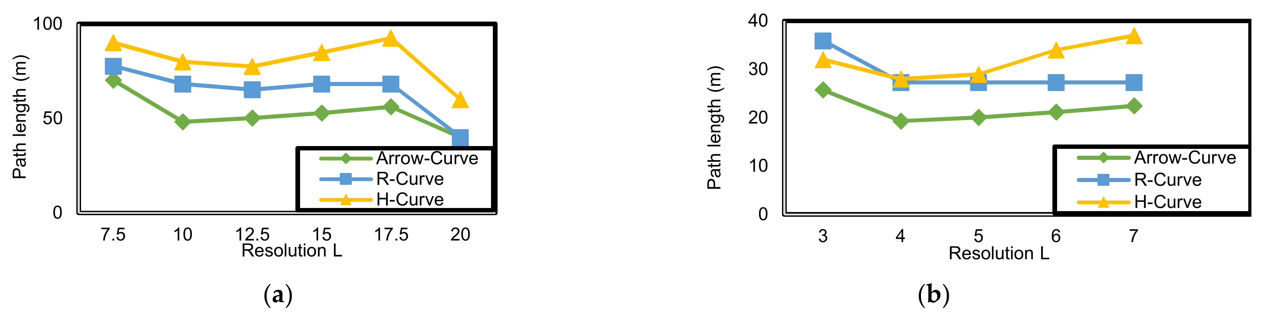
- Path length.
- 6.
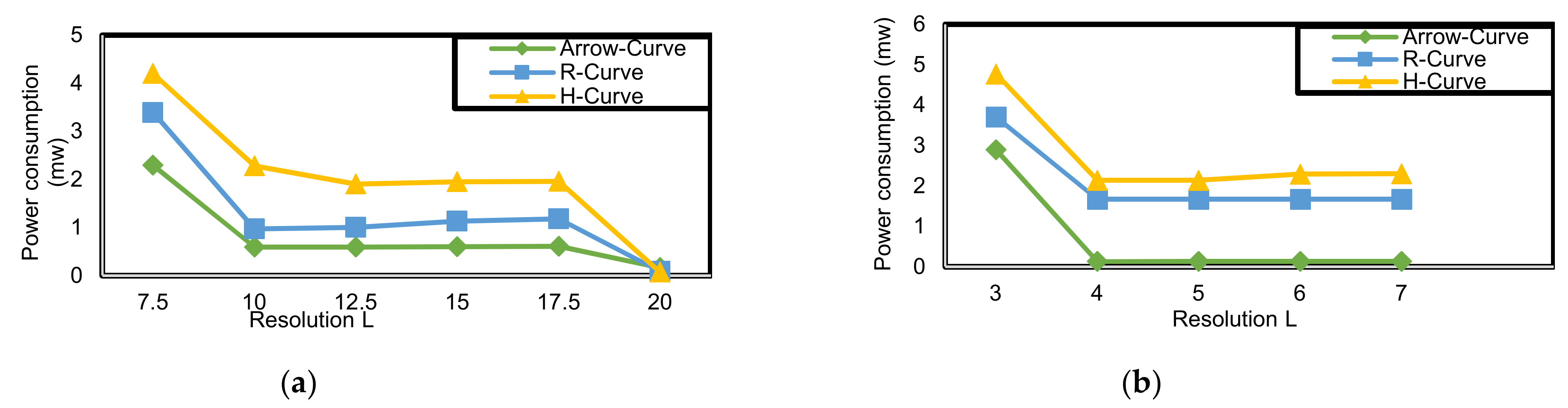
- Energy or power consumption.
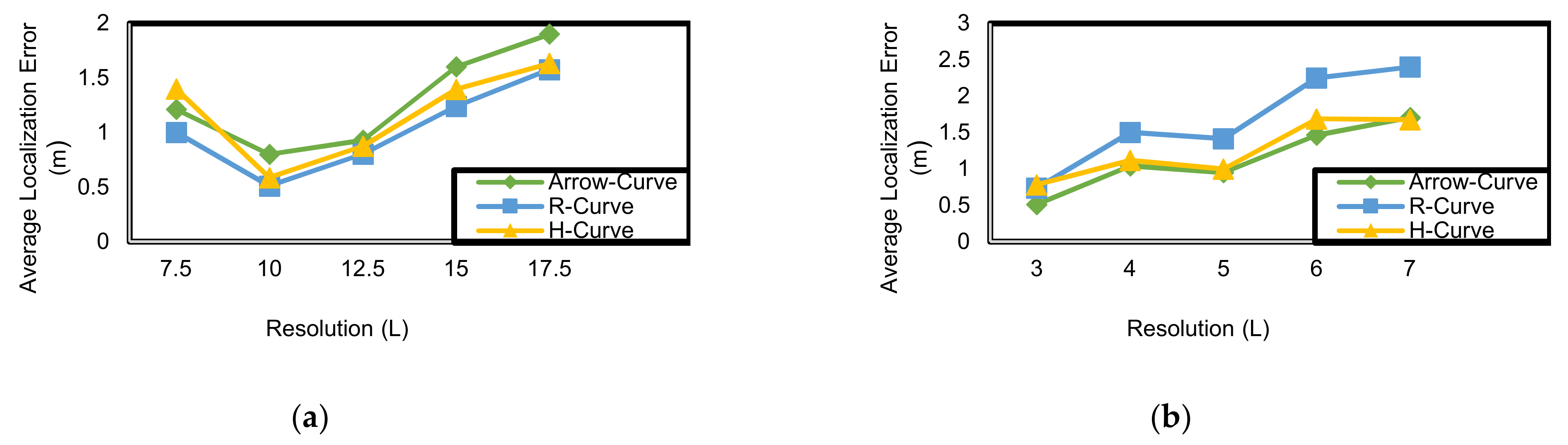
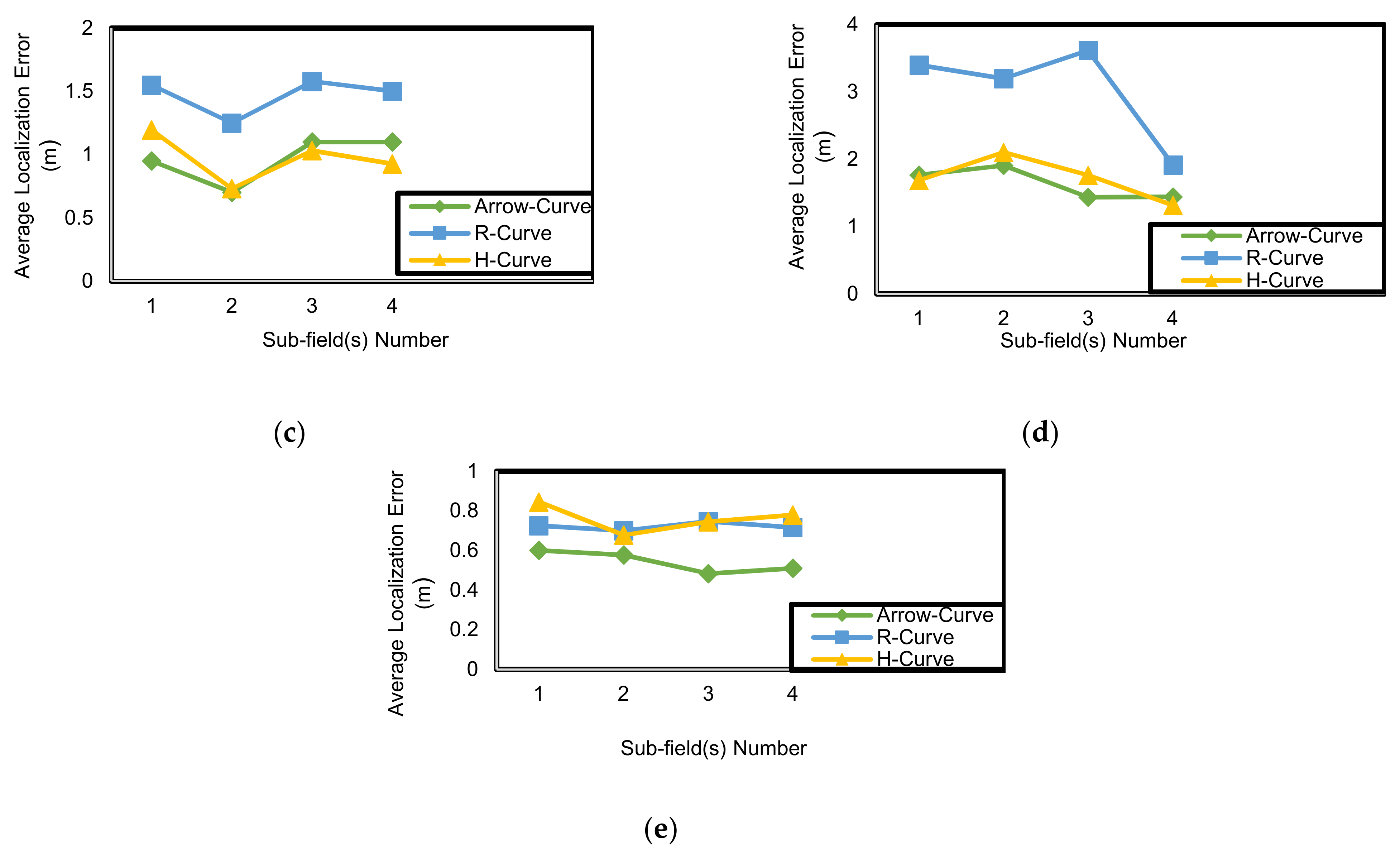
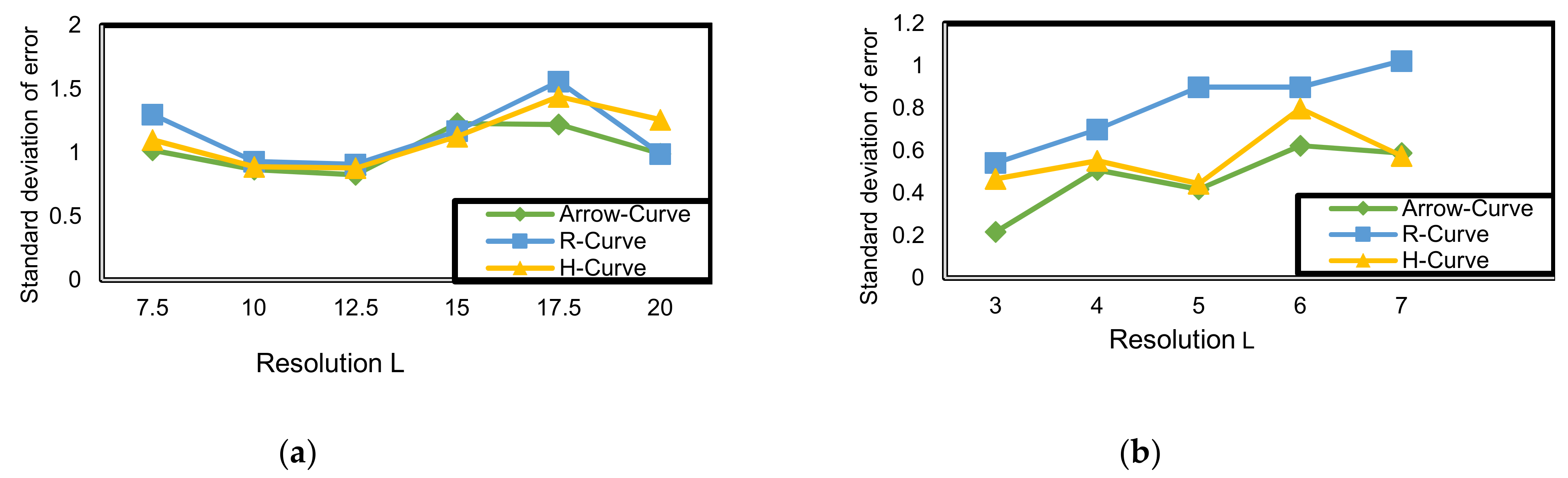
4.2. Performance Evaluation Using MATLAB Simulation
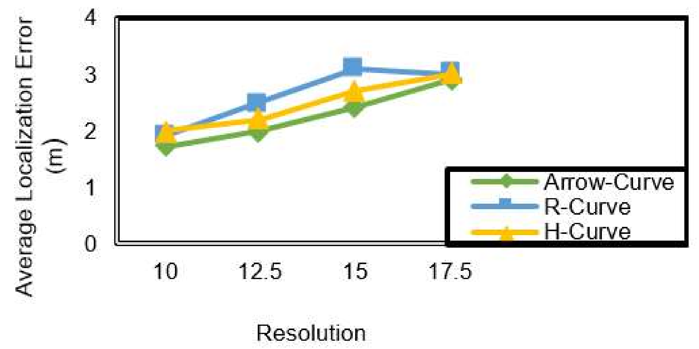
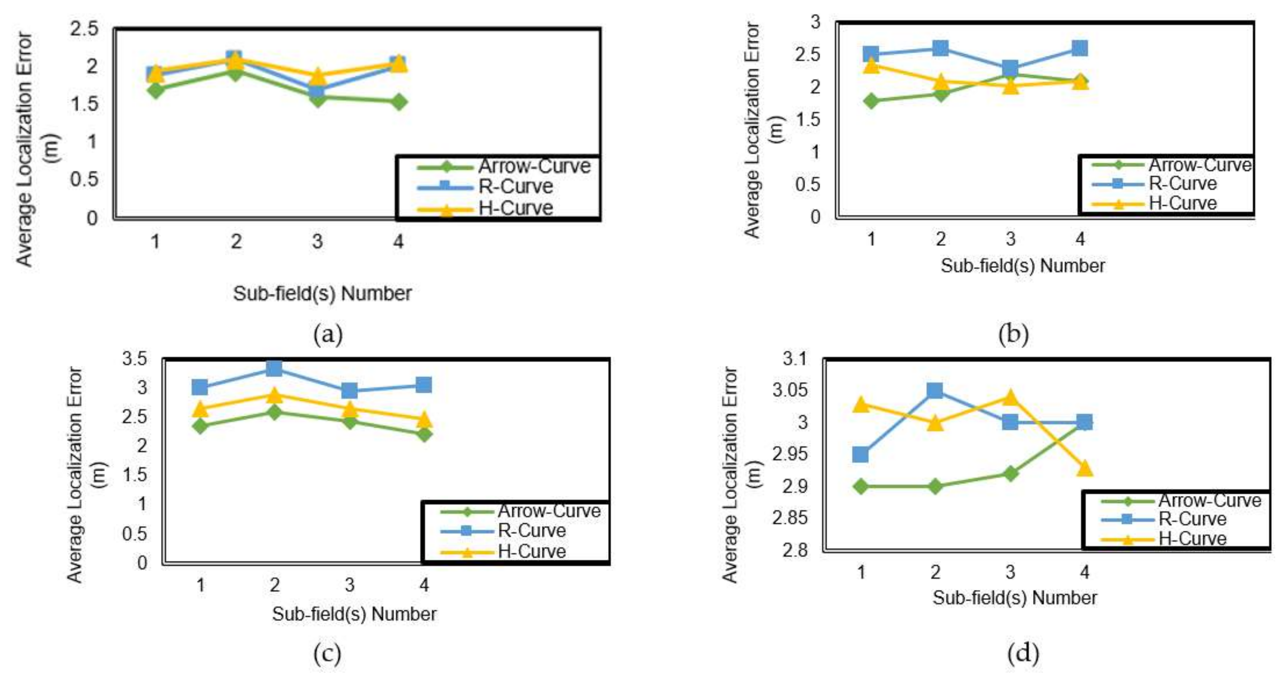
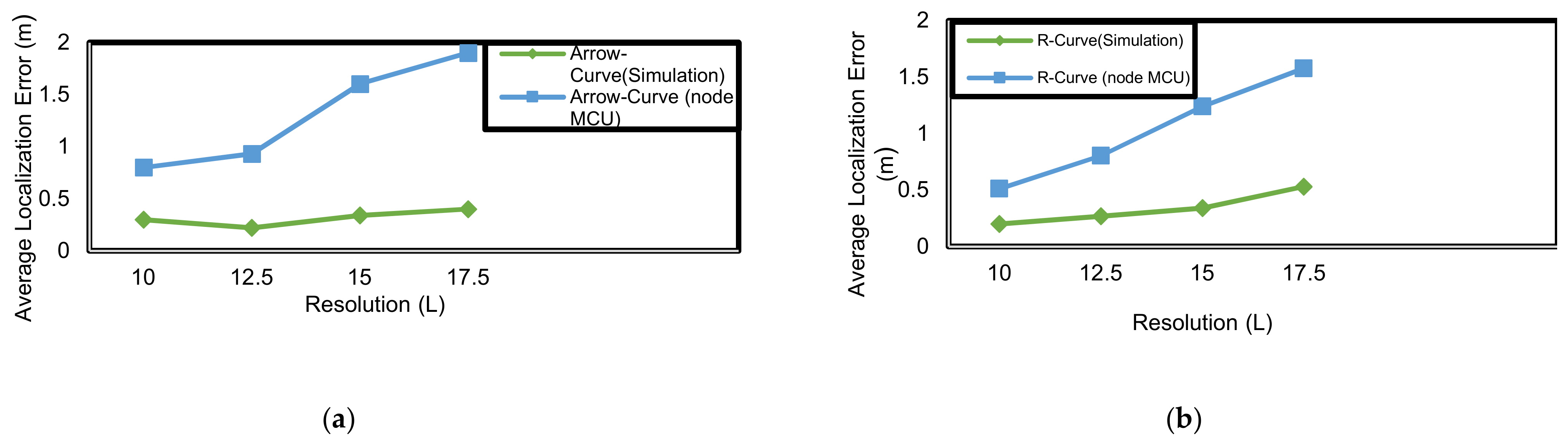
- Average localization error.
- 2.
- Standard deviation of position error.
- 3.
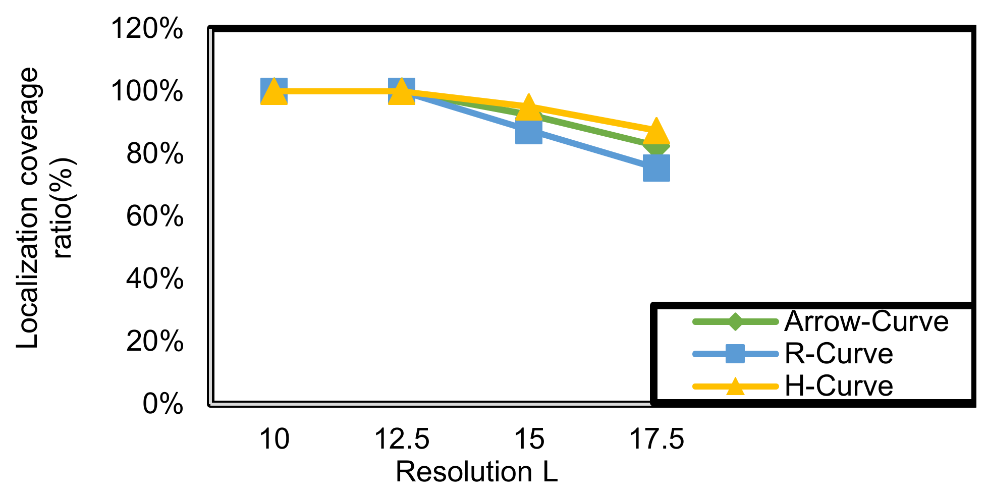
- Coverage ratio.
- 4.
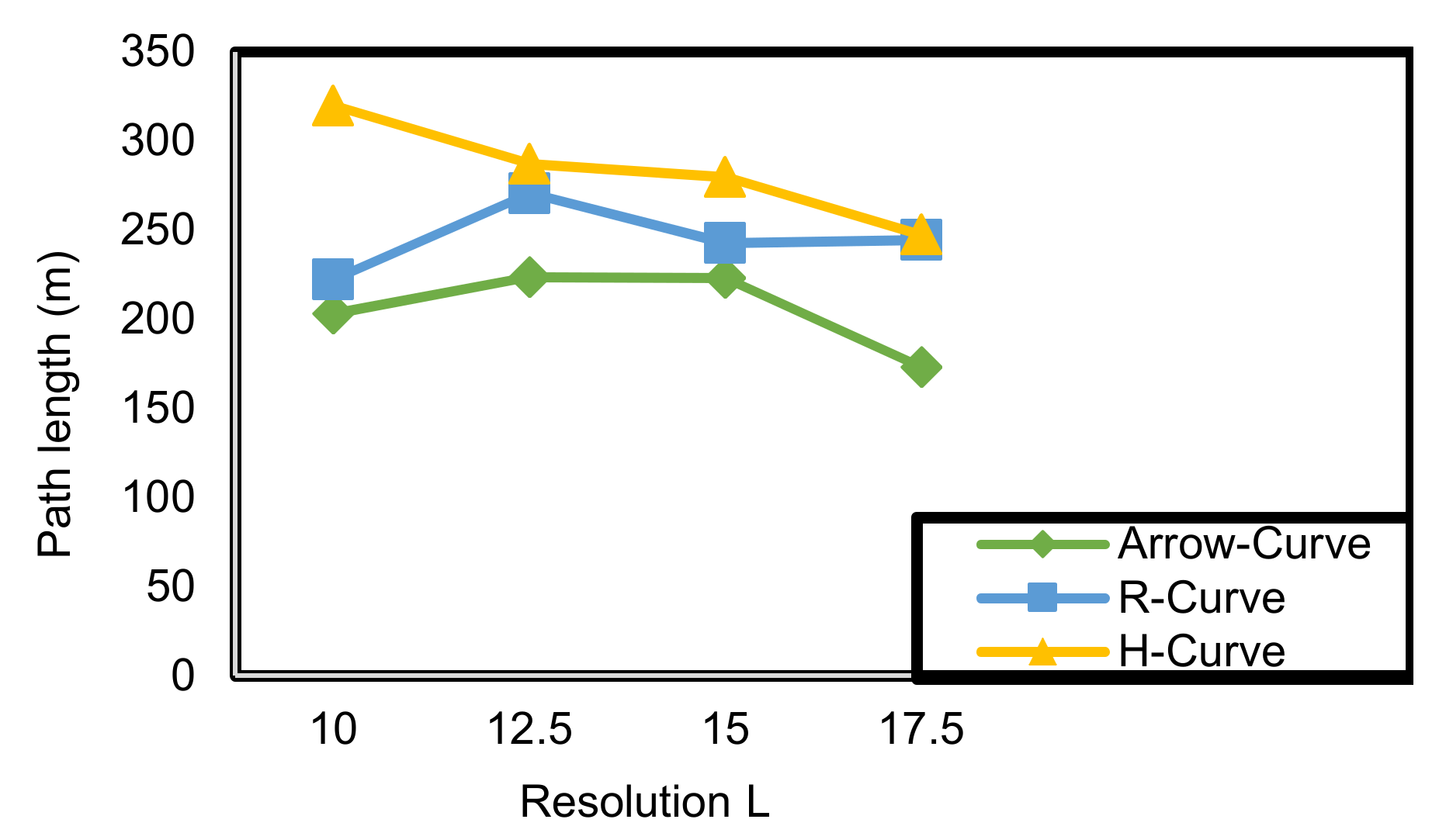
- Path length.
- 5.
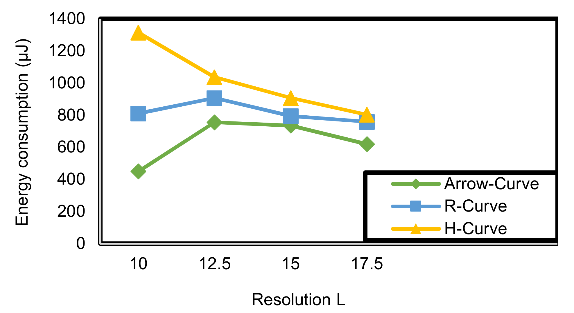
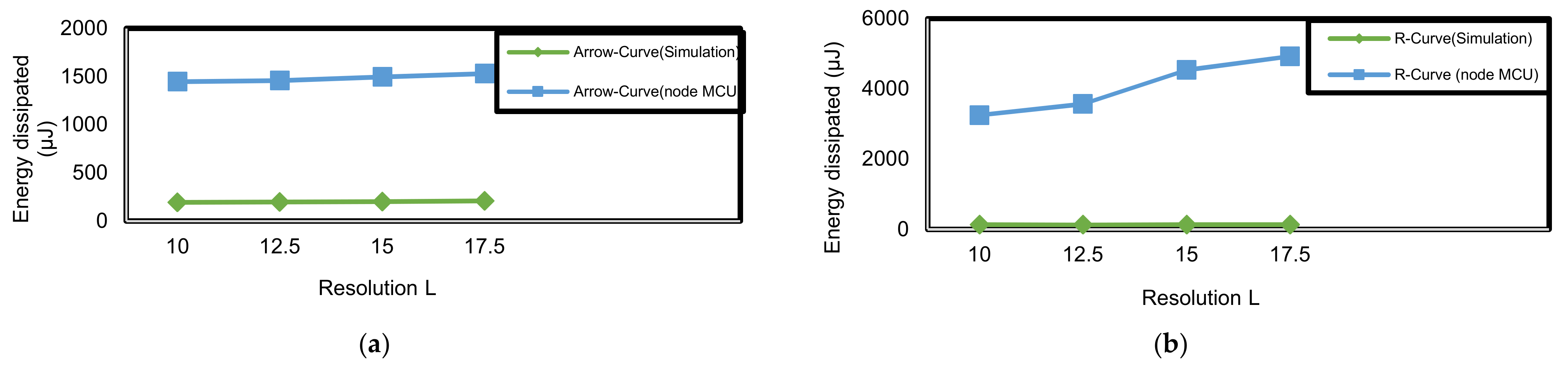
- Energy consumption.
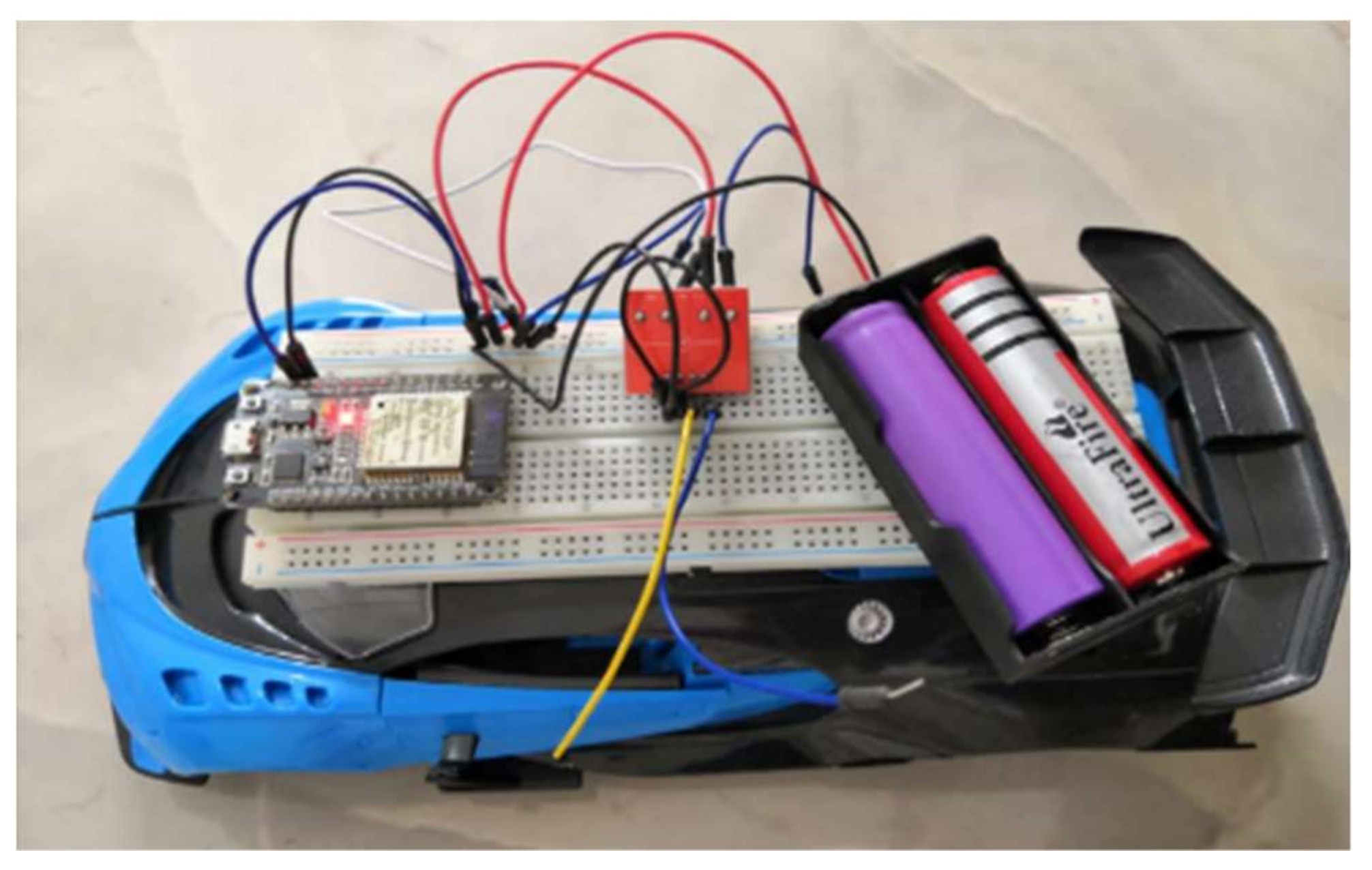
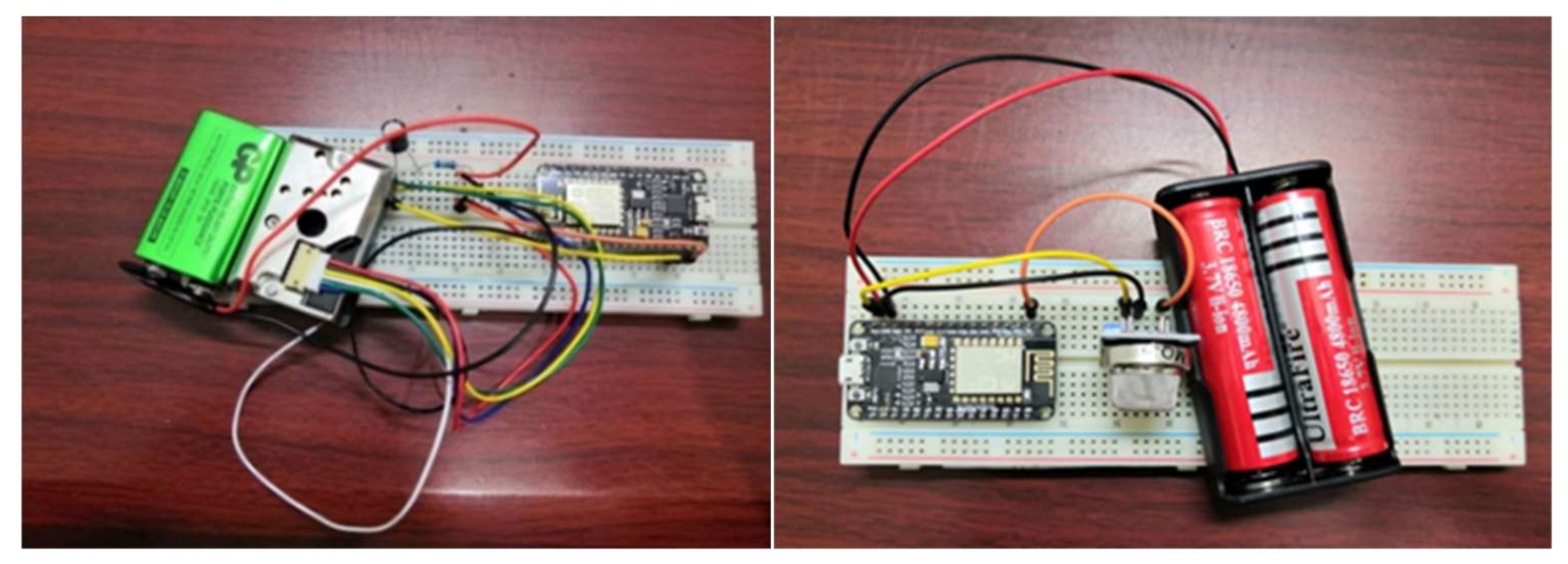
4.3. Performance Evaluation Using Node MCU
- Average localization error.
- 2.
- Standard deviation of position error.
- 3.
- Coverage ratio.
- 4.
- Number of pausing points.
- 5.
- Path length.
- 6.
- Power consumption.
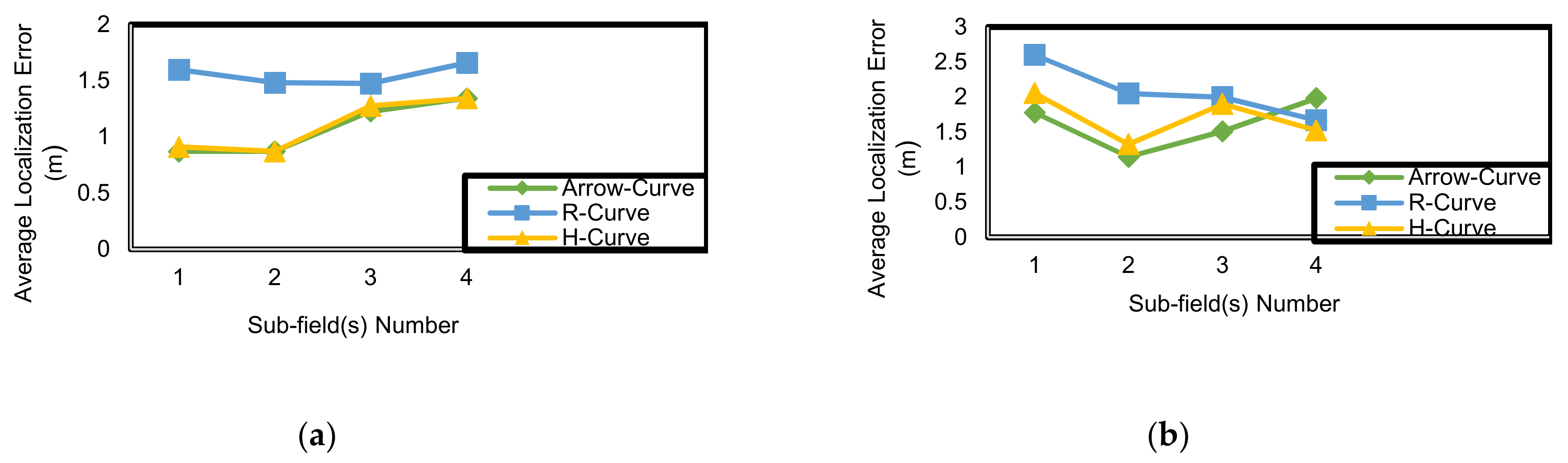
4.4. Performance Evaluation Comparison
- Average localization error
- 2.
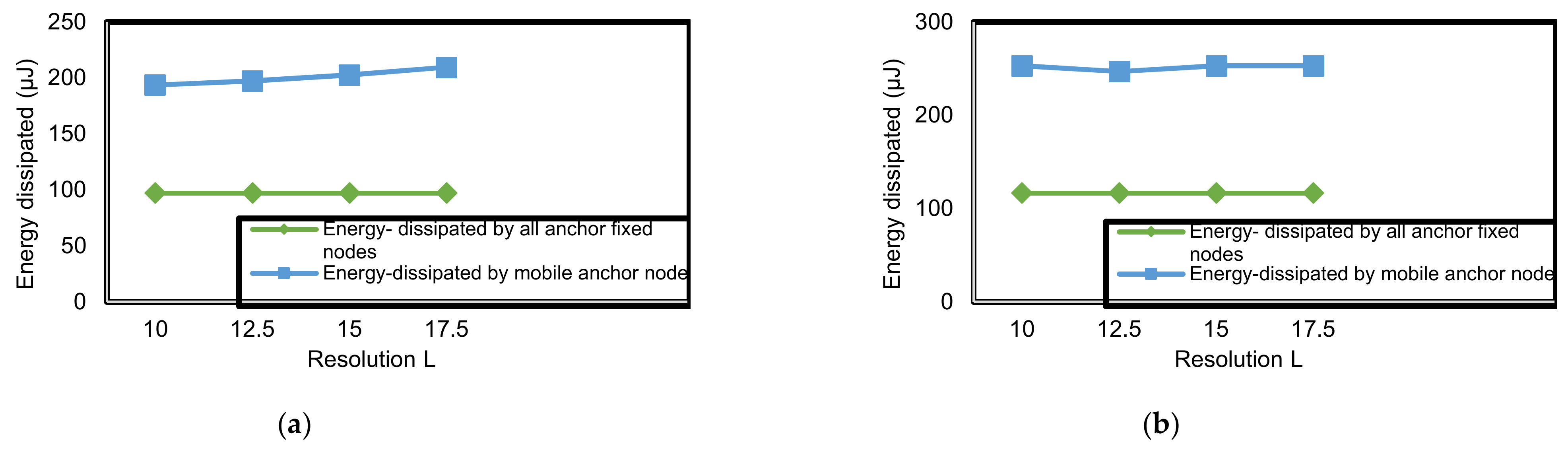
- Energy Consumption
4.5. Replacing One Mobile Anchor Node by Fixed Anchor Nodes
5. Conclusions and Future Work
Author Contributions
Funding
Conflicts of Interest
References
- Mohamed, E.; Zakaria, H.; Abdelhalim, M.B. An improved DV-hop localization algorithm. In Advances in Intelligent Systems and Computing; Springer: Cairo, Egypt, 2017; pp. 332–341. [Google Scholar]
- Rashid, B.; Rehmani, M.H. Applications of wireless sensor networks for urban areas: A survey. J. Netw. Comput. Appl. 2016, 60, 192–219. [Google Scholar] [CrossRef]
- Patwari, N.; Ash, J.N.; Kyperountas, S.; Hero, A.; Moses, R.; Correal, N.S. Locating the nodes: Cooperative localization in wireless sensor networks. IEEE Signal Process. Mag. 2005, 22, 54–69. [Google Scholar] [CrossRef]
- Khelifi, M.; Benyahia, I.; Moussaoui, S.; Nait-Abdesselam, F. An overview of localization algorithms in mobile wireless sensor networks. In Proceedings of the 2015 International Conference on Protocol Engineering (ICPE) and International Conference on New Technologies of Distributed Systems (NTDS), Paris, France, 22–24 July 2015; pp. 1–6. [Google Scholar]
- Bulusu, N.; Heidemann, J.; Estrin, D. GPS-less low-cost outdoor localization for very small devices. IEEE Wirel. Commun. 2000, 7, 28–34. [Google Scholar] [CrossRef] [Green Version]
- Savvides, A.; Han, C.C.; Strivastava, M.B. Dynamic fine-grained localization in Ad-Hoc networks of sensors. In Proceedings of the 7th Annual International Conference on Mobile Computing and Networking, Rome, Italy, 16–21 July 2001; pp. 166–179. [Google Scholar]
- Sichitiu, M.; Ramadurai, V. Localization of wireless sensor networks with a mobile beacon. In Proceedings of the 2004 IEEE International Conference on Mobile Ad-Hoc and Sensor Systems (IEEE Cat. No.04EX975), Fort Lauderdale, FL, USA, 25–27 October 2004; pp. 174–183. [Google Scholar]
- Ssu, K.F.; Ou, C.H.; Jiau, H. Localization with mobile anchor points in wireless sensor networks. IEEE Trans. Veh. Technol. 2005, 54, 1187–1197. [Google Scholar] [CrossRef]
- Lee, S.; Kim, E.; Kim, C.; Kim, K. Localization with a mobile beacon based on geometric constrains in wireless sensor networks. IEEE Wirel. Commun. 2009, 8, 5801–5805. [Google Scholar] [CrossRef]
- Ahmed, E.M.; Hady, A.A.; El-Kader, S.M.A. Optimal path schemes of mobile anchor nodes aided localization for different applications in IoT. In Enabling Machine Learning Applications in Data Science; Springer: Singapore, 2021; pp. 63–76. [Google Scholar]
- Hussein, H.H.; Radwan, M.H.; El-Kader, S.M.A. Proposed localization scenario for autonomous vehicles in GPS denied environment. In Proceedings of the International Conference on Advanced Intelligent Systems and Informatics 2020, Cairo, Egypt, 19–21 October 2020; pp. 608–617. [Google Scholar]
- Ou, C.H.; He, W.L. Path planning algorithm for mobile anchor-based localization in wireless sensor networks. IEEE Sensors J. 2012, 13, 466–475. [Google Scholar] [CrossRef]
- Priyantha, N.B.; Chakraborty, A.; Balakrishnan, H. The Cricket location-support system. In Proceedings of the 6th Annual International Conference on Mobile Computing and Networking, Boston, MA, USA, 6–11 August 2000; pp. 32–43. [Google Scholar]
- Bahi, P.; Padmarrabhan, V.N. RADAR: An in-building RF- based user location and tracking system. In Proceedings of the IEEE INFOCOM 2000. Conference on Computer Communications. Nineteenth Annual Joint Conference of the IEEE Computer and Communications Societies, Tel Aviv, Israel, 26–30 March 2000; pp. 775–784. [Google Scholar]
- Niculescu, D.; Nath, B. Ad hoc positioning system (APS) using AOA. In Proceedings of the IEEE INFOCOM 2003. Twenty-Second Annual Joint Conference of the IEEE Computer and Communications Societies (IEEE Cat. No. 03CH37428), San Francisco, CA, USA, 30 March–3 April 2003; Volume 3, pp. 1734–1743. [Google Scholar]
- He, T.; Huang, C.; Blum, B.M.; Stankovic, J.A.; Abdelzaher, T. Range-free localization schemes for large scale sensor networks. In Proceedings of the MobiCom03: Ninth Annual International Conference on Mobile Computing and Networking, San Diego, CA, USA, 14–19 September 2003; pp. 81–95. [Google Scholar]
- Niculescu, D.; Nath, B. DV-based positioning in ad hoc networks. Telecommun. Syst. 2003, 22, 267–280. [Google Scholar] [CrossRef]
- Mao, G.; Fidan, B.; Anderson, B.D. Wireless sensor network localization techniques. Comput. Netw. 2007, 51, 2529–2553. [Google Scholar] [CrossRef] [Green Version]
- Han, G.; Xu, H.; Duong, T.Q.; Jiang, J.; Hara, T. Localization algorithms of wireless sensor networks: A survey. Telecommun. Syst. 2013, 52, 2419–2436. [Google Scholar] [CrossRef]
- Patwari, N.; Hero, I.A.; Perkins, M.; Correal, N.; O’Dea, R. Relative location estimation in wireless sensor networks. IEEE Trans. Signal Process. 2003, 51, 2137–2148. [Google Scholar] [CrossRef] [Green Version]
- Nourhan, A.N.; Hossam, F.; Hady, A.A. The enhanced probability hypothesis density-based filter for multitarget tracking and counting. In Proceedings of the 2019 Novel Intelligent and Leading Emerging Sciences Conference (NILES), Giza, Egypt, 28–30 October 2019; pp. 92–97. [Google Scholar]
- Chen, H.; Shi, Q.; Tan, R.; Poor, H.V.; Sezaki, K. Mobile element assisted cooperative localization for wireless sensor networks with obstacles. IEEE Trans. Wirel. Commun. 2010, 9, 956–963. [Google Scholar] [CrossRef]
- Guo, Z.; Guo, Y.; Hong, F.; Jin, Z.; He, Y.; Feng, Y.; Liu, Y. Perpendicular intersection: Locating wireless sensors with mobile beacon. IEEE Trans. Veh. Technol. 2010, 59, 3501–3509. [Google Scholar] [CrossRef]
- Ou, C.H. A localization scheme for wireless sensor networks using mobile anchors with directional antennas. IEEE Sensors J. 2011, 11, 1607–1616. [Google Scholar] [CrossRef]
- Rezazadeh, J.; Moradi, M.; Ismail, A.S. Efficient localization via Middle-node cooperation in wireless sensor networks. In Proceedings of the International Conference on Electrical, Control and Computer Engineering 2011 (InECCE), Kuantan, Malaysia, 21–22 June 2011; pp. 410–415. [Google Scholar]
- Ahmed, E.M.; Hady, A.A.; El-Kader, S.A.; Khalil, A.; Mahmoud, A. Localization methods for internet of things: Current and future trends. In Proceedings of the 2019 6th International Conference on Advanced Control Circuits and Systems (ACCS) & 2019 5th International Conference on New Paradigms in Electronics & Information Technology (PEIT), Hurgada, Egypt, 17–20 November 2019; pp. 119–125. [Google Scholar]
- Abo-Elhassab, A.E.; Abd El-Kader, S.M.; Elramly, S. Wireless Sensor Networks Localization, Routing Protocols and Architectural Solutions for Optimal Wireless Networks and Security; IGI Global: Hershey, PA, USA, 2017; pp. 204–240. [Google Scholar]
- Baggio, L.K. Monte Carlo localization for mobile sensor networks. Ad Hoc Netw. 2008, 6, 718–733. [Google Scholar] [CrossRef]
- Hu, L.; Evans, D. Localization for mobile sensor networks. In Proceedings of the 10th Annual International Conference on Mobile Computing and Networking, Philadelphia, PA, USA, 26 September–1 October 2004; pp. 45–57. [Google Scholar]
- Koutsonikolas, D.; Das, S.M.; Hu, Y.C. Path planning of mobile landmarks for localization in wireless sensor networks. In Proceedings of the 26th IEEE International Conference on Distributed Computing Systems Workshops (ICDCSW’06), Lisboa, Portugal, 4–7 July 2006. [Google Scholar]
- Han, G.; Xu, H.; Jiang, J.; Shu, L.; Hara, T.; Nishio, S. Path planning using a mobile anchor node based on trilateration in wireless sensor networks. Wirel. Commun. Mob. Comput. 2013, 13, 1324–1336. [Google Scholar] [CrossRef]
- Rezazadeh, J.; Moradi, M.; Ismail, A.S.; Dutkiewicz, E. Superior path planning mechanism for mobile beacon-assisted localization in wireless sensor networks. IEEE Sensors J. 2014, 14, 3052–3064. [Google Scholar] [CrossRef]
- Alomari, C.F.; Phillips, W.; Aslam, N. New path planning model for mobile anchor assisted localization in wireless sensor Networks. Wirel. Netw. 2018, 24, 2589–2607. [Google Scholar] [CrossRef]
- Chang, C.Y.; Sheu, J.P.; Chen, Y.C.; Chang, S.W. An obstacle-free and power-efficient deployment algorithm for wireless sensor networks. IEEE Trans. Syst. Man, Cybern.-Part A Syst. Humans 2009, 39, 795–806. [Google Scholar] [CrossRef]
- MATLAB. Available online: https://www.mathworks.com/products/matlab.html (accessed on 14 October 2021).
- Rezazadeh, J.; Moradi, M.; Ismail, A.S.; Dutkiewicz, E. Impact of static trajectories on localization in wireless sensor networks. Wirel. Netw. 2014, 21, 809–827. [Google Scholar] [CrossRef]
- ESP32. Available online: https://www.espressif.com/en/products/socs/es32 (accessed on 1 October 2020).
- ESP8266. Available online: https://www.espressif.com/en/products/socs/esp8266 (accessed on 1 October 2020).
- Datasheet. Available online: https://www.sparkfun.com/datasheets/Sensors/gp2y1010au_e.pdf (accessed on 29 October 2021).
- Datasheet. Available online: https://datasheetspdf.com/pdf/622943/Hanwei/MQ-2/1 (accessed on 29 October 2021).
- Software Arduino. Available online: https://www.arduino.cc/en/software (accessed on 1 November 2020).


| Parameter | Value |
|---|---|
| Network area size | 50 × 50 |
| Number of mobile anchor nodes | 1 |
| Number of unknown nodes | 40 |
| Resolution L | L = 10, 12.5, 15, 17.5 |
| Path loss exponent () | 3.3 |
| ( | −59 |
| 1 m | |
| Standard deviation of noise (σ) | 4 |
| Communication range | 15 |
| Simulation run times | 10 |
| Parameter | Value |
|---|---|
| Network area size | 20 × 20 (outdoor); 8 × 8 (indoor) |
| Number of mobile anchor nodes | 1 |
| Number of unknown nodes | 20 (outdoor); 10 (indoor) |
| Resolution L | L = 20, 17.5, 15, 12.5, 10, 7.5 (outdoor); L = 8, 7, 6, 5, 4, 3 (indoor) |
| Path loss exponent () | 2.3 (outdoor); 5.2 (indoor) |
| ( | −54. |
| 0.4 m | |
| Number of beacons received at each pausing point. | 50 |
| Communication range | 28 m outdoor; 9 m indoor with obstacles |
| Parameter | Value |
|---|---|
| Network area size | 20 × 20 |
| Number of mobile anchor nodes | 1 |
| Number of unknown nodes | 20 (outdoor) |
| Resolution L | L = 10, 12.5, 15, 17.5, |
| Path loss exponent () | 2.3 |
| ( | −54 |
| 0.4 m | |
| Number of beacons received at each pausing point (Node MCU) | 50 |
| Simulation run times (MATLAB) | 10 |
| Communication range | 28 m |
Publisher’s Note: MDPI stays neutral with regard to jurisdictional claims in published maps and institutional affiliations. |
© 2021 by the authors. Licensee MDPI, Basel, Switzerland. This article is an open access article distributed under the terms and conditions of the Creative Commons Attribution (CC BY) license (https://creativecommons.org/licenses/by/4.0/).
Share and Cite
Ahmed, E.M.; Hady, A.A.; El-Kader, S.M.A.; Khalil, A.T.; Mohamed, W.A. An Arrow-Curve Path Planning Model for Mobile Beacon Node Aided Localization in Air Pollution Monitoring System IoT. Electronics 2021, 10, 2757. https://doi.org/10.3390/electronics10222757
Ahmed EM, Hady AA, El-Kader SMA, Khalil AT, Mohamed WA. An Arrow-Curve Path Planning Model for Mobile Beacon Node Aided Localization in Air Pollution Monitoring System IoT. Electronics. 2021; 10(22):2757. https://doi.org/10.3390/electronics10222757
Chicago/Turabian StyleAhmed, Enas M., Anar A. Hady, Sherine M. Abd El-Kader, Abeer Twakol Khalil, and Wael A. Mohamed. 2021. "An Arrow-Curve Path Planning Model for Mobile Beacon Node Aided Localization in Air Pollution Monitoring System IoT" Electronics 10, no. 22: 2757. https://doi.org/10.3390/electronics10222757
APA StyleAhmed, E. M., Hady, A. A., El-Kader, S. M. A., Khalil, A. T., & Mohamed, W. A. (2021). An Arrow-Curve Path Planning Model for Mobile Beacon Node Aided Localization in Air Pollution Monitoring System IoT. Electronics, 10(22), 2757. https://doi.org/10.3390/electronics10222757