Raymarching Distance Fields with CUDA

Abstract

Raymarching is a technique for rendering implicit surfaces using signed distance fields. It has been known and used since the 1980s for rendering fractals and CSG (constructive solid geometry) surfaces, but has rarely been used for commercial rendering applications such as film and 3D games. Raymarching was first used for photorealistic rendering in the mid 2000s by demoscene developers and hobbyist graphics programmers, receiving little to no attention from the academic community and professional graphics engineers. In the present work, we explain why the use of Simple and Fast Multimedia Library (SFML) by nearly all existing approaches leads to a number of inefficiencies, and hence set out to develop a CUDA oriented approach instead. We next show that the usual data handling pipeline leads to further unnecessary data flow overheads and therefore propose a novel pipeline structure that eliminates much of redundancy in the manner in which data are processed and passed. We proceed to introduce a series of data structures which were designed with the specific aim of exploiting the pipeline’s strengths in terms of efficiency while achieving a high degree of photorealism, as well as the accompanying models and optimizations that ultimately result in an engine which is capable of photorealistic and real-time rendering on complex scenes and arbitrary objects. Lastly, the effectiveness of our framework is demonstrated in a series of experiments which compare our engine both in terms of visual fidelity and computational efficiency with the leading commercial and open source solutions, namely Unreal Engine and Blender.

1. Introduction

The focus of the present work is the development of a realtime 3D rendering engine using Raymarching in CUDA and the optimization techniques required to improve the processing and memory costs compared to conventional rendering techniques so that it can be used without case specific tuning on complex scenes while maintaining a high degree of photorealism.

Raymarching (also known as sphere tracing) is a technique which can be used to determine the intersection of a ray with an implicit surface by marching a ray through a distance field [1,2]. Given a point in space, a ray, and a signed distance function (SDF) for the distance between a point in space and the closest intersection with geometry in the scene, an iterative march ray forward through the scene is done until a surface is intersected or a predicate for ray termination met. Unlike ray tracing, which requires exact analytical intersection functions, it is possible to use SDFs of non exact geometry such as fractals, procedurally generated isosurfaces, volumetric textures, heightmaps, as well as typical analytical surfaces (primitives such as spheres, triangles, cubes, etc.). This extra flexibility makes raymarching highly attractive.

However, raymarching is rarely used in industry as a technique for rendering surfaces and has instead been adopted and developed by hobbyists. One such example would be in demoscene, where raymarching is a popular technique used to render everything from vast landscapes to simple structures where often the entire raymarching pipeline sits in a single fragment shader making it remarkably lightweight and viable for less performant platforms.

In this paper, we introduce a series of contributions. Firstly, we analyse relevant previous work, both in the published academic literature and the non-published open source realm, and argue that the existing approaches’ nearly universal adoption of the SFML (Simple and Fast Multimedia Library) leads to wastefulness and inefficiency. Hence, we make a case for a CUDA oriented approach instead. Within this context, we next show that the commonly employed data handling pipeline leads to further unnecessary data flow overheads and therefore introduce a novel pipeline that eliminates much of the observed data redundancy. To make the most out of the new pipeline, we next proceed to describe a series of data structures which were developed with the specific aim of exploiting the pipeline’s strengths in terms of efficiency while requiring visually high performant solutions (i.e., a high degree of photorealism), as well as the accompanying models and optimizations that ultimately result in an engine which is capable of photorealistic and real-time rendering on complex scenes and arbitrary objects. Its performance is demonstrated and analysed thereafter.

Related Work and Context

Raymarching is a technique for rendering implicit surfaces using geometric distance. Given a signed distance function (SDF) returning the distance to an object from a given point in space, sphere-tracing marches along a ray towards the closest intersection point of the surface iteratively. This technique can be used to find intersections with a variety of surfaces including fractals, procedurally generated isosurfaces, volumetric textures, heightmaps, as well as typical analytical surfaces.

Raymarching was first described by Hart et al. in 1989 [1] and was used to render 3D Julia sets. The paper laid the foundations for the technique and discussed issues such as minimum ray incrementation with thin surfaces, avoiding bad distance estimates with bounding volumes, and maximum ray incrementation, as well as methods to calculate surface normals. The original implementation of raymarching was specific to fractals and did not explore other surface types in depth. The subsequent work by Hart [2] explored raymarching in much more depth with the focus being on the technique itself as opposed to its specific application for fractal rendering. This paper established conventions in raymarching which largely persist to this day.

The next significant advancement in raymarching development was made by Quilez [3] whose 4 kilobyte raymarcher was capable of rendering a complex, realistic scene in near real time. Quilez discussed the pros and cons of ray marching distance fields and demonstrated techniques unique to distance field rendering such as arbitrary combination and instantiation of objects, infinite repetition, space deformation, surface detailing and shape blending. It is the first work which discusses lighting in raymarched scenes.

Quilez can be credited as person who introduced raymarching to the demoscene community, with his “Making a simple apple with maths” raymarcher [4] being the most forked code on the glsl.heroku OpenGL sandbox, and Shadertoy, co-developed by Quilez, now hosts numerous self-contained raymarching shaders. Quilez’s website [5] also contains dozens of articles on raymarching which are considered as the de facto reference for construction of raymarching shaders.

Raymarching offers a number of benefits as compared with ray tracing and rasterization, some of which are:

• Compactness. As we noted already, raymarching is highly lightweight both in size of codebase and memory footprint. A raymarcher can be contained entirely in a fragment shader program and can be executed on a variety of hardware and platforms such as WebGL, OpenGL ES, and OpenGL.
• Performance. Raymarching is an excellent approximation for ray-tracing, making it a lightweight solution for determining geometry intersection in a rendering pipeline. Raymarching also approximates cone-tracing which makes it a lightweight solution for direct and indirect lighting computation.
• Quality. Since raymarching can ‘emulate’ a ray-tracing pipeline, it is possible to achieve the same level of photorealism as ray-tracing which has become the standard for high-fidelity offline rendering. Raymarching can take advantage of existing anti-aliasing techniques such as MSAA (multisample anti-aliasing), PPAA (post-processing antialiasing) and TAA (temporal anti-aliasing), as well as supporting interpolation based anti-aliasing similar to sub-pixel AA used by 2D font rasterizers for decades without the need of multi-sampling.

Modern raymarchers tend to be entirely self contained in a single fragment shader which is drawn onto a rectangle. OpenGL is usually used as the backend to set up a simple scene onto which the raymarched scenes are projected onto; this makes GLSL the obvious choice for the fragment shader program. However, GLSL operates at a very high level and OpenGL gives very little control on how the program itself is run on the GPU, which makes optimisation difficult and can result in unavoidable divergence between GPU threads when computed. An alternative is to use OpenGL as the backend for projection and texture management, but perform raymarching itself using a different technology with finer grain control over the computation; OpenCL and CUDA are both excellent choices which support OpenGL interoperability. Using a compute-focused language for real-time raymarching has not been explored yet. Granskog explored raymarching with CUDA [6] with the focus being offline rendering as opposed to real time, whereas Keeter [7] described real-time rendering of implicit surfaces with CUDA and OpenGL using a technique orthogonal to raymarching. Granskog’s engine is fairly primitive compared with that which we develop in the present paper and is only be able to deal with simple colouring of surfaces and multibounce lighting. Keeter, on the other hand, unlike us, makes scene specific assumptions, making his work not applicable to real-time performance on general scenes, again in contrast to the engine we introduce.

To summarize previous work and contextualize our contribution, there are two types of CUDA ray marchers: real-time but achieving minimal photorealism (e.g., Granskog’s [6]), and non-realtime but implementing photorealistic light transport (e.g., using offline renderers). The approach we introduce in the the present achieves real-time rendering with photorealistic results which has only been done previously using GLSL shaders (for example, Quilez’s WebGL shaders) or within limited scope and practicability experiments using high level shaders (Cg in Unity or shader graphs in Unreal) for just some parts of a mostly rasterized scene. The closest work to ours is Code Parade’s ‘Marble Marcher’ GLSL based game (https://codeparade.itch.io/marblemarcher accessed on 4 November 2021) which is highly limited by its fractal focus, and restricted in photorealism and the type of scenes it can handle in real time. What sets CUDA apart from GLSL, and what makes the framework developed in the present paper significant, is how closely married it is to many features of the C++ language such as dynamic allocation, the use of function pointers, and templating which opens many more possibilities for a unified graphics pipeline, whereas prior GLSL approaches would require a new shader to be made to change the scene in ways that could not be achieved through simple parameterisation.

2. Proposed Framework

For both rasterization and ray tracing engines, there are multiple pipeline architectures, all with different strengths and weaknesses. However, raymarching is largely unexplored territory in this regard. The pipeline developed herein is summarized in Figure 1. Unlike most graphical engines, the render pipeline for this engine resides mostly on the graphics card, eliminating one of the bottlenecks present in many graphics engines: data transfer and API calls from host to device.

In a typical raster engine data such as textures, meshes and shader code are uploaded and cached in device VRAM (video random access memory), but the model that controls how these data are assembled in a 3D world is completely controlled by the host. The host assembles all this data with what are known as “draw calls”. A draw call itself often consists of multiple API commands, such as binding textures, switching shader programs or specifying vertex buffers. A bottleneck occurs when the host issues commands faster than the device can complete the work. One solution to this would be batching large amounts of work into a single call, known as instancing; for example, draw calls in a loop where only some parameters change between each iteration can be replaced by a single draw call that also takes a list of the precomputed parameters for all instances in an array. Instancing only works in cases where only minor parameters are changed between each instance, such as object transforms or more abstract parameters used by shaders. Instancing, however, is not suitable to render different types of objects: it would not be possible to batch draw calls corresponding to drawing a tree with draw calls corresponding to a table, or in cases where the objects require different shaders or different buffers to be bound.

Our engine has no concept of draw calls which eliminates the CPU bottleneck totally. Instead of issuing commands which need to be processed by the graphics driver, the engine instead uploads arrays of parameters in batches directly from host memory into device memory on the GPU which the model uses to generate the scene. The model itself is defined in device code, in contrast to a raster engine where the application model is defined by the commands issued by host code.

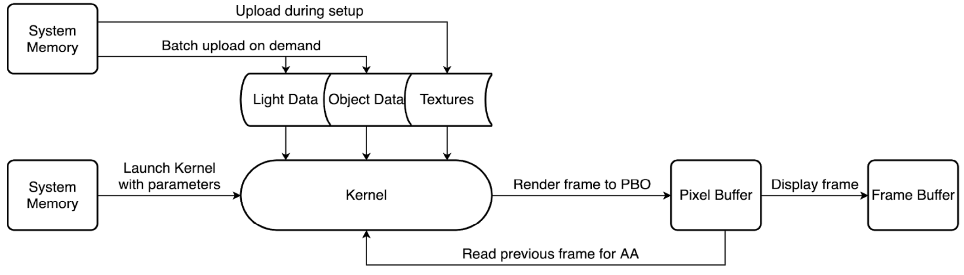
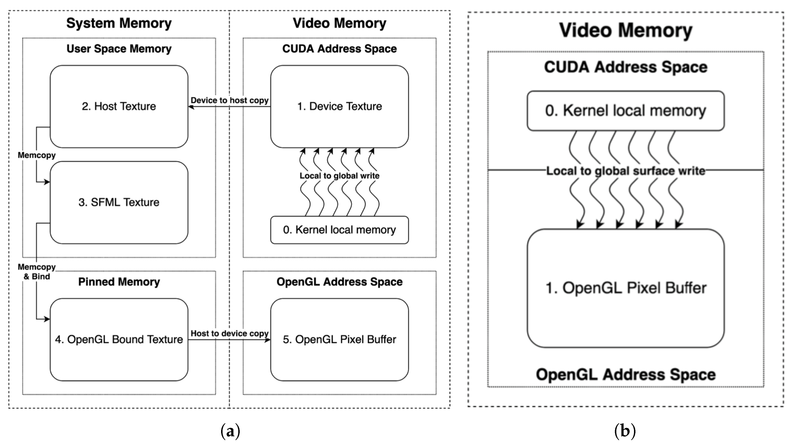
2.1. OpenGL (Open Graphics Library) and CUDA Interoperability

By itself, CUDA kernels have no way of interfacing with a render target or display context, making real-time rendering using only the CUDA API not possible. To overcome this issue, the data produced by the kernel (in this case, a 2D image texture written to by the kernel) must be copied from a CUDA device address space to some address space that the display driver can access.

The first solution that we considered was to use SFML (Simple and Fast Multimedia Library) as an interface to display the texture every frame. Figure 2a shows the flow of data between video memory and system memory and between the various address spaces within. This approach is simple to set up as SFML handles the copying, binding and uploads using a simple interface as well as providing useful functions to set up windows and capture user input. However, this resulted in data redundancy and unnecessary copy overhead, causing frame latencies of >20 ms for a 1080p texture which set a framerate maximum of under 60 frames per second. The simplicity of SFML resulted in major performance overheads meaning a more performant, and low level, approach was required.

Since CUDA supports interoperability with OpenGL, it is possible to write directly from a CUDA kernel into a pre-prepared OpenGL Pixel Buffer Object. This requires manual setup of the PBO (Pixel Buffer Object) for each frame with numerous OpenGL calls to prepare the PBO, followed by CUDA calls to bind the PBO into CUDA address space. This added complexity, however, eliminates the four serial copies, eliminates four of the redundant texture objects, and allows for a single parallel written directly into the PBO. Figure 2b shows a diagram of this much more efficient system.

Once the PBO is written to in the OpenGL address space, the PBO needs to be drawn to the screen. There are are a couple different approaches: the first approach would be to prepare a Vertex Buffer Object (VBO) representing a rectangle that covers the screen with UV coordinates normalised to $[0\dots 1]$ in both axes and then use a trivial vertex shader and fragment shader to display the rectangle with the PBO as a texture to screen. The second approach—used herein—is to create an explicit Frame Buffer Object (FBO) for which the PBO can be built into every frame, avoiding the need for using the rasterization hardware of the GPU to display the texture. This requires significantly more setup than the SFML approach but allows for greater control over the rendering pipeline, e.g., the choice of the bit depth of buffers for a trade-off between memory usage and quantization artefacts.

2.2. Texture Loading

Probably the most natural approach to loading and accessing textures in the present context utilizes OpenGL-CUDA interoperability to expose bound OpenGL textures to the CUDA kernel. After loading a texture into memory, the texture is mapped to an OpenGL texture object which must be bound every frame with OpenGL calls and mapped to a CUDA resource prior to kernel launch, and then unbound and unmapped after the kernel is finished. This method is similar to the process used by typical raster based renderers. However, it was found to be unsuitable for this renderer—the binding process added overhead, limited the number textures which could be simultaneously loaded, and required all CUDA resources to be declared in global scope meaning the number of textures used needed to be hardcoded.

The drawbacks of using OpenGL to manage textures led us to a more performant design in the form of bindless textures [8]. This is an object oriented approach that uses the CUDA API to upload textures into VRAM and exposes them using a texture object descriptor. This solution eliminates the need for binding and mapping to occur every frame, allows for a dynamic number of textures to be specified at runtime, and allows for all textures to be exposed to the kernel simultaneously.

All textures are created as mipmapped texture objects; a simple kernel can be run to asynchronously compute the mipmaps for each texture during loading. Textures are managed by BindlessTexture objects which utilise C++ templating to support textures of different formats (e.g., unsigned char, unsigned short, etc.) and internal formats (float1, float4, uchar4, etc.). Once a texture has been loaded, it is stored in a linked list to keep track of the texture objects and mipmap arrays which need to be freed on program closure (or when no longer needed). To read a texture from device code, the only value that needs to be known is the “tex” variable.

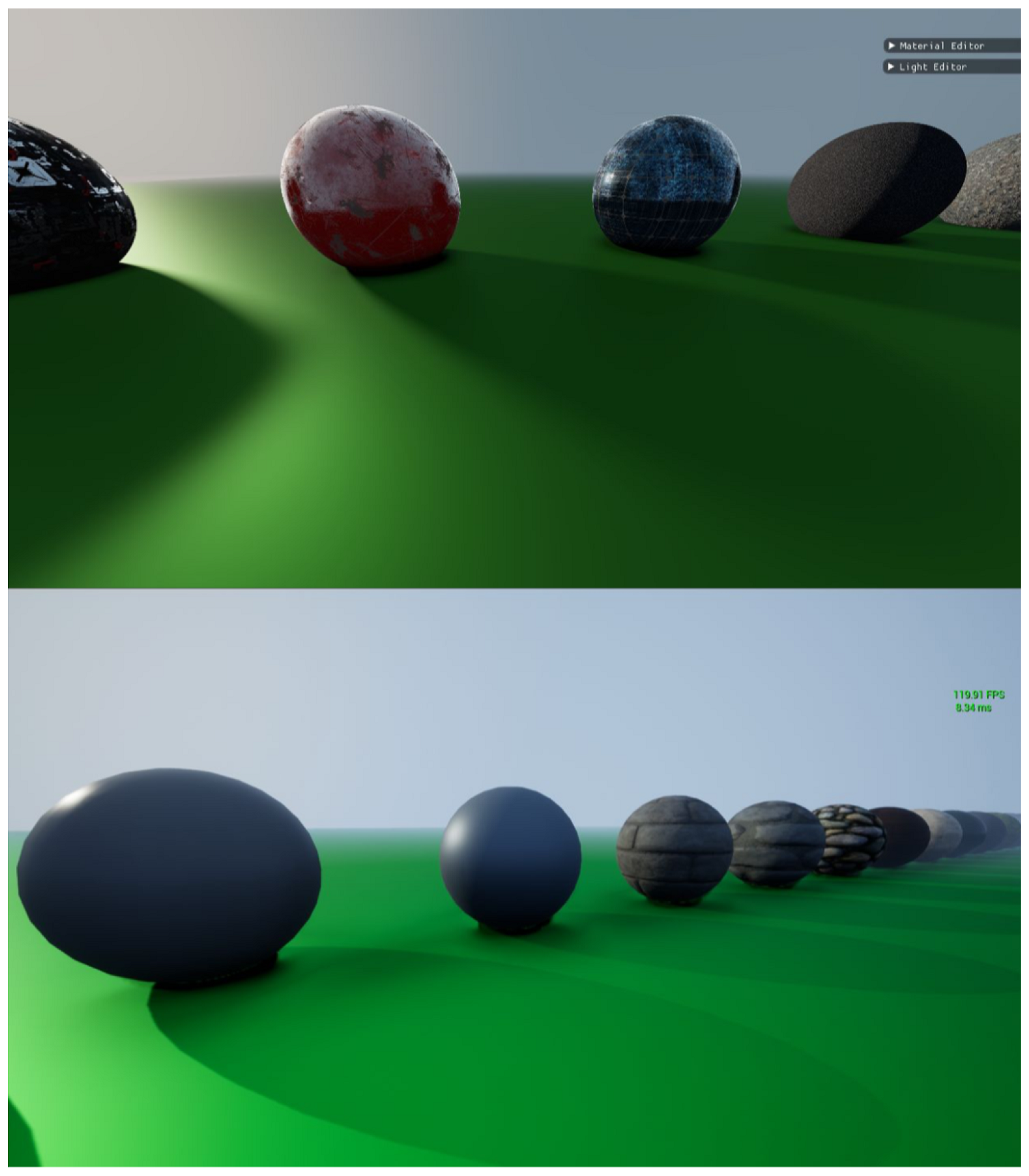
2.3. Material Format

A Material object holds information on how to shade a surface:

• albedo—the surface colour in linear, floating point RGB.
• metalness—a value in the range $[0\dots 1]$ corresponding to how ‘metalic’ a surface is in regard to specular and diffuse shading.
• roughness—a linear value from $[0\dots 1]$ corresponding to the smoothness of surface reflections and light scattering.
• $F_0$—the base reflectivity when metalness is set to zero in linear, floating point RGB. This often corresponds to a ’specular’ term in some PBR shaders (while others do not include this at all) and is included to allow for more complex material behaviours.
• triplar—a boolean value corresponding to XZ planar mapping (false) or triplanar mapping (true) for textures.
• normalStrength—a linear floating point value which scales normal deflection from normal map textures, useful when displacing a surface at a ’less steep’ angle than the normal map is designed for.
• albedoTex—the texture descriptor of the sRGB albedo map (or −1 when not used). The texture is multiplied by the albedo value.
• normalTex—the texture descriptor for the linear detail normal map (or −1 when not used).
• roughnessTex—the texture descriptor for the linear roughness map (or −1 when not used). The texture is multiplied by the roughness value.
• metalnessTex—the texture descriptor for the linear metalness map (or −1 when not used). The texture is multiplied by the metalness value.
• heightmapTex—the texture descriptor for the linear displacement heightmap (or −1 when not used). This texture is not used for shading but is instead used by an object SDF to add real geometric displacement.
• ambietTex—the texture descriptor for the linear ambient occlusion map (or −1 when not used).

The Material object has two constructors which are accessible from both host and device code. The first constructor takes albedo, metalness, roughness and $F_0$ values as arguments, assigning them as member-initialisers. The body of this constructor also sets all texture descriptors to −1 to specify the material as textureless by default, as well as setting the texture projection mode to planar and normal strength to 1. The second constructor, however, only takes albedo, roughness and metalness as parameters and calls the first constructor with these values as well as a default $F_0$ value of $[0.04,0.04,0.04]$ which is considered to be the ‘standard’ base reflectance for most non-metal dielectrics (i.e., plastics, organic materials).

2.4. Light Format

A Light object holds information on the lights present in a scene:

• position—a homogeneous 3D vector for the position of a light. When the 4th component is of value 1, the light represents a point light and a value of 0 represents a directional light with the first three components corresponding to the light direction. In the material editor, this is displayed as two separate values; a 3D position vector and a boolean value.
• colour—a homogeneous 3D vector for the colour of the light. The 4th component corresponds to the inverse of the light intensity. In the material editor, this is displayed as two separate values; a linear colour RGB value and a linear intensity value.
• attenuation—a 3 component vector corresponding to constant, linear and quadratic attenuation for the light. If a light is a sky light, the attenuation values are ignored and a value of [1,0,0] is used since the light is considered to be infinitely distant.
• hardness—a linear value corresponding to the ’softness’ of shadows cast by the light. A minimum value of 3 is considered maximum softness without artefacts and a maximum value of 128 is considered to cast perfectly sharp shadows.
• radius—a linear value corresponding to the maximum distance that a light can illuminate.
• shadowRadius—a linear value corresponding to the maximum distance that a light can cast shadows.
• shadows—a boolean value to enable (true) or disable (false) shadow casting.

Lights are stored in a vector on the host and copied once per frame to device memory in the same fashion as materials. The first two lights in the vector are special and are used to calculate the ‘sky’ and ‘fog’. The light editor can add and remove lights dynamically at run time.

2.5. Ray Format

Rays are objects used to represent a ray in device code. Information needed for the ray marching and lighting algorithms are stored inside the ray object:

• t—a floating point value representing the distance that the ray has currently marched to.
• h—a floating point value corresponding to the closest intersection distance from the most recent ray evaluation.
• marches—an integer for the current number of march iterations.
• evaluations—an integer for the current number of SDF evaluations.
• p—a 3D vector containing the current position of the ray in space.
• materialId—an integer corresponding to the material of the closest object.
• rayType—a bitfield enum value for the ray’s current purpose which can be any combination of the following:

  –

  camera (0x00001)—used for rays cast from the camera.

  –

  shadow (0x00010)—used for rays cast from a surface towards a light to calculate light occlusion or for rays used to calculate ambient occlusion.

  –

  reflection (0x00100)—used for singular rays that are cast for sharp specular reflections. (currently not used)

  –

  transmission (0x01000)—used for rays that compute transparent transmissions (camera | transmission) or subsurface scattering (camera|shadow). (currently not used)

  –

  normal (0x10000)—used for rays which calculate surface normals.

There are three device functions which are used by the ray marching algorithm:

• evaluate—a function that takes the SDF material identifier and distance sample and then returns the distance. This function increments the evaluation value and sets materialId and h if the distance is less than the previous value of h.
• isRay—a function that returns true if the ray is of the same type as the type argument.
• isOnlyRay—a function that returns true if and only if the ray is of the same type as the type argument only.

2.6. Surface Map

2.6.1. Signed Distance Function

A signed distance function in its simplest form takes a point in space and returns the signed distance from that point to the surface of that object. A library of primitive SDFs has been implemented for a wide range of implicit surfaces and for the purpose of the experiments in the present work; these are included in the accompanying code. Each SDF takes different parameters to reflect the different modifiable characteristics for each surface type (e.g., the orientation of a plane, radius of a sphere, angle of a cone, etc.). All SDFs do, however, share regular characteristics: the first parameter is always the position of the sample point in space, all return a bound for the distance field (although most are exact), and all implicit surfaces have the origin at $[0,0,0]$.

2.6.2. Map Function

In a ray marching algorithm, the purpose of the map function is to return the distance from a point in space to the closest surface, i.e., it can be said that the map function samples the minimum of all 3D distance fields. The distance field for a scene is defined as the overlapping minimum of all signed distance field functions evaluated at p. However, to enable more complex scenes, the map function used in this renderer takes different parameters:

• ray—a Ray object of the current ray being marched. This is required to update materials as well as to provide different functionality for the map function based on the type of ray.
• d_materialVector—the device material vector to allow for accessing heightmap textures to displace surfaces.
• offset—used by the normal calculation algorithm and ambient occlusion algorithm to scatter the points at which to sample the distance field without affecting the ray position itself.

2.7. Raymarching Algorithm

Raymarching is an iterative root-finding approximation of ray tracing given a field of geometric distances, see Figure 3. The process of building a frame comprises:

• Ray Generation Program—Generate camera rays given camera position, direction and focal length.
• March Calculation—March rays towards intersections given a map function.
• Normals Calculation—Compute normals and apply detailing.
• Surface Normal—Compute the surface normals from the distance field gradient given a map.
• Detail Normals—Use surface normals and material ID to deflect normals using a texture.
• Shade Intersection Pixel—Determine pixel colour using normals, materials and lights.
• Shading & Shadows—First shading pass using the Cook–Torrance BRDF (bidirectional reflectance distribution function), emitting only shadow rays towards lights and sampling the distance field for ambient occlusion.
• Specular Environment Shading—Compute specular reflections of the ‘skybox’, emitting only one shadow ray per camera ray, randomly distributed in a specular lobe.
• Diffuse Environment Shading—Compute diffuse lighting from the ‘skybox’, emitting only one shadow ray per camera ray, randomly distributed in a hemisphere oriented from the surface normal.
• Shade Sky & Fog—Determine colour of sky from camera ray direction and light colours and linearly interpolate between the shaded surface colour and sky colour based on intersection distance for fog.
• Tone Mapping—Map the unclamped linear color space into a clamped sRGB color space to approximate HDR (high dynamic range) imagery.
• Temporal AA—Use data from the previous frame to apply anti-aliasing.
• Write Pixel—Write computed pixel colours to the Pixel Buffer.

2.7.1. Ray Generation Program

The ray generation program is a function that computes ray origins and ray directions for camera rays. To build a frame of pixel width w and pixel height h, the kernel is launched with $w\times h$ threads, where each thread emits one initial camera ray. These threads are grouped into $8\times 8$ tiled blocks, consisting of two 32 thread wraps which are computed as SIMD (single instruction, multiple data) vectors. Given the ID of a thread within a block, and the ID of a block within the grid, it can be determined which pixel each thread corresponds to in 2D space, giving screen space coordinates. From these integer coordinates, floating point UV coordinates are computed, such that the top left pixel has coordinates $[-1,1]$ and the bottom right pixel has coordinates $[1,-1]$. Then, ray directions become:

$$\begin{array}{c}\hfill r{d}^0={\left[r{d}_x^{0}r{d}_y^{0}r{d}_z^0\right]}^T=\frac{{\left[uvf\right]}^T}{\sqrt{u^2+v^2+f^2}},\end{array}$$

(1)

where u, v, f are, respectively, the x coordinate of the UV, the y coordinate of the UV and the camera focal length, and $r{d}^0$ is a 3D direction vector. This process creates a ‘virtual matrix’ of vectors spanning across all threads representing a pinhole camera with focal length f oriented towards $[0,0,1]$. To orient the rays in the direction specified by the virtual camera, they must be transformed using two rotation matrices. Given the camera angles $\varphi$, $\theta$, the following transformation gives the correctly oriented ray direction $rd$:

$$rd=\left[\begin{array}{c}r{d}_x\\ r{d}_y\\ r{d}_z\end{array}\right]=\left[\begin{array}{ccc}cos\theta & 0& sin\theta \\ 0& 1& 0\\ -sin\theta & 0& cos\theta \end{array}\right]·\left[\begin{array}{ccc}1& 0& 0\\ 0& cos\varphi & -sin\varphi \\ 0& sin\varphi & cos\varphi \end{array}\right]\left[\begin{array}{c}r{d}_x^0\\ r{d}_y^0\\ r{d}_z^0\end{array}\right]$$

(2)

The only other vector needed to define a camera ray is $ro$ which is simply the 3D vector corresponding to the camera position. From this, any position p along this ray can be computed as $p=ro+rd·t$.

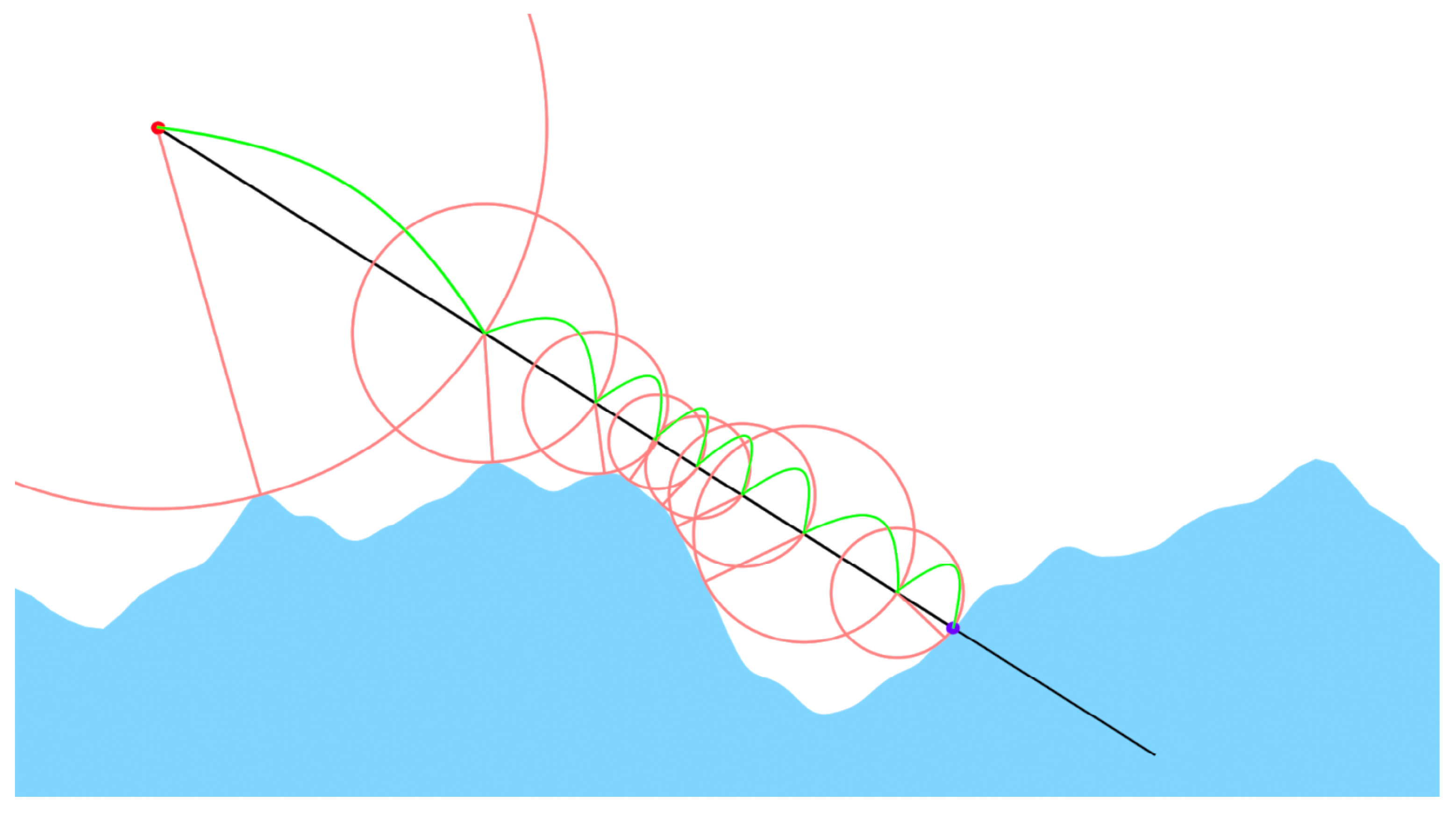
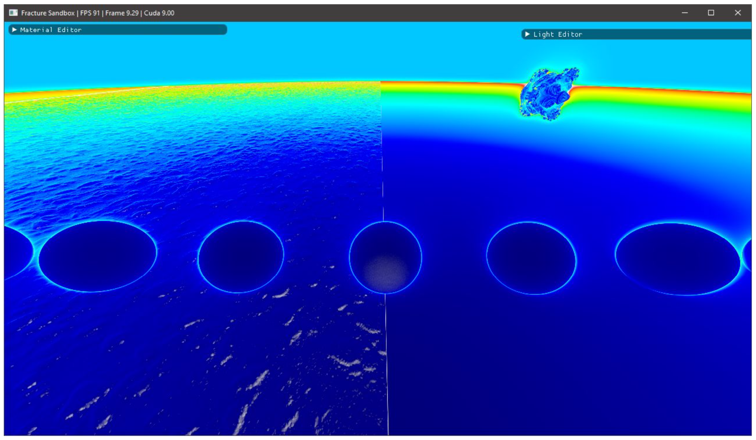
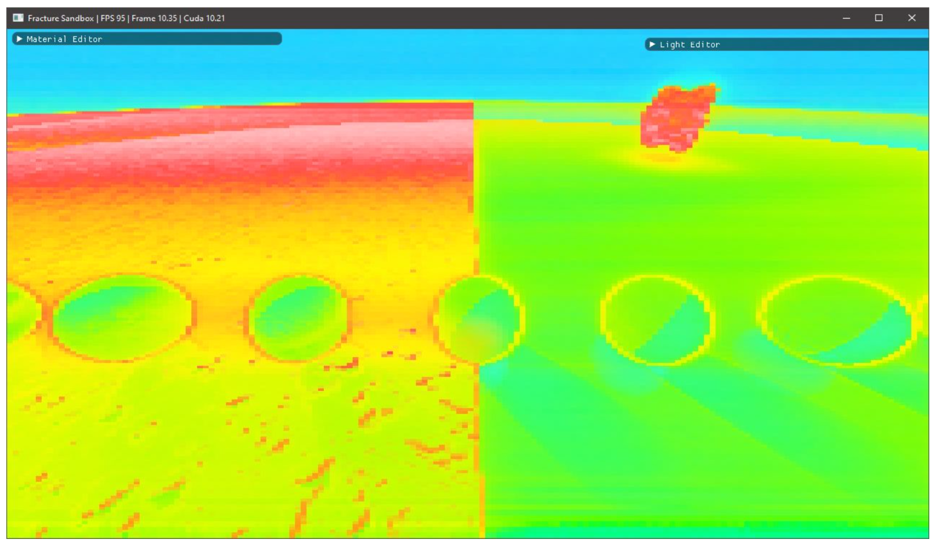
2.7.2. March Calculation

The first march calculation performed with camera rays is the determination of the intersections of each ray and the implicit surface union defined by the map function. In its simplest form, the march function can be defined using a recurrence relation with an intersection occurring at $ro+rd·t$ if $t=t_0,t_1,\dots ,t_n$ converges as $n\to \infty$ (otherwise, no intersection occurs):

$$\begin{array}{cc}\hfill march& =\underset{n\to \infty }{lim}{t}_n\hfill \end{array}$$

(3)

$$\begin{array}{cc}\hfill t_0& =t_{min}\hfill \end{array}$$

(4)

$$\begin{array}{cc}\hfill t_n& =t_{n-1}+h_{n-1}\hfill \end{array}$$

(5)

$$\begin{array}{cc}\hfill h_n& =map(ro+rd·t_n)\hfill \end{array}$$

(6)

where $t_{min}$ represents the near clipping plane. However, it is computationally impossible to iterate infinitely, so, instead, we impose a maximum iteration depth $n_{max}$ for n, a maximum $t_{max}$ limit for t (the far clipping plane), and a short circuit intersection distance $h_{min}$ for h. This results in a slightly different set of recurrence relations:

$$\begin{array}{cc}\hfill march& =t_{n_{max}}\hfill \end{array}$$

(7)

$$\begin{array}{cc}\hfill t_n& =\left\{\begin{array}{cc}{t}_{n-1},\hfill & \mathrm{if}{t}_{n-1}>t_{max}\hfill \\ t_{n-1}+h_{n-1},\hfill & \mathrm{otherwise}\hfill \end{array}\right.\hfill \end{array}$$

(8)

$$\begin{array}{cc}\hfill h_n& =\left\{\begin{array}{cc}0,\hfill & \mathrm{if}|h_{n-1}|<h_{min}\hfill \\ map(ro+rd·t_n),\hfill & \mathrm{otherwise}\hfill \end{array}\right.\hfill \end{array}$$

(9)

These formulae hold true for when all surfaces defined by $map$ have bounded or exact distance fields, but this is not true for all surface types; for example, a heightmap displaced plane will often give over estimations and underestimations for the distance field, which could potentially cause a ray to pass through high frequency displacements in the surfaces without detecting an intersection. To prevent this from happening, it is possible to change $h_n$ expression for the map case such that the result of the map function is multiple by a coefficient k where $0<k\le 1$. The smaller this coefficient is, the less likely an overestimation is to happen but with the cost of requiring more marches to reach an intersection than for a coefficient of exactly 1. The solution to this is to vary the value of k between neighbouring pixels and between consecutive frames and then use temporal anti-aliasing techniques to remove the resulting high frequency noise with Monte Carlo integration [9].

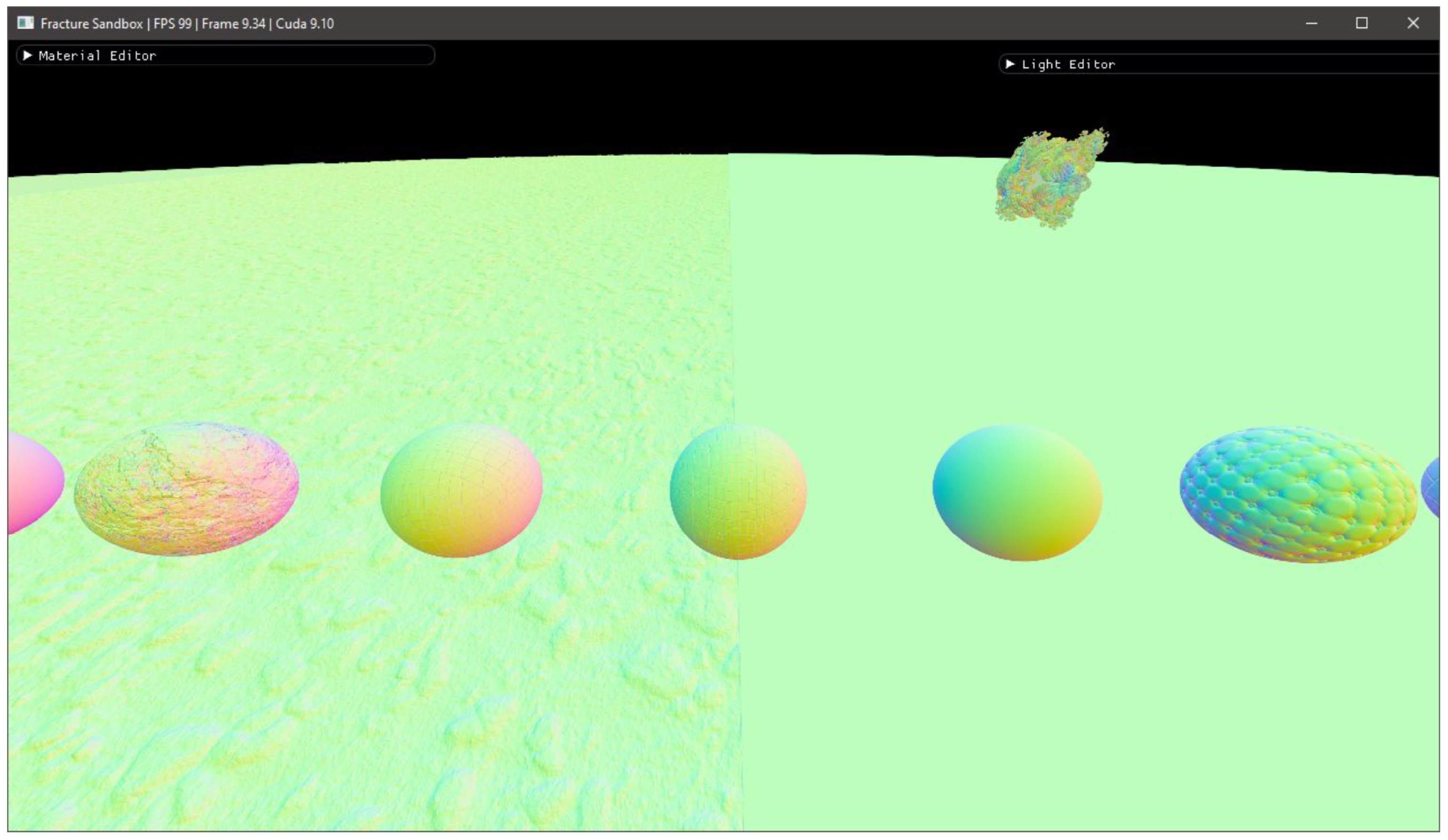
2.7.3. Normal Calculation

The normal of an implicit surface is defined via the three partial derivatives of the map function where the distance field is equal to zero (i.e., at an intersection point). At point p:

$$\begin{array}{c}\hfill normals\left(p\right)=\left[\frac{\partial }{\partial x}map\left(p\right),\frac{\partial }{\partial y}map\left(p\right),\frac{\partial }{\partial z}map\left(p\right)\right]=\nabla map\left(p\right)\end{array}$$

(10)

However, this requires that an analytical derivative for the map can be computed, which itself requires analytical derivatives for all SDFs. This is not necessarily possible as some surfaces may not have an analytical derivative or have an analytical derivative which would translate to performant device code.

Instead of obtaining the exact normal, it is possible to instead obtain an approximation, e.g., using forward differences or central differences. However, this results in a total of six map evaluations for the three partial derivatives, which could result in a lot of overhead for particular complex scenes. If we assume that $map\left(p\right)<<1$ due to p being at an intersection, it is possible to obtain the normal using only three evaluations of the map function when using the forward difference approach:

$$\begin{array}{c}\hfill normals\left(p\right)\approx normalize\left(\left[\begin{array}{c}map(p+h,0,0)\\ map(p+0,h,0)\\ map(p+0,0,h)\end{array}\right]\right)\end{array}$$

(11)

However, normals obtained in this way will be less numerically accurate. Instead, by using the Tetrahedron technique, it is possible to obtain surface normals with the same accuracy as the central difference approach using only four evaluations. This approach samples the distance field at four equidistant vertices of a tetrahedron giving four directional derivatives that can be summed together to give the approximation of the normal at the zero-isosurface:

$$\begin{array}{c}\hfill normals\left(p\right)\approx normalize\left(\sum _{i=0}^3{k}_{i}map(p+h{k}_i)\right)\end{array}$$

(12)

This technique is adopted in the proposed renderer for normal evaluation. One drawback (and of the previously discussed techniques) is that the normal value is inaccurate at sharp intersections of multiple surfaces. One way to avoid this would be to evaluate only the SDF of the closest object in place of the map. This can be achieved by altering the map function to take a ‘mask’ value such that only SDFs with the material ID obtained in the march step contribute to the distance field.

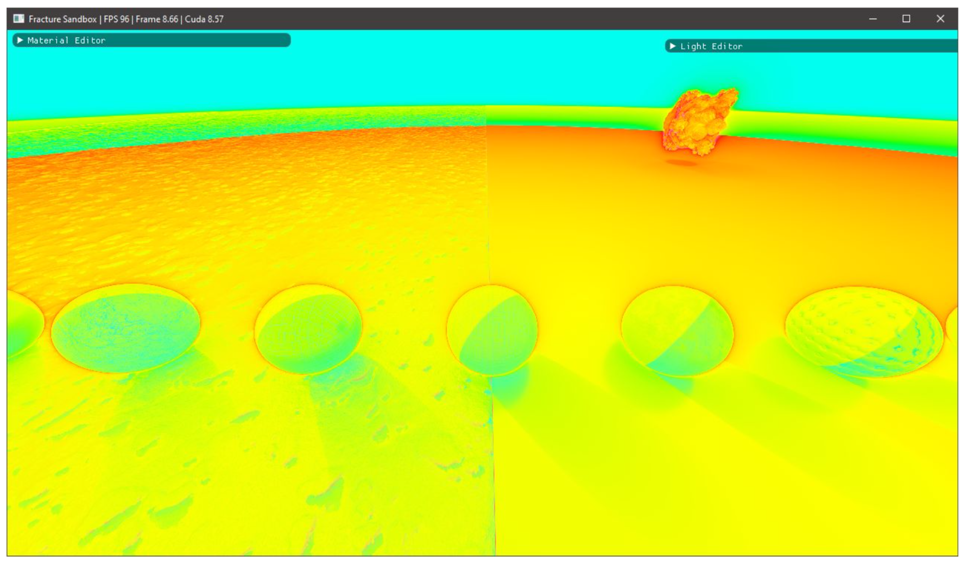
2.7.4. Ambient Occlusion

Ambient occlusion is the process of decreasing the luminosity of ambient light in the crease and crevices of geometry to simulate the effect occlusion of light based on object proximity. In a typical raster renderer, this is done using Screen Space Ambient Occlusion (SSAO) which uses the depth buffer and surface normals to approximate this effect. However, this can lead to unrealistic looking results. To improve the accuracy of AO in this renderer, the distance field itself is used to approximate occlusion; this process works by sampling equally spaced points perpendicular to the surface and calculating the weighted sum of deltas of surface distances with distance field distances to approximate how occluded that surface is from surrounding geometry.

2.7.5. Shadow Occlusion

In computer graphics, light sources are often modelled as point sources. Hence, shadows cast by the light are always sharp, as a point on a surface is either fully occluded by other geometry (in shade) or not at all (fully lit). This differs from reality where light sources have a spatial extent, and a point in space can be partially occluded. This results in soft shadows with penumbra. In a raster engine, this can be achieved by applying a distance based low pass filter to the shadow map which must be recomputed every frame to allow for dynamic geometry and lighting. However, in a raymarching based renderer, it is possible to use the distance field to approximate soft shadows.

To cast hard shadows from a light in a raymarching engine, the following algorithm is used:

• Determine point p on the zero-isosurface of the distance field.
• Cast a shadow ray at point p and raymarch to light position $p_l$, determining the intersection t.
• If $t<|p-p_l|$ point p is fully occluded, otherwise the point is fully lit.

With a simple modification, it is possible to transform the hard shadow algorithm into one that supports soft shadows without any extra performance cost; instead of only tracking t to determine occlusion, the algorithm also tracks the minimum penumbra factor $re{s}_n$ at each raymarch iteration. The penumbra factor is calculated as:

$$\begin{array}{c}\hfill re{s}_n=min\left(re{s}_{n-1},\frac{kh}{t}\right),\end{array}$$

(13)

where $re{s}_0$ is initialised with a value of 1 (no occlusion), k is a coefficient for the shadow hardness, and h, t are the surface distance and ray position coefficient as defined in the raymarching recurrence relations. Hence, the recurrence relations for the soft shadow casting algorithm become:

$$\begin{array}{cc}\hfill SoftMarch& =re{s}_{n_{max}}\hfill \end{array}$$

(14)

$$\begin{array}{cc}\hfill {res}_0& =1\hfill \end{array}$$

(15)

$${res}_n=\min \left(re{s}_{n-1},\frac{k{h}_{n-1}}{t_{n-1}}\right).$$

(16)

2.8. Lighting Model

Once the ray surface intersection has been determined, along with the surface material, surface normals and detail normals for all data needed to shade a pixel have been obtained. Our renderer uses a Physically Based Rendering (PBR) lighting model based on the Cook–Torrance BRDF [10] which more accurately represents the real world than Phong’s model [11].

2.8.1. Cook–Torrance Based BRDF

For a lighting model to be considered PBR, it must:

• use the microfacet surface model,
• conserve energy when reflecting light, and
• use a physically based BRDF such as Cook–Torrance.

The microfacet surface model is a statistical approximation for a surface’s roughness given a roughness parameter. The sharpness of specular reflections of a surface is proportional to the probability of the halfway vector h being aligned with microfacet normals $n_f$ where the halfway vector is defined as [12]:

$$\begin{array}{c}\hfill h=\frac{l+v}{\parallel l+v\parallel }\end{array}$$

(17)

where l, v are the incoming light and view vectors, respectively. This model also, conveniently, ensures energy conservation such that the energy of outgoing light from a surface cannot exceed the energy of incoming light. Phong’s model [11], probably the most common reflectance model used, fails in this respect and thus produces obviously unrealistic shading. To ensure the conservation of energy, the diffuse shading component $k_d$ should be multiplied by $1-k_s$, where $k_s$ is the specular counterpart [10].

The reflectance equation describes the outgoing light $L_o$ as the sum of emitted light $L_e$ and reflected light. Reflected light is the sum of all incoming light $L_i$ multiplied by the surface reflection $f_r$ (the BRDF) and the cosine of the incident angle. This leads to the following expression:

$$\begin{array}{c}\hfill L_o=L_e+{\int }_{\Omega }\left(f_r{L}_i\right)\left({\omega }_i·n\right)d{\omega }_i,\end{array}$$

(18)

where $\Omega$ is the unit hemisphere aligned with surface normal n [13]. For the surface reflectance function $f_r$, herein we adopted the Cook–Torrance BRDF [10], which is the weighted sum of the Lambertian diffuse and Cook–Torrance specular terms:

$$\begin{array}{c}\hfill f_r=k_d{f}_{Lambert}+k_s{f}_{CookTorrance}\end{array}$$

(19)

where $k_d$ and $k_s$ are the weightings of the diffuse and specular terms, respectively, and $k_d+k_s=1$ so as to ensure the conservation of energy. The Lambertian diffuse term is simply described as the surface albedo c normalized for integration over the hemisphere. This gives the the Lambertian term:

$$\begin{array}{c}\hfill f_{CookTorrance}=\frac{c}{\pi }\end{array}$$

(20)

The Cook–Torrance specular term is more complex. It is defined as the product of three functions D,F,G divided by fourfold the product of the dot product between the surface normal n and the outgoing light direction ${\omega }_o$ with the dot product of the surface normal and the negative of the incoming light direction ${\omega }_i$:

$$\begin{array}{c}\hfill f_{CookTorrance}=\frac{DFG}{4\left({\omega }_o·n\right)\left({\omega }_i·n\right)}\end{array}$$

(21)

The three functions are used to approximate different parts of a surface’s reflective properties. D, the normal distribution function, approximates the probability of surface microfacets being aligned with the halfway vector based on the surface roughness. G, the geometry function, describes the self-shadowing property of microfacets, where rough surfaces may have some microfacets that occlude light reflections caused by other microfacets. F, the Fresnel equation, describes the ratio of surface reflections at different surface angles.

For the normal distribution function, the Trowbridge–Reitz GGX approximation is used [14,15]. Given the surface normal n, halfway vector h and roughness parameter $\alpha$:

$$\begin{array}{c}\hfill D_{GGXTR}(n,h,\alpha )=\frac{{\alpha }^2}{\pi {\left({\left(n·h\right)}^2\left({\alpha }^2-1\right)+1\right)}^2}\end{array}$$

(22)

At low roughness, there is a highly concentrated number of microfacets that are aligned with the halfway vector, causing a bright specular highlight in a small radius. At high roughness, it is more likely to find microfacets aligned with the halfway vector over a larger radius, causing the size of the specular highlight to decrease with increasing roughness while the highlight intensity decreases.

The Geometry function uses the Schlick-GGX function [16] to calculate the self shadowing probability along a particular vector based on roughness, as well as using Smith’s method to compute the incoming and outgoing light self shadowing probabilities. Given surface normal n, view vector v, light vector l and roughness $\alpha$, the following formulas are used to compute the geometry function G:

$$\begin{array}{cc}\hfill G(n,v,l,\alpha )& =G_{Schlick}(n,v,k)G_{Schlick}(n,l,k)\hfill \end{array}$$

(23)

$$\begin{array}{cc}\hfill G_{Schlick}(n,i,k)& =\frac{n·i}{(n·i)(1-k)+k}\hfill \end{array}$$

(24)

$$\begin{array}{cc}\hfill k& =\frac{{(\alpha +1)}^2}{8}\hfill \end{array}$$

(25)

The Fresnel equation describes the ratio of light reflected over light that gets refracted which is dependent on the relative viewing angle of the surface. A surface has a base reflectivity given by $F_0$ which determines the reflectivity of the surface when the view and normal vectors are aligned; this value is based off the wavelength-dependent indices of refraction, but our approximation only uses base reflectance values for the red, green and blue wavelengths. The base reflectance value is precomputed and is often near zero for non-metals and near one for metals (being somewhere in between for semiconductors).

The equation used is the Fresnel–Schlick approximation [17], which models specularity as having a fifth power weighting at grazing angles (a commonly used approximation for specularity):

$$\begin{array}{c}\hfill F(h,v,F_0)=F_0+(1-F_0){(1-h·v)}^5\end{array}$$

(26)

The value $F_0=0.04$ is the default for materials in this engine for non-metals, and is equal to the albedo for metallic surfaces (i.e., when the metalness parameter is equal to 1). However, custom values may be used as described in Section 2.3. The Fresnel equation is also used for the diffuse coefficient component, where $k_d=1-F$.

Combining all the above formulae:

$$\begin{array}{c}\hfill L_o={\int }_{\Omega }\left((1-F)\frac{c}{\pi }+\frac{DFG}{4\left({\omega }_o·n\right)\left({\omega }_i·n\right)}\right)(L_i{\omega }_i·n)d{\omega }_i\end{array}$$

(27)

Light radiance $L_i$ is calculated with the light colour $l_{dehomogenized}$, the polynomial attenuation model coefficients $A_{Constant}$, $A_{Linear}$, and $A_{Quadratic}$, distance d, and light radius r, which leads to:

$$\begin{array}{cc}\hfill L_i& =\left(\frac{l_{dehomogenized}}{A_{Constant}+d{A}_{Linear}+d^2{A}_{Quadratic}}\right)\left(\frac{r-d}{r}\right)\hfill \end{array}$$

(28)

$$\begin{array}{cc}\hfill l_{dehomogenized}& =\left[\frac{l_r}{l_w},\frac{l_g}{l_w},\frac{l_b}{l_w}\right]\hfill \end{array}$$

(29)

where ${\left[l_r,l_g,l_b,l_w\right]}^T$ is the homogeneous light colour vector. The second term in the radiance equation is responsible for interpolating the light radiance down to zero as the distance coefficient approaches the light radius. This allows for a smooth transition to zero radiance as the distance of the surface to the light reaches the radius, allowing for the light to be skipped when beyond the maximum radius.

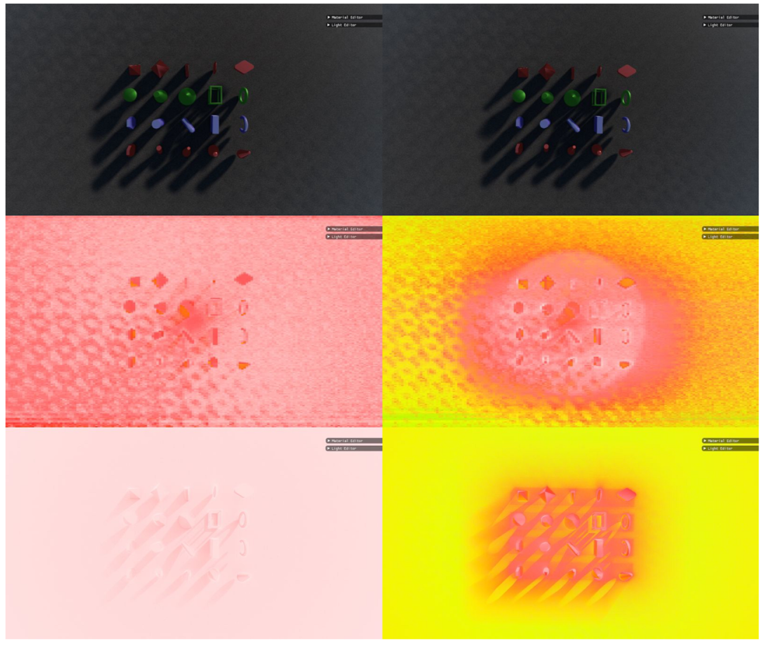
2.8.2. Texture Mapping

Texture mapping is the process of wrapping a 3D surface in a 2D texture. In a typical raster engine, this is done by assigning UV coordinates to the vertices of a mesh; the UV coordinates correspond to the $x,y$ coordinates of the texture being used. These values are then interpolated between per fragment and are used to sample the texture. This approach, however, is not suitable for procedural rendering since there are no meshes being used. Instead, we must use projection techniques to map a texture to an arbitrary point in space based on procedural surface information.

Planar projection mapping is one such technique. This takes two of the three coordinates of a point on the zero-isosurface and uses them to sample the 2D texture. The default axis for planar projection mapping in this raymarching engine is the $xz$-axis, since this is the same axis as the ‘floor plane’. To obtain the texture colour for position p in space and texture sampling function $sample(u,v)$, the following formula is used for planar projection texture mapping:

$$\begin{array}{c}\hfill textur{e}_{planar}\left(p\right)=sample(p_x,p_z)\end{array}$$

(30)

Planar projection is suitable for planar surfaces, such as floors, walls, ceilings, etc, but it is unsuitable for more complex surfaces such as spheres as this will cause the textures to stretch as the angle between the surface normal and the normal of the projection plane increases. A solution to this is to apply planar mapping in three perpendicular planes and apply interpolation based on the surface normal alignment. This is called triplanar mapping, also known as round cube mapping. To do this, we require both the position p and surface normal n. This gives a simple formula with three texture lookups weighted by the absolute normal contribution for that axis.

$$\begin{array}{c}\hfill textur{e}_{triplanar}(p,n)=\frac{|n_x|sample(p_y,p_z)+|n_y|sample(p_x,p_z)+\left|n_z\right|sample(p_x,p_y)}{|n_x|+|n_y|+|n_z|}\end{array}$$

(31)

This function can be further parameterized with a ‘hardness’ parameter k which allows for the contribution of each planar texture sample to be weighted more or less heavily based on alignment. By taking the $k$th power of the absolute normal, the following formula for weighted triplanar mapping emerges:

$$\begin{array}{c}\hfill textur{e}_{triplanar}(p,n,k)=\frac{|n_x{|}^{k}sample(p_y,p_z)+|n_y{|}^{k}sample(p_x,p_z)+{\left|n_z\right|}^{k}sample(p_x,p_y)}{|n_x{|}^k+|n_y{|}^k+{\left|n_z\right|}^k}\end{array}$$

(32)

Triplanar mapping is suitable for shading since it results in a maximum of three samples per texture per camera ray. However, it is not suitable for the sampling of heightmaps in the $map$ function, as the texture lookups happen each iteration during marching, which results in a much larger memory bandwidth overhead than simple biplanar mapping which uses only one texture lookup.

2.8.3. Global Illumination

Global Illumination (GI) is the process of modelling light bounces to allow for indirect lighting illumination. GI improves the realism of a scene (in comparison to uniform ambient lighting across a scene) at the cost of additional processing.

The GI solution that was implemented for this renderer only takes into account the lighting contribution of the ‘sky’ with only a single bounce towards the sky hemisphere. In typical raster based renderers, the sky itself does not contribute to the illumination of surfaces but instead is modelled as one or more directional lights used to cast light (normally a ‘sun’ light casting a strong yellow-white light and a vertical directional ‘sky’ light casting a weaker bluish tone), e.g., as in Source Engine. This solution, however, results in inaccurate shadowing and can result in a much darker scene. The solution we propose comprises the creation of a virtual skybox of infinite directional lights casting inwards towards the scene and then sampling the skybox over a hemisphere directed away from the surface normal to contribute the diffuse contribution of the sky.

To sample the skybox in this way, we must cast shadow rays uniformly distributed over the normal hemisphere and calculate the radiance using Lambertian diffuse shading scaled by the soft shadow contribution. The radiance for diffuse GI from the sky is computed as:

$$\begin{array}{c}\hfill G{I}_{diffuse}=k_d\frac{c}{\pi }{\int }_{\Omega }sky\left({\omega }_i\right)SoftMarch(p,{\omega }_i,3)n·{\omega }_{i}d{\omega }_i\end{array}$$

(33)

with a shadow hardness of $k=3$ used to simulate the wide radius over which the sky is being sampled.

Since numerically integrating fully over the hemisphere is computationally impossible, we must instead sample the hemisphere uniformly. Given two random temporal samples $tempora{l}_x$, $tempora{l}_y$, and the surface normal n, a random sample direction ${\omega }_i$ is obtained as follows:

$$\begin{array}{cc}\hfill {\omega }_i& =sampl{e}_{hemi}(tempora{l}_x,tempora{l}_y,n)=\{T,B,N\}·H\hfill \end{array}$$

(34)

$$\begin{array}{cc}\hfill H& =\left\{cos\varphi sin\theta ,sin\varphi sin\theta ,cos\theta \right\}\hfill \end{array}$$

(35)

$$\begin{array}{cc}\hfill T& =\left\{\begin{array}{cc}\{0,0,1\}\times N,\hfill & if|n_z|<0.999\hfill \\ \{1,0,0\}\times N,\hfill & \mathrm{otherwise}\hfill \end{array}\right.\hfill \end{array}$$

(36)

$$\begin{array}{cc}\hfill B& =N\times T\hfill \end{array}$$

(37)

$$\begin{array}{cc}\hfill \varphi & =2\pi tempora{l}_x\hfill \end{array}$$

(38)

$$\begin{array}{cc}\hfill \theta & =0.5\pi tempora{l}_y\hfill \end{array}$$

(39)

The more samples taken per frame, the more accurate the lighting is at the cost of increased computation. By taking only one sample per frame, the image has a distinct checkerboard pattern when temporal AA is disabled, but when temporal AA is enabled, an accurate image is produced within only a few frames owing to the effective Monte Carlo integration over the hemisphere over time. The diffuse GI calculated here is added to the pixel colour of the first shading pass.

2.8.4. Reflections

Real-time reflections are difficult to accurately produce for any rendering method, often resulting in needing screen space techniques to approximate the reflections. The approach we take is to sample the skybox in a similar fashion as with the GI algorithm; by using the Cook–Torrance specular term (instead of the Lambertian diffuse term) and and by sampling the skybox with a specular lobe distribution (instead of a uniform uni hemisphere).

We can construct an equation for the specular global illumination in a similar way to the diffuse equation using the specular term of the Cook–Torrance BRDF and a shadow hardness based on the surface roughness $\alpha$:

$$\begin{array}{c}\hfill G{I}_{specular}=k_s{\int }_{\Omega }\left(\frac{DFG}{4\left({\omega }_o·n\right)\left({\omega }_i·n\right)}\right)sky\left({\omega }_i\right)SoftMarch\left(p,w_i,3+\frac{1}{\alpha }\right)n·{\omega }_{i}d{\omega }_i\end{array}$$

(40)

To sample the hemisphere in a biased specular lobe, a different sample function is required. GGX Importance Sampling can be summarized by the following equation (note that the sample function is almost identical to the hemisphere function with the addition of the roughness parameter $\alpha$):

$$\begin{array}{cc}\hfill {\omega }_i& =sampl{e}_{GGX}(tempora{l}_x,tempora{l}_y,n,\alpha )=\left\{T,B,N\right\}·H\hfill \end{array}$$

(41)

$$N=n$$

(42)

$$\begin{array}{cc}\hfill cos\theta & =\sqrt{\frac{1-tempora{l}_x}{1+({\alpha }^2-1)tempora{l}_y}}\hfill \end{array}$$

(43)

Like the diffuse GI, the specular reflections rely on temporal anti-aliasing for an accurate result with Monte Carlo integration over time. The specular GI calculated here is added to the pixel colour computed from the first shading pass and diffuse GI pass.

3. Evaluation

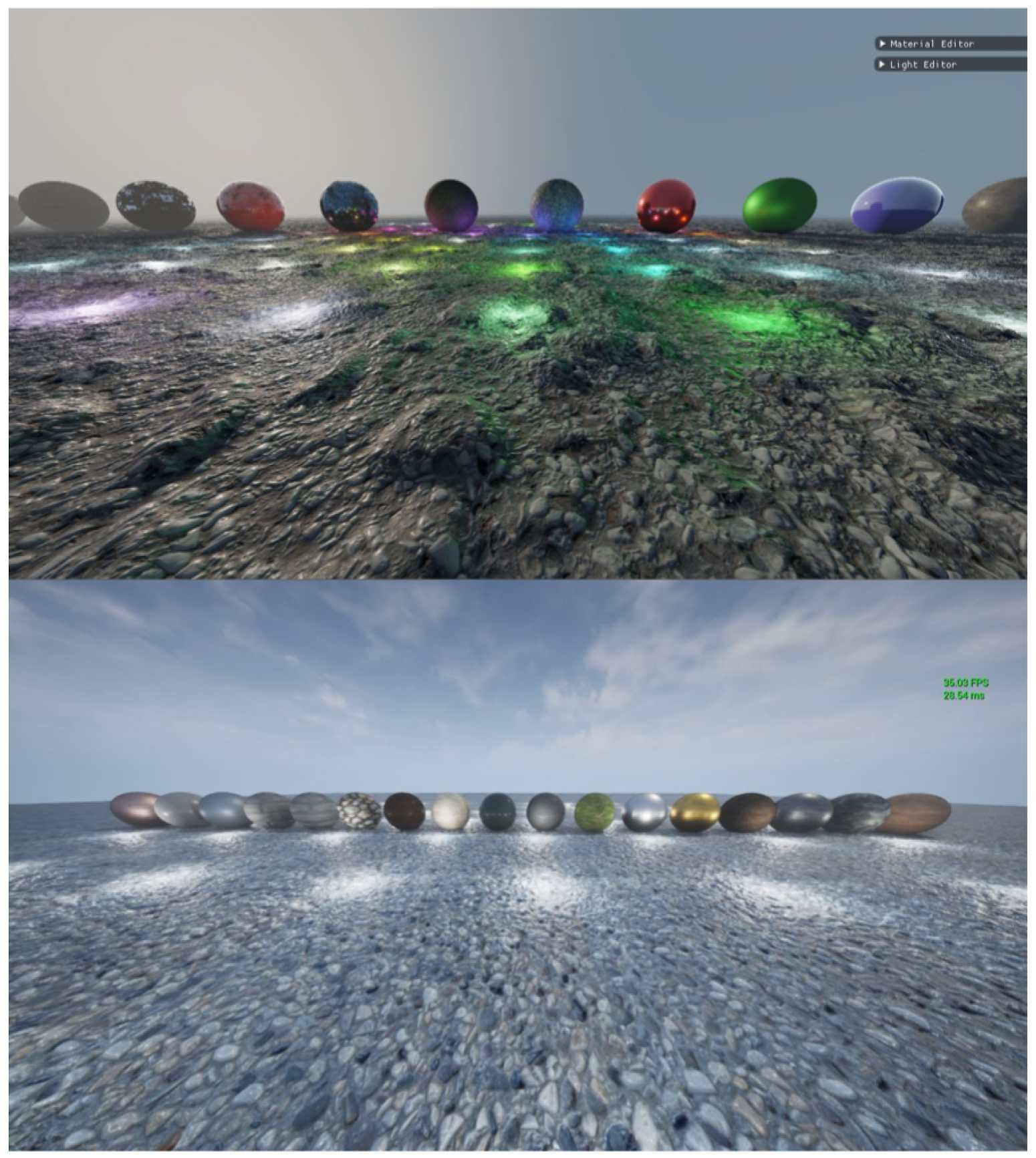
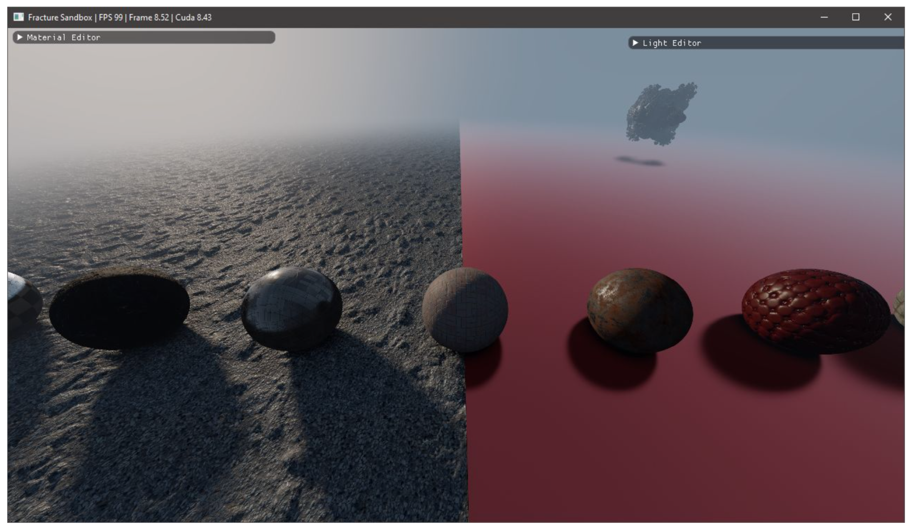
3.1. Visual Fidelity

The real-time visual fidelity achieved by this renderer is comparable to offline high fidelity techniques such as ray tracing, as well as surpassing techniques used by real-time raster renderers in both performance and quality. All images in this section were rendered at 1280 × 720 on an RTX 2080 Super. All comparisons were made against Blender engine version 2.90 and UE4 version 4.25.3.

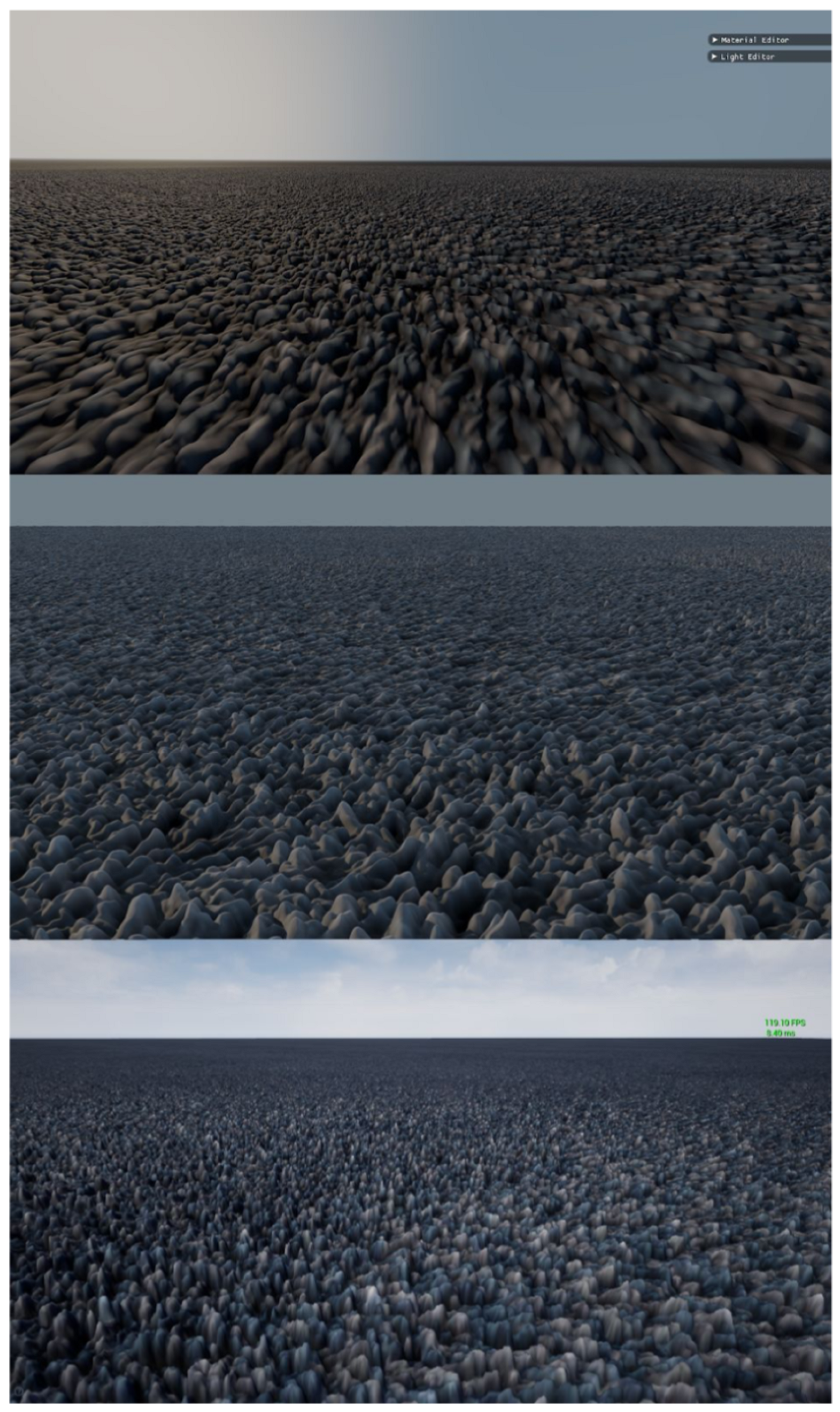
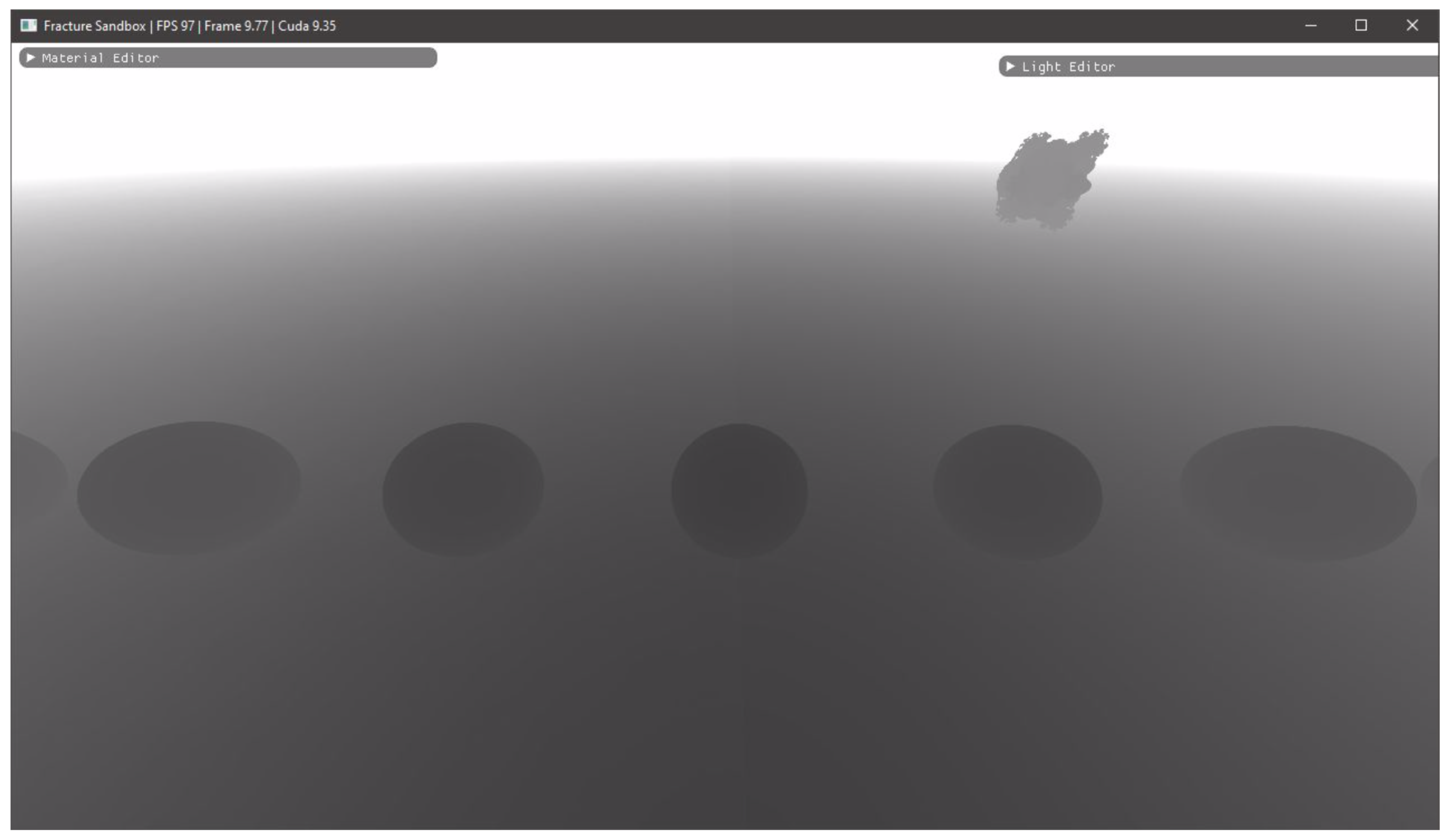
3.1.1. Displacements

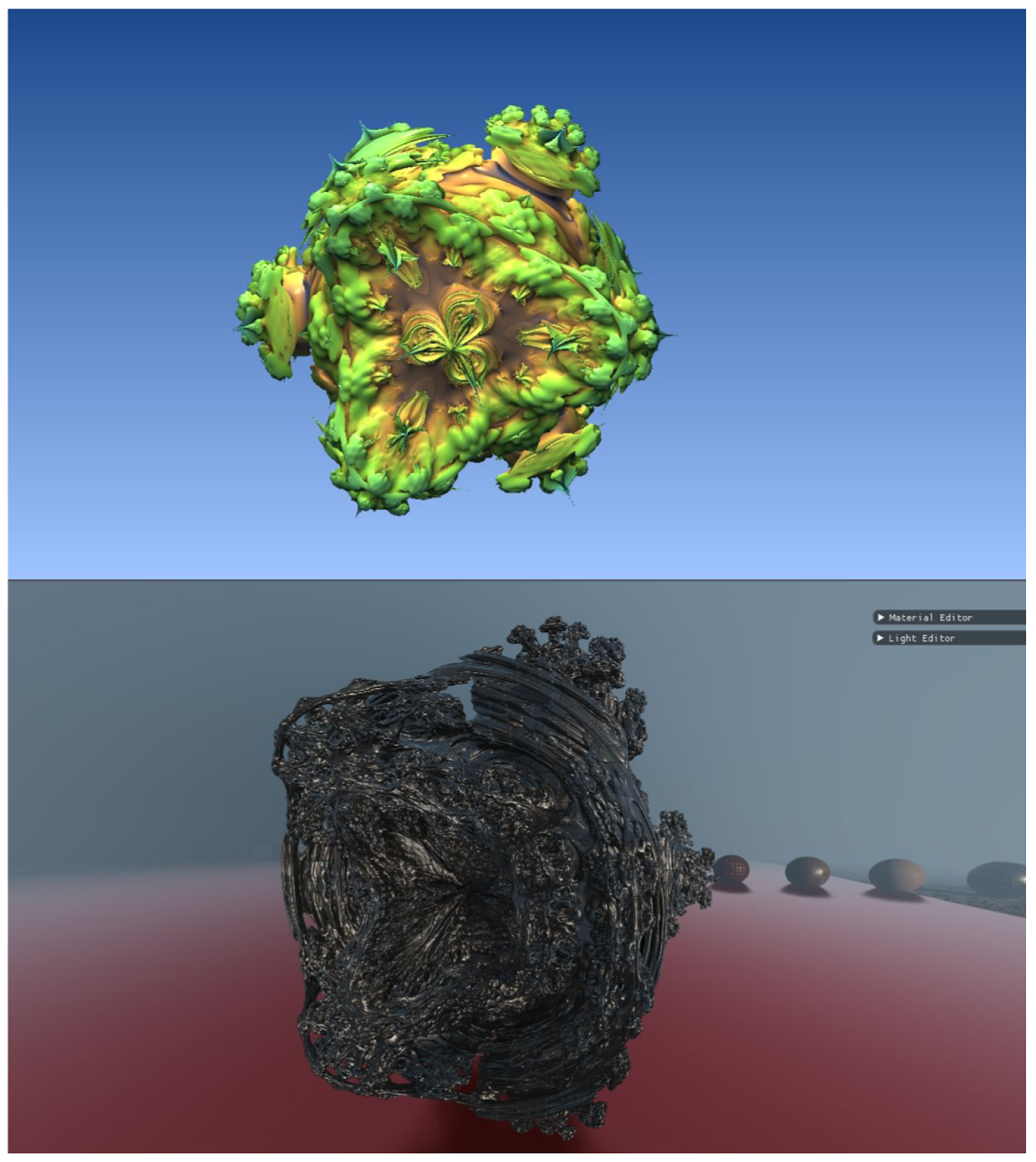
An insightful testing example is that of displaced planes rendering at very high framerates. There are three techniques for displaying detailed surfaces with microdisplacements: geometry displacement, parallax occlusion mapping and raymarching. We recreated a scene from the demonstration scene in Blender and UE4 for the purposes of comparison, see Figure 4.

The raymarched render of the carpet is produced with a frame duration of less than 8 ms and a video memory footprint of 1 GB (although this is mostly due to storing the textures needed for the full demo even though only the carpet is visible). Owing to TAA, the produced image is fairly photorealistic with fine detail. The main advantage of this method is the high image fidelity without computing any actual geometry while still supporting global shadowing and self shadowing. The primary disadvantage of this technique is requiring expensive texture lookups on each iteration.

The image produced by ray tracing with Cycles is also photorealistic with outstanding detail, although it took a whole 9 s with Nvidia OptiX acceleration to render with a peak video memory footprint of 3 GB, which was mostly due to needing to store the data for all vertices, which is the main disadvantage of this technique. Despite this, the image produced is remarkably accurate, including the multibounce shadowing interactions within the crevices of the carpet. The image produced with parallax occlusion mapping in UE4 is also as photorealistic and as performant as the raymarched image, taking under 9 ms to produce the image with a video memory footprint of 400 MB. Like raymarching, no actual geometry is computed, making it very lightweight. However, this technique comes with significant disadvantages such as being unable to produce dynamic self shadows and being unable to cast global shadows onto other objects of the scene. Another drawback is the visible ‘stair-stepping’ of the surface when viewed up close and at sheer angles, where the effect breaks down completely. This system also requires expensive texture lookups like the raymarching solution.

From this example, it is clearly evident that raymarching is on par with parallax occlusion mapping with regard to resource usage and is arguably of a better quality with no visible artefacts when Temporal Anti-Aliasing is enabled for the raymarcher.

3.1.2. Fractals

Another revealing test case is the rendering of fractals, see Figure 5. The main free renderer used for fractals is Mandelbulb3D (MB3D), a very cumbersome to use program which only supports CPU based rendering and had remained, up until 2015, when it was taken over by a new maintainer, closed source. Since the program takes no advantage of hardware acceleration, it often takes several seconds to produce an image.

MB3D lacks many features present in our renderer, such as texture support, support for other implicit surface types, HDR lighting, PBR shading, etc. MB3D works using a similar technique called fixed step ray marching, where a binary search is performed with fixed sample positions along a ray to determine the intersection surface.

Overall, MB3D is a poor candidate for the real-time rendering of fractals when compared to our raymarching renderer that is able to render fractals in real time in under 10 ms per frame in addition to supporting reflections, shadows, texturing and anti-aliasing.

3.2. Lighting

Shadow casting is an important feature of a realistic renderer. Regardless of the technique used, it is costly to compute. We recreated a scene which includes multiple spheres with different materials and 64 point lights all casting shadows to compare the performance of our raymarcher and a commercially available engine, see Figure 6 and Figure 7.

Both engines run at about 30 frames per second, giving comparable performance; however, in UE4, the point lights are unable to cast shadows correctly on the floor plane due to the drawbacks of parallax occlusion mapping. Both renderers produce similarly realistic lights with specular reflections as well as shadow reflections which are both achieved through temporal anti-aliasing. When the point light shadows are disabled, both engines run at much higher frame rates at an upwards of 90+ frames per second.

Another important part of rendering realistic lighting is the ability to cast soft shadows. We recreated another scene from the demo in UE4 and tried to match the lighting conditions as close as possible.

It is clear to see that UE4 struggles to cast soft shadows in such a simple scene due to the nature of rasterized shadow maps not taking into account shadow penumbras. Another interesting phenomenon to note is that the sphere geometry is visible in UE4 in the shadows due to meshes being comprised of triangles as opposed to raymarching where surfaces have exact mathematical representations.

It should also be noted that UE4 is running with frame durations of around 8 ms while our raymarching renderer runs with around 6 ms frame durations, meaning the Monte Carlo integration via TAA converges on realistic light conditions 20% faster in the proposed renderer than UE4 for this scene.

3.3. Bounding Volume Optimisation

A scene may be filled with dozens or even hundreds of surfaces that all add significant computation cost to the map function which may be evaluated at many millions of times per frame. To help improve the performance of the renderer, it is important to minimise the cost of the map function by ’skipping’ the evaluation of SDFs for objects that do not contribute to minimal distance field. Optimisation through bounding volumes is one such method which is explored in this work. The most performance intensive part of the demo scene is an array of 20 primitives which are all fairly expensive to evaluate, see Figure 8.

When BV optimisation is enabled, the renderer runs with an average frame duration of 21 ms (48 frames per second) and 41 ms when disabled (24 frames per second) at 720p. The clock cycle view clearly shows that the computation cost is relatively uniform across the entire frame when optimisation is disabled; however, with bounding volume optimisation enabled, the expensive computations are localised to areas of the frame where the complex geometry is present.

A similar phenomenon can be observed in the SDF evaluation views where the outlines of the bounding volumes are visible around the rows of primitives when enabled. It is also evident that fewer evaluations occur in areas of shadow due to a decreased number of map evaluations upon shadow rays converging on the casting surface.

Although a GPU is often considered SIMD, it is actually more accurate to describe modern GPUs as MIMD since different Streaming Multiprocessors (SMs) can process different instruction streams simultaneously over one or more thread warps per SM. Combined with the fact that the GPU is saturated with threads for this workload (i.e., more threads are scheduled than slots available to simultaneously compute them), the GPU can finish computation of the cheaper parts of the frame early and distribute the more expensive threads across the available SMs.

Lastly, as a means of providing additional insight into the performance of our engine, using an example scene shown in Figure 9, in Figure 10, Figure 11, Figure 12, Figure 13 and Figure 14, we provide a series of renderings, some of which illustrate the results of different intermediate computational stages of a rending and others which quantify in an easily comprehensible manner the associated computational burden.

4. Conclusions and Future Work

In this paper, we introduced what is to the best of our knowledge the first framework for real-time 3D rendering of complex scenes in CUDA using raymarching. We developed and described comprehensively a carefully engineered raymarching render engine, and demonstrated its effectiveness and superiority over popular alternatives using a series of empirical experiments. The performance and visual fidelity of the renderer is able to match and surpass that of free and commercial software solutions, proving major promise in the future of computer graphics. In addition, each element of the engine was discussed in detail, with observation insights that should assist in future research on production grade rendering pipelines. Lastly, we accompany our contribution with the full source code of a working prototype (the code can be accessed via the following URL: https://oa7.host.cs.st-andrews.ac.uk/raymarching_code.zip accessed on 1 November 2021).

Our development opens multiple avenues for future work. One direction we would like to explore involves experimenting with different pipelines for the raymarcher, e.g., experimenting with a draw call system like that used in OpenGL to draw objects into a depth buffer with multiple separate smaller maps. This could effectively result in a ‘deferred raymarcher’ which could result in the support of mixed-mode rendering to integrate rasterization of meshes into the pipeline.

Another direction for future work involves experimenting with the use of shadow maps for lights and ambient light capture probes for global illumination which could be computed at a different frequency from the primary view (i.e., at a low frame rate) to allow for high frame rate computation of the world with lighting that updates at a slightly slower rate.

References

1. Hart, J.C.; Sandin, D.J.; Kauffman, L.H. Ray tracing deterministic 3D fractals. In Proceedings of the 16th Annual Conference on Computer Graphics and Interactive Techniques, Boston, MA, USA, 31 July–4 August 1989; pp. 289–296. [Google Scholar]
2. Hart, J.C. Sphere tracing: A geometric method for the antialiased ray tracing of implicit surfaces. Vis. Comput. 1996, 12, 527–545. [Google Scholar] [CrossRef]
3. Quilez, I. Rendering Worlds with Two Triangles with Ray Tracing on the GPU. 2008. Available online: https://www.iquilezles.org/www/material/nvscene2008/rwwtt.pdf (accessed on 10 June 2021).
4. Quilez, I. Making a Simple Apple with Maths. 2011. Available online: https://www.youtube.com/watch?v=CHmneY8ry84/ (accessed on 10 June 2021).
5. Quilez, I. Inigo Quilez: Articles. Available online: https://www.iquilezles.org/www/index.htm/ (accessed on 10 June 2021).
6. Granskog, J. CUDA ray MARCHING. 2017. Available online: http://granskog.xyz/blog/2017/1/11/cuda-ray-marching/ (accessed on 10 June 2021).
7. Keeter, M.J. Massively parallel rendering of complex closed-form implicit surfaces. ACM Trans. Graph. 2020, 39, 4. [Google Scholar] [CrossRef]
8. Mallett, I.; Seiler, L.; Yuksel, C. Patch Textures: Hardware Support for Mesh Colors. IEEE Trans. Vis. Comput. Graph. 2020, in press. [Google Scholar] [CrossRef] [PubMed]
9. Jensen, H.W.; Christensen, N.J. Photon maps in bidirectional Monte Carlo ray tracing of complex objects. Comput. Graph. 1995, 19, 215–224. [Google Scholar] [CrossRef]
10. Cook, R.L.; Torrance, K.E. A reflectance model for computer graphics. ACM Trans. Graph. 1982, 1, 7–24. [Google Scholar] [CrossRef]
11. Lafortune, E.P.; Willems, Y.D. Using the Modified Phong Reflectance Model for Physically Based Rendering; Report CW 197; KU Leuven: Leuven, Belgium, 1994. [Google Scholar]
12. Blinn, J.F. Models of light reflection for computer synthesized pictures. In Proceedings of the 4th Annual Conference on Computer Graphics and Interactive Techniques, San Jose, CA, USA, 20–22 July 1977; pp. 192–198. [Google Scholar]
13. Nicodemus, F.E. Directional reflectance and emissivity of an opaque surface. Appl. Opt. 1965, 4, 767–775. [Google Scholar] [CrossRef]
14. Trowbridge, T.; Reitz, K.P. Average irregularity representation of a rough surface for ray reflection. JOSA 1975, 65, 531–536. [Google Scholar] [CrossRef]
15. Walter, B.; Marschner, S.R.; Li, H.; Torrance, K.E. Microfacet Models for Refraction through Rough Surfaces. In Proceedings of the 18th Eurographics Conference on Rendering Techniques, Grenoble, France, 25–27 June 2007; pp. 195–206. [Google Scholar]
16. Karis, B.; Games, E. Real Shading in Unreal Engine 4. 2013. Available online: https://www.bibsonomy.org/bibtex/203641889131c93632e2790ab7d25aa9d/ledood (accessed on 31 October 2021).
17. Schlick, C. An inexpensive BRDF model for physically-based rendering. In Computer Graphics Forum; Wiley: Hoboken, NJ, USA, 1994; Volume 13, pp. 233–246. [Google Scholar]
Figure 1. The render pipeline for the proposed engine resides mostly on the graphics card, eliminating one of the bottlenecks due to data transfer and API calls from host to device. Light and object are stored in vectors on the host and copied once per frame to device memory. Textures are uploaded into VRAM and exposed using a texture object descriptor.
Electronics 10 02730 g001
Figure 2. (a) SFML frame memory, and (b) OpenGL-CUDA frame memory.
Electronics 10 02730 g002
Figure 3. The iterative mechanism of raymarching to find an intersection. The blue object is the implicit surface. The black line is the ray. The red point is the ray origin and purple point is the detected intersection. The red circles represent the distances sampled from the distance field and the green curves represent the ‘march forward’ each iteration.
Electronics 10 02730 g003
Figure 4. Raymarched displacement plane (top). Raytraced displacement plane rendered with Blender Cycles (middle). Rasterized parallax occlusion mapping plane in UE4 (bottom).
Electronics 10 02730 g004
Figure 5. A power 4 Mandelbulb rendered in Mandelbulb3D (top) and our raymarcher (bottom).
Electronics 10 02730 g005
Figure 6. Real-time shadows in the raymarching renderer (top) and UE4 (bottom).
Electronics 10 02730 g006
Figure 7. A comparison of soft shadows between our renderer (top) and UE4 (bottom).
Electronics 10 02730 g007
Figure 8. A comparison of the performance difference between bounding volume optimisation being enabled (right) and disabled (left). The views shown are the final pass (top), kernel clock cycles (middle), and SDF evaluation count per pixel (bottom).
Electronics 10 02730 g008
Figure 9. View 1: final, fully shaded render pass.
Electronics 10 02730 g009
Figure 10. View 2: virtual depth buffer.
Electronics 10 02730 g010
Figure 11. View 3: heatmap illustrating the march iteration count.
Electronics 10 02730 g011
Figure 12. View 4: heatmap illustrating the clock cycle count.
Electronics 10 02730 g012
Figure 13. View 5: detailed surface normals.
Electronics 10 02730 g013
Figure 14. View 6: heatmap illustrating the SDF evaluation count.
Electronics 10 02730 g014
Publisher’s Note: MDPI stays neutral with regard to jurisdictional claims in published maps and institutional affiliations.