Analysis and Verification of Traction Motor Iron Loss for Hybrid Electric Vehicles Based on Current Source Analysis Considering Inverter Switching Carrier Frequency

Abstract

In this study, a current source analysis method considering the inverter switching frequency is proposed to improve the precision of loss analysis of a traction motor for a hybrid electric vehicle. Because the iron loss of the traction motor is sensitively influenced by input current fluctuations, the current source analysis using the actual current obtained from an inverter is the ideal method for accurate analysis. However, as the traction motor and inverter should be manufactured to obtain the real current, the traction motor is generally designed based on an ideal current source analysis. Our proposed method is an analytic technique that fits the loss of a traction motor similar to the actual loss by injecting harmonics of the same order of the inverter switching frequency into the ideal input current. Our method is compared with the analysis of the ideal current source to assess the difference in loss. In addition, a test motor was manufactured, and an efficiency test was conducted to compare the efficiency and verify the effectiveness of our method.

1. Introduction

In recent years, as environmental regulations have been continuously strengthened, the automobile industry is in the process of changing the main traction source from internal combustion engines to electric motors. Following this tendency, several automobile companies are researching and developing electrified powertrains for hybrid, plug-in hybrid, and electric vehicles, and the market share of these vehicles is gradually increasing [1,2,3,4].

A traction motor, which is a core component in an electric power train, should be of compact size owing to the limited space of the vehicle engine room. To achieve a compact size, a high current density is used to design a compact traction motor; hence, magnetic saturation is prominent in the stator electric steel sheet. Therefore, to reflect magnetic saturation, the design is based on finite element analysis (FEA) rather than magnetic equivalent circuit (MEC) [5,6,7].

As the design and analysis using FEA is more time consuming than that using MEC, it is recommended to minimize the complexity of the analysis. Therefore, the design and analysis of a traction motor is generally based on an ideal current source. The analysis of the traction motor using an ideal current source can predict the rough characteristics; however, the predicted detailed characteristics are inaccurate such as those corresponding to iron loss analysis. Consequently, various techniques, such as consideration of supply and slot harmonics and hysteresis curve fitting, redefinition of the iron loss formula, and proposition of a novel measuring method for the losses in the motor, have been proposed because the difference is prominent in the loss analysis [8,9,10].

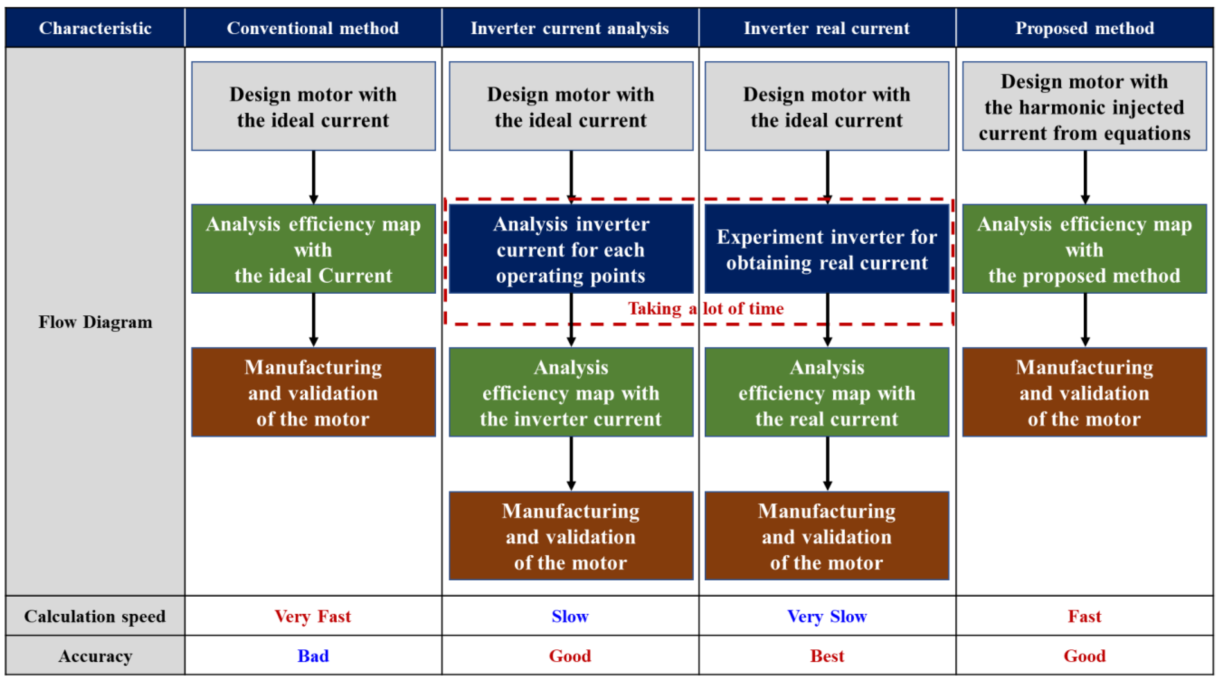
The iron loss of the motor is a factor that is sensitively influenced by the change in the amplitude and frequency of the magnetic flux in stator and rotor cores. Therefore, when harmonic components of the input current are reflected, it is possible to obtain an iron loss analysis result with higher accuracy. To reflect harmonic components of the input current, the analysis using actual current data or inverter simulation current data is generally performed. However, such an analysis has a drawback, as it requires a two-step process for the obtainment of the input current to perform the FEA. Characteristic comparison of the conventional methods with the proposed method is shown in Figure 1.

In this study, we propose a technique to improve the accuracy of losses obtained via the analysis and thus minimize the difference between the analysis and experimental results when analyzing the traction motor using FEA, based on the current source analysis. Because the harmonics generated by the inverter switching frequency are not reflected in the analysis of the ideal current source, we injected the harmonics of the inverter switching frequency to the analysis model to reduce the difference between the analysis and experimental models. To verify the effectiveness of the proposed method, the analysis results of the ideal current source and the proposed method were compared to the experimental results of the manufactured model.

2. Overview of the Ideal Current Source Analysis and the Proposed Method

2.1. Comparison of the Ideal Current Source Analysis and the Proposed Method

In general, the current source analysis of a traction motor is conducted using FEA, based on an ideal balanced 3-phase current, whose phase current equations are as follows:

I_a = Asin(2πft)

(1)

I_b = Asin(2πft + 120°)

(2)

I_c = Asin(2πft − 120°)

(3)

where I_a, I_b, and I_c are the input currents of each phase. A and f denote the amplitude and frequency of the input current, respectively.

The equations for the current source in which harmonics are injected are as follows:

I_ah = A(1 − p^k)sin(2πft) + A_sfpsin(2π(f_sf/f)t)

(4)

I_bh = A(1 − p^k)sin(2πft + 120°) + A_sfpsin(2π(f_sf/f)t + 120°)

(5)

I_ch = A(1 − p^k)sin(2πft − 120°) + A_sfpsin(2π(f_sf/f)t − 120°)

(6)

k = 2.5 (p ≤ 0.3) or 2.8 (0.3 < p ≤ 0.5)

(7)

where A_sf denotes the amplitudes of the switching frequency harmonics; I_ah, I_bh, and I_ch are the harmonic injected currents of each phase; p means a coefficient of harmonic injection within over 0 and under 0.5. For example, the p-value of 0.1 means 10% harmonic injecting. f and f_sf denote the frequencies of the ideal current and the switching frequency harmonics, respectively. k is a constant [11,12,13,14].

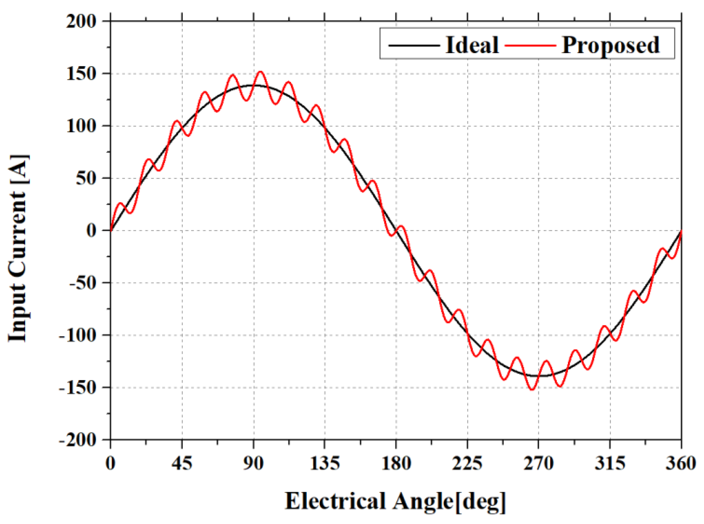
The root mean square (RMS) value of the input current increases when harmonic components are injected into the ideal current source. Thus, we propose an equation to equalize the RMS value of the input current in ideal current source analysis and the proposed method. If the p-value is less than or equal to 0.3, the k-value takes 2.5, and if the p-value is over 0.3 and under 0.5, the k-value gets 2.8. the p-value and k-value are chosen by the designer. Equations (4)–(7) are proposed in this study for simplicity and improvement of analysis based on FEA. The error rate of the RMS current value between the ideal current and the proposed method is a maximum of 0.83%. The p-value in this study was 0.0986, which was chosen from the test result of several traction motors. The comparison of the ideal current analysis and proposed method are shown in Figure 2.

2.2. Modeling and Analysis of the Target Model

The specifications of the target motor and inverter are presented in

Table 1. Specifications of the target motor and inverter.

Category	Unit	Value
Outer diameter	[mm]	280
Magnetic steel sheet	[-]	27PNX1350F
Magnet grade (Br)	[-]	N44 (1.33T)
Maximum input current	[Arms]	205
DC-link voltage	[Vdc]	360
Switching frequency	[Hz]	8000
Maximum Torque	[Nm]	250
Maximum Power	[kW]	50
Maximum Speed	[rpm]	6000

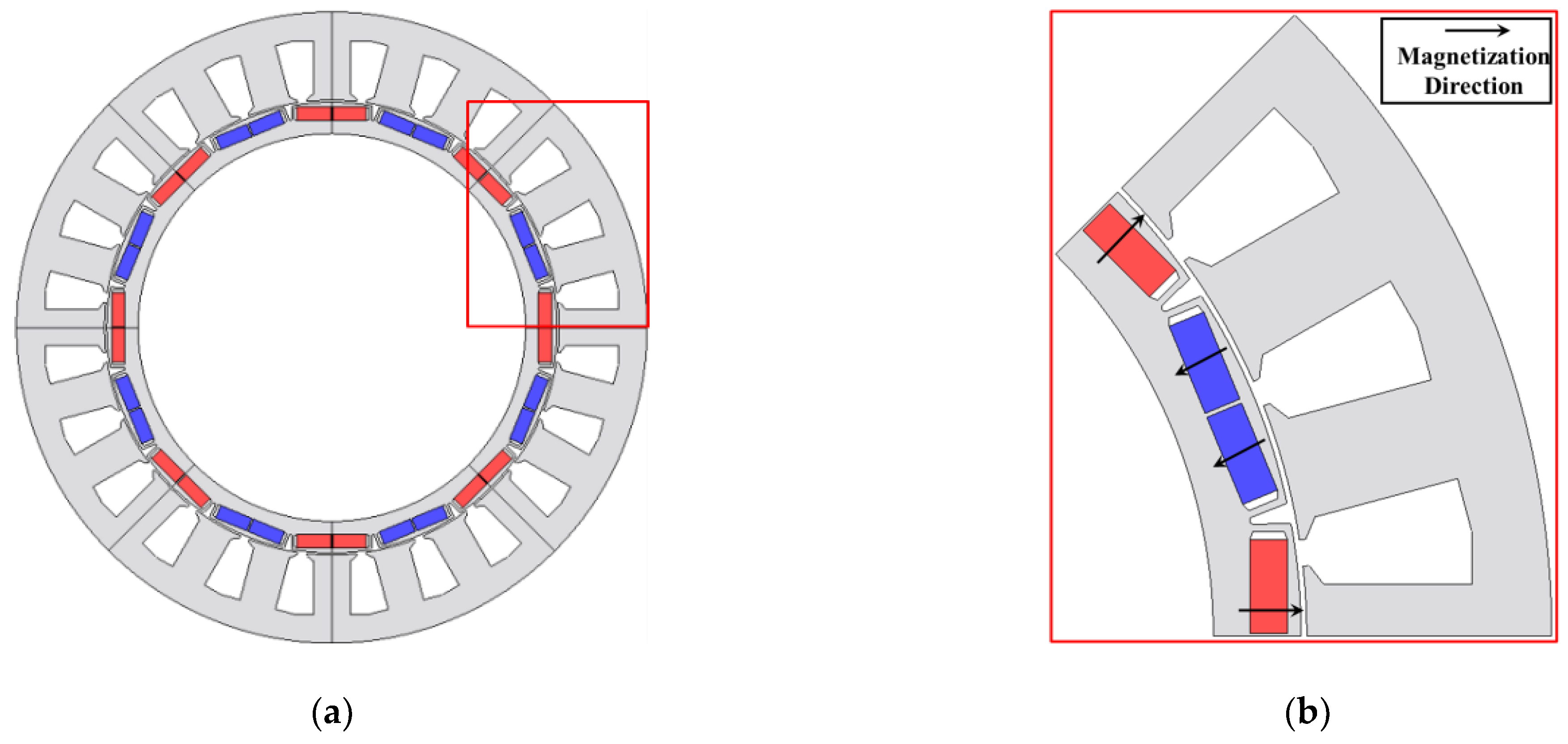
. A traction motor for a hybrid electric vehicle (HEV) was designed according to the specifications presented in Table 1. Considering the maximum speed of the target motor and inverter switching frequency, the number of poles was chosen as 16. In addition, the number of slots was chosen as 24 with concentrated winding to satisfy the high torque density of HEV. The magnetization direction of the designed model was radial.

The topology of the designed model is shown in Figure 3.

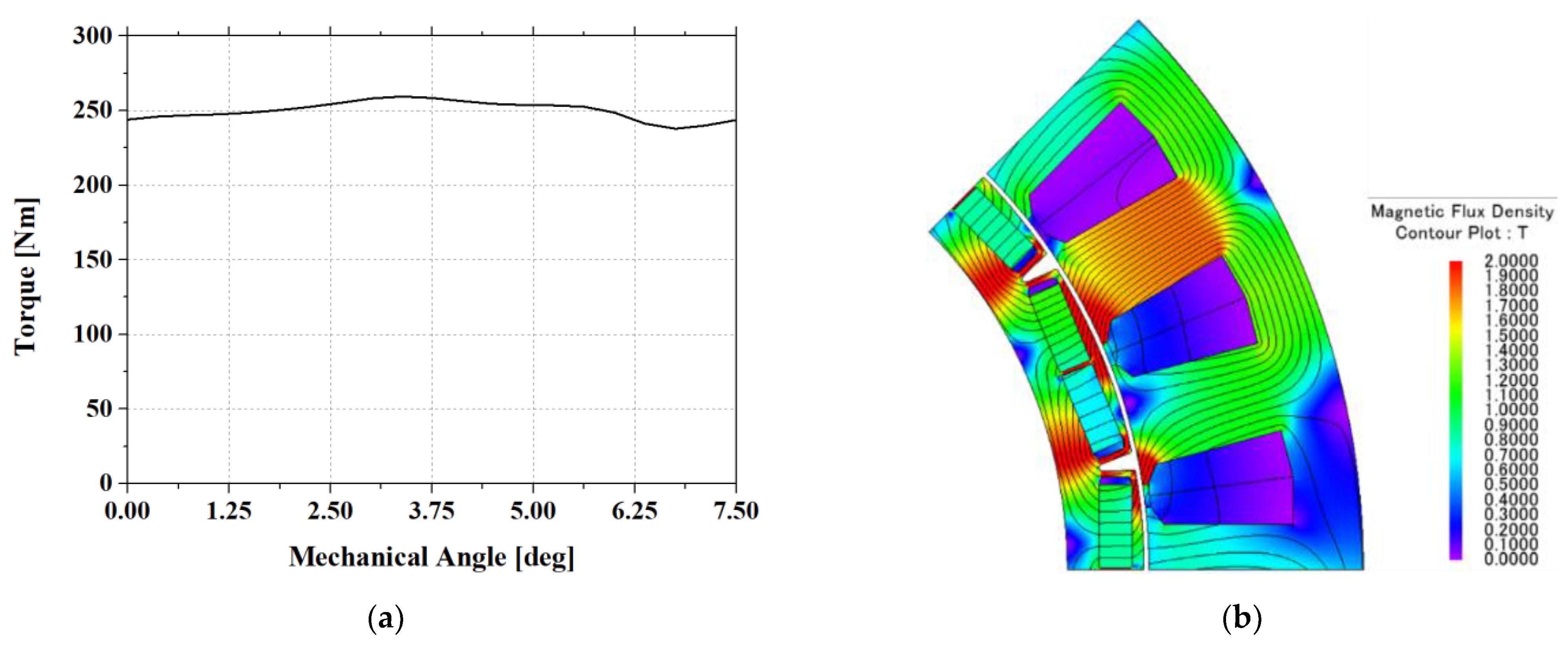
To verify the performance of the designed model, a 2-D FEA analysis of the torque was conducted in load condition, satisfying the target torque and power. Triangular mesh was used the number of mesh elements were 45,626. The waveform of the torque and the magnetic flux density and magnetic flux line of the designed model are shown in Figure 4a,b. According to the FEA analysis in loaded condition, the average torque and output power of the designed model were 250.27 Nm and 50.058 kW, respectively.

2.3. Comparison of Loss Analysis Using the Ideal Current Source and the Proposed Method

The loss analysis of an ideal current source is compared to that of the proposed method, which is based on the injection of harmonics of an inverter switching frequency to the ideal current source. Using Equations (1)–(7), the current sources were generated and used for the loss analysis.

The motor loss is largely classified into copper, iron, and mechanical losses. First, the equation for the copper loss is as follows [15]:

P_copper = nI²R

(8)

where n denotes the number of phases, I is the RMS value of the input current, and R is the resistance of the phase. According to Equation (8), because the copper loss considers the RMS value of the input current, the total copper loss of the ideal current source is similar to that of the proposed method.

Second, the equation for the iron loss is as follows [16,17,18]:

P_iron = P_h + P_e

(9)

P_h = k_hfB^m (1.5 < m < 2.5)

(10)

P_e = k_ef²B²

(11)

where P_h and P_e denote the hysteresis and eddy-current losses, respectively; k_h is the coefficient of the hysteresis loss; m is an empirically determined constant; k_e is the coefficient of the eddy-current; f is the frequency; and B is the magnetic flux density.

According to Equations (9) and (10), P_iron is affected by the frequency and magnetic flux density. Therefore, if the analysis of the iron loss is performed in the frequency domain using fast Fourier transform (FFT), different values will be obtained for the total iron loss for the analysis of the ideal current source and the proposed method [19,20].

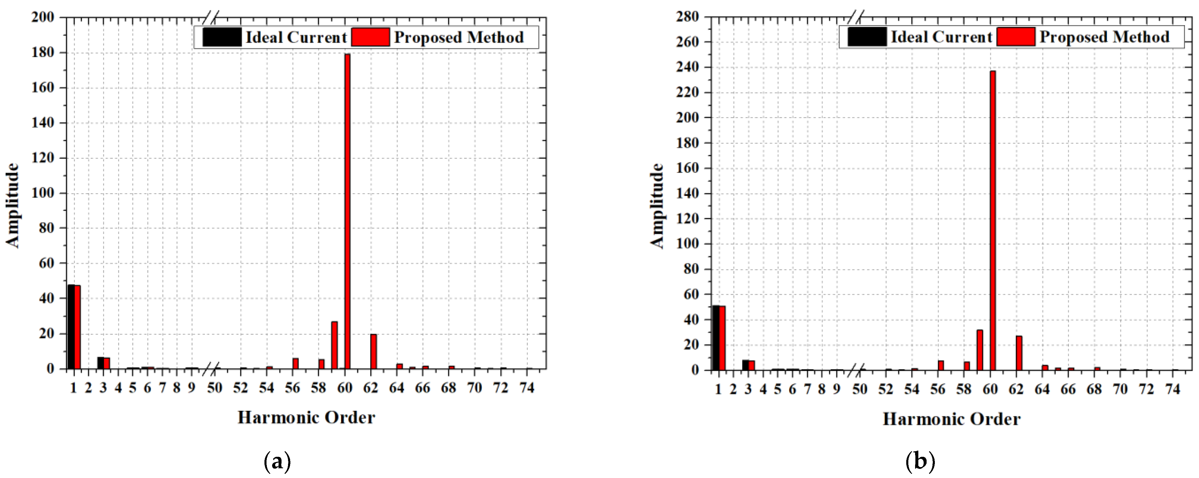
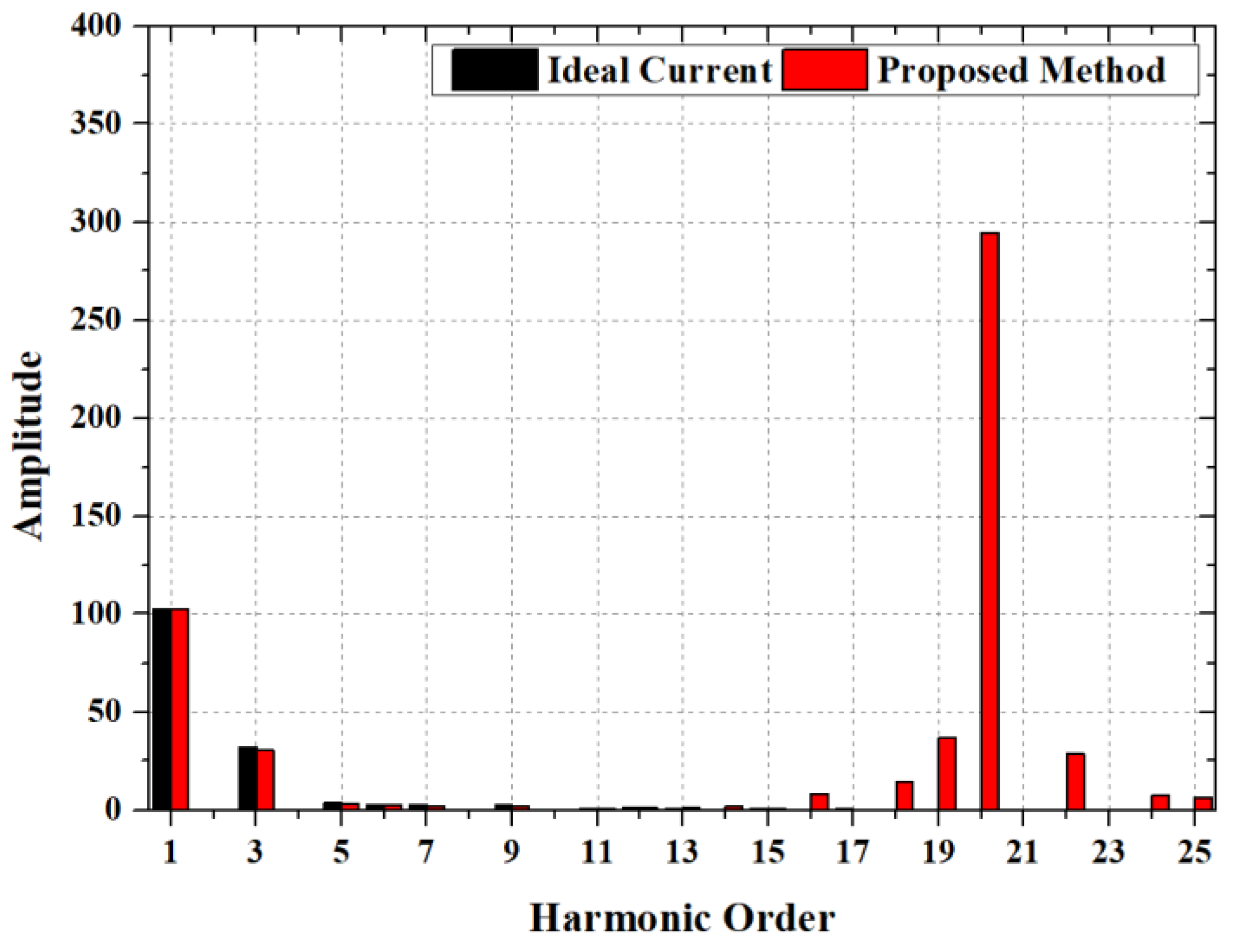
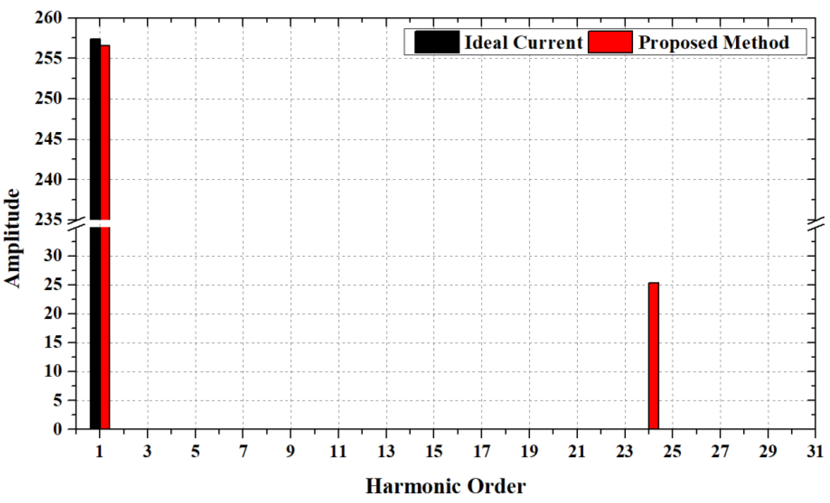
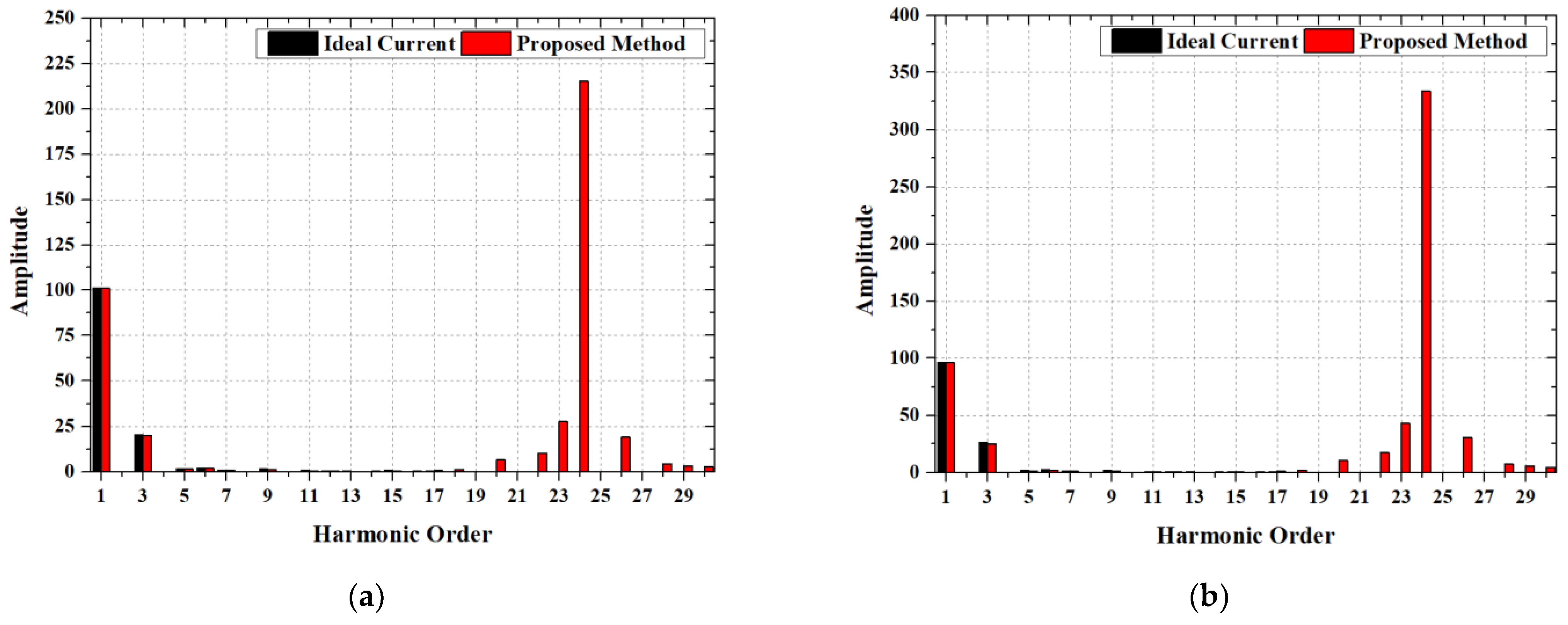
The FFT plot of the ideal current source and the proposed method is shown in Figure 5, where the x-axis and y-axis denote the frequency and amplitude of the input current, respectively. Figure 5 confirms that the proposed method has approximately 25.38 A current at 8000 Hz switching frequency. However, the ideal current source does not have any other harmonics.

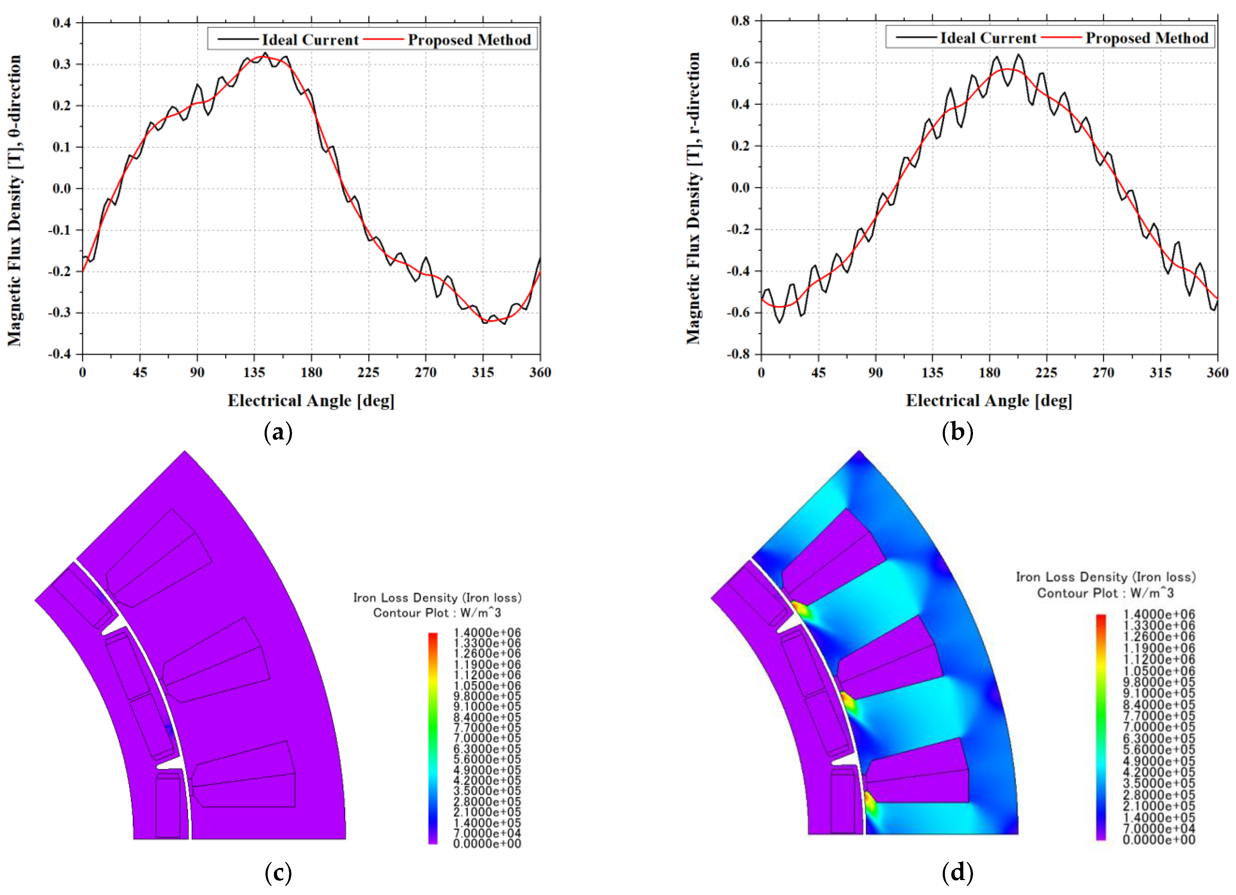
In the proposed method, the harmonic components are applied to the current source, which distorts the average magnetic flux density of every elements in the stator core. Figure 6a,b show the magnetic flux density in the θ and r direction. Therefore, the iron loss analyzed in the frequency domain at 8000 Hz was also affected by those harmonics. The iron loss density at 8000 Hz are shown in Figure 6c,d [21].

3. Experimental Results of the Proposed Method

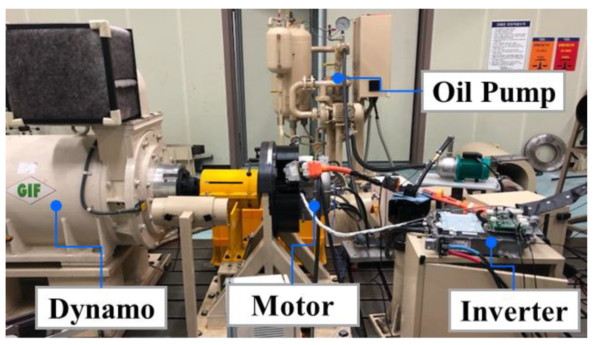
To verify the effectiveness of the proposed method, the experimental model was manufactured and tested using a motor dynamometer. Figure 7 shows the experimental setup.

First, the operating points, which are the main operating points of the traction motor for a hybrid vehicle in the vehicle driving performance simulation, were chosen to conduct the experiment. The chosen operating points are presented in

Table 2. Operating points for the experiment.

Case Number	Torque [Nm]	Speed [rpm]
1	125	1000
2	155	1000
3	100	2500
4	125	2500
5	99	3000

.

Second, a no-load test was conducted to obtain the mechanical losses. The results are summarized in

Table 3. Mechanical losses in the no-load condition.

Speed [rpm]	Mechanical Loss [W]
1000	20.94
2500	119.9
3000	166.5

.

Finally, the efficiency of the motor was defined, and the experiment was conducted in loaded condition. The equation for the efficiency is as follows:

η = P_out/P_in = Tω_m/(Tω_m + P_copper + P_iron + P_mech)

(12)

where P_out and P_in denote the output and input power of the motor, respectively; T and ω_m are the torque and mechanical angular velocity, respectively; and P_mech is the mechanical loss of the motor.

The efficiency based on the ideal current source and the proposed method were compared to the experimental data. The comparison results for each operating point are discussed below.

Table 4. Case 1: 125 Nm at 1000 rpm.

Method	Irms [A]	Copper Loss [W]	IronLoss [W]	Mech Loss [W]	Efficiency [%]
Ideal current source analysis	81.9	543.9	60.1	20.94	95.4
Proposed method	82.2	547.6	305.99	20.94	93.7
Experimental data	81.9	543.9	393.5 (expected)	20.94	93.2

and

Table 5. Case 2: 155 Nm at 1000 rpm.

Method	Irms [A]	Copper Loss [W]	Iron Loss [W]	Mech Loss [W]	Efficiency [%]
Ideal current source analysis	102.9	858.0	65.5	20.94	94.5
Proposed method	103.3	863.9	387.53	20.94	92.7
Experimental data	102.9	858.0	477.0 (expected)	20.94	92.3

present the results for cases 1 and 2, respectively.

For cases 1 and 2, the difference in efficiency between the ideal current source analysis results and the experimental data were 2.2%. However, the differences in efficiency between the proposed method results and the experimental data were 0.5% and 0.4% for case 1 and 2, respectively. In both cases, as the speed of the motor is low, the motor output power is also low. Therefore, the iron loss significantly reduces the efficiency. The iron loss comparison between the ideal current source analysis and the proposed method for cases 1 and 2 is shown in Figure 8.

Table 6. Case 3: 100 Nm at 2500 rpm.

Method	Irms [A]	Copper Loss [W]	Iron Loss [W]	Mech Loss [W]	Efficiency [%]
Ideal current source analysis	81.6	539.7	130.7	119.9	97.1
Proposed method	81.9	543.4	429.1	119.9	96.0
Experimental data	81.6	539.7	402.9 (expected)	119.9	96.1

and

Table 7. Case 4: 125 Nm at 2500 rpm.

Method	Irms [A]	Copper Loss [W]	Iron Loss [W]	Mech Loss [W]	Efficiency [%]
Ideal current source	107.6	937.7	134.2	119.9	96.5
Proposed method	107.9	944.1	600.9	119.9	95.2
Experimental data	107.6	937.7	506.8 (expected)	119.9	95.5

present the results for cases 3 and 4, respectively.

For cases 3 and 4, the differences in efficiency between the ideal current source analysis results and the experimental data was 1.0%. However, the differences in efficiency between the proposed method results and the experimental data were −0.1% and −0.3%, respectively. The iron loss values obtained via the proposed method were approximately 3.28 and 4.47 times higher than those obtained via the ideal current source analysis for cases 3 and 4, respectively. The iron loss comparison between the ideal current source analysis and the proposed method in cases 3 and 4 is shown in Figure 9.

Table 8. Case 5:. 99 Nm at 3000 rpm.

Method	Irms [A]	Copper Loss [W]	Iron Loss [W]	Mech Loss [W]	Efficiency [%]
Ideal current source	98.3	782.9	150.4	166.5	96.6
Proposed method	98.6	788.2	564.4	166.5	95.3
Experimental data	98.3	782.9	785.2 (expected)	166.5	94.7

presents the results for case 5.

In case 5, the difference in efficiency between the ideal current source analysis results and the experimental data was 1.6%, whereas the difference between the proposed method results and the experimental data was 0.6%.

The iron loss comparison between the ideal current source analysis and the proposed method in case 5 is shown in Figure 10.

4. Conclusions

In this study we have proposed a numerical method for improving the accuracy of the iron loss analysis. In general, because the analysis of the ideal current source used in the analysis of the motor does not reflect the harmonics of the inverter switching frequency, the accuracy of analysis of iron loss affected by harmonics is low. To improve this accuracy, we proposed a method in which the harmonics of the inverter switching frequency was injected to the current source.

To verify our method, a traction motor for an HEV was designed, and load analyses using the ideal current source and the proposed method (with harmonics injected current source) were conducted. To guarantee the accuracy of the analysis, a characteristic analysis based on FEA was conducted, and the results confirmed that the proposed method presented a higher iron loss value than the ideal current source analysis at a switching frequency of 8000 Hz.

In addition to the analysis, an experimental model was built and tested. Efficiency tests of the traction motor were performed at five main operating points derived from the vehicle driving performance simulation. The results were compared with those of the ideal current source analysis and the proposed method to verify the effectiveness of the proposed method. The results revealed that the proposed method presented a lower difference in efficiency (difference from simulation) than the ideal current source analysis at all operating points analyzed, and the average efficiency differences of the ideal current source analysis and the proposed method at all operating points were 1.67% and 0.25%, respectively. In the future, we shall propose a novel method that offers a higher accuracy in loss calculation than the method proposed in this study, using peripheral harmonics of the switching frequency.

References

- Jafari, M.; Gauchia, A.; Zhao, S.; Zhang, K.; Gauchia, L. Electric Vehicle Battery Cycle Aging Evalu-ation in Real-World Daily Driving and Vehicle-to-Grid Services. IEEE Trans. Transp. Electrif. 2018, 4, 122–134. [Google Scholar] [CrossRef]
- Lam, A.Y.S.; Leung, K.-C.; Li, V.O.K. Capacity Estimation for Vehicle-to-Grid Frequency Regulation Services With Smart Charging Mechanism. IEEE Trans. Smart Grid 2015, 7, 156–166. [Google Scholar] [CrossRef] [Green Version]
- Horrein, L.; Bouscayrol, A.; Lhomme, W.; Depature, C. Impact of Heating System on the Range of an Electric Vehicle. IEEE Trans. Veh. Technol. 2016, 66, 4668–4677. [Google Scholar] [CrossRef]
- Lee, D.-K.; Ro, J.-S. Analysis and Design of a High-Performance Traction Motor for Heavy-Duty Vehicles. Energies 2020, 13, 3150. [Google Scholar] [CrossRef]
- Lim, D.-K.; Ro, J.-S. Analysis and Design of a Delta-Type Interior Permanent Magnet Synchronous Generator by Using an Analytic Method. IEEE Access 2019, 7, 85139–85145. [Google Scholar] [CrossRef]
- Song, J.-Y.; Lee, J.H.; Kim, D.-W.; Kim, Y.-J.; Jung, S.-Y. Analysis and Modeling of Permanent Magnet Variable Flux Memory Motor Using Magnetic Equivalent Circuit Method. IEEE Trans. Magn. 2017, 53, 1–5. [Google Scholar] [CrossRef]
- Liu, Y.; Zhang, Z.; Geng, W.; Li, J. A Simplified Finite-Element Model of Hybrid Excitation Synchronous Machines With Radial/Axial Flux Paths via Magnetic Equivalent Circuit. IEEE Trans. Magn. 2017, 53, 1–4. [Google Scholar] [CrossRef]
- Yoon, H.; Song, M.; Kim, I.; Shin, P.S.; Koh, C.S. Accuracy Improved Dynamic E&S Vector Hysteresis Model and its Application to Analysis of Iron Loss Distribution in a Three-Phase Induction Motor. IEEE Trans. Magn. 2012, 48, 887–890. [Google Scholar] [CrossRef]
- Zhang, D.; Liu, T.; Zhao, H.; Wu, T. An Analytical Iron Loss Calculation Model of Inverter-Fed In-duction Motors Considering Supply and Slot Harmonics. IEEE Trans. Idust. Electron. 2019, 66, 9194–9204. [Google Scholar] [CrossRef]
- Yamazaki, K.; Sato, Y.; Domenjoud, M.; Daniel, L. Iron Loss Analysis of Permanent-Magnet Machines by Considering Hysteresis Loops Affected by Multi-Axial Stress. IEEE Trans. Magn. 2019, 56, 1–4. [Google Scholar] [CrossRef]
- Takada, S.; Mohri, K.; Takito, H.; Nomura, T.; Sasaki, T. Magnetic losses of electrical iron sheet in squirrel-cage induction motor driven by PWM inverter. IEEE Trans. Magn. 1997, 33, 3760–3762. [Google Scholar] [CrossRef]
- Lee, G.-H.; Kim, S.-I.; Hong, J.-P.; Bahn, J.-H. Torque Ripple Reduction of Interior Permanent Magnet Syn-chronous Motor Using Harmonic Injected Current. IEEE Trans. Magn. 2008, 44, 1582–1585. [Google Scholar]
- Li, G.-J.; Zhang, K.; Zhu, Z.Q.; Jewell, G. Comparative Studies of Torque Performance Improvement for Different Doubly Salient Synchronous Reluctance Machines by Current Harmonic Injection. IEEE Trans. Energy Convers. 2019, 34, 1094–1104. [Google Scholar] [CrossRef]
- Zhang, H.; Liu, W.; Chen, Z.; Luo, G.; Liu, J.; Zhao, D. Asymmetric Space Vector Modulation for PMSM Sensorless Drives Based on Square-Wave Voltage-Injection Method. IEEE Trans. Ind. Appl. 2018, 54, 1425–1436. [Google Scholar] [CrossRef]
- Luo, C.; Sun, J.; Liao, Y.; Xu, S. Analysis and Design of Ironless Toroidal Winding of Tubular Linear Voice Coil Motor for Minimum Copper Loss. IEEE Trans. Plasma Sci. 2019, 47, 2369–2375. [Google Scholar] [CrossRef]
- Yamazaki, K.; Fukushima, N. Iron-Loss Modeling for Rotating Machines: Comparison Between Bertotti’s Three-Term Expression and 3-D Eddy-Current Analysis. IEEE Trans. Magn. 2010, 46, 3121–3124. [Google Scholar] [CrossRef]
- Yamazaki, K.; Takaki, Y. Iron Loss Analysis of Permanent Magnet Motors by Considering Minor Hysteresis Loops Caused by Inverters. IEEE Trans. Magn. 2019, 55, 1–4. [Google Scholar] [CrossRef]
- Seo, M.-K.; Ko, Y.-Y.; Lee, T.-Y.; Kim, Y.-J.; Jung, S.-Y. Loss Reduction Optimization for Heat Ca-pacity Improvement in Interior Permanent Magnet Synchronous Machine. IEEE Trans. Magn. 2018, 54, 1–5. [Google Scholar]
- Kadjoudj, M.; Benbouzid, M.E.H.; Ghennai, C.; Diallo, D. A Robust Hybrid Current Control for Permanent-Magnet Syn-chronous Motor Drive. IEEE Trans. Energy Convers. 2004, 19, 109–115. [Google Scholar] [CrossRef]
- Gersem, H.D.; Hameyer, K. Air-gap Flux Splitting for the Time-Harmonic Finite-Element Simulation of Single-phase Induc-tion Machines. IEEE Trans. Magn. 2002, 38, 1221–1224. [Google Scholar] [CrossRef]
- Chang, L.; Jahns, T.M.; Blissenbach, R. Estimation of PWM-Induced Iron Loss in IPM Machines Incorporating the Impact of Flux Ripple Waveshape and Nonlinear Magnetic Characteristics. IEEE Trans. Ind. Appl. 2020, 56, 1332–1345. [Google Scholar] [CrossRef]
Figure 1.
Characteristic comparison of the conventional methods with the proposed method.
Figure 2.
Comparison of the ideal current and the harmonics injected current source.
Figure 3.
Topology of the designed model. (a) Full designed model; (b) Periodic part of the designed model.
Figure 4.
Waveform of torque, magnetic flux density, and magnetic flux line of the designed model in load condition. (a) Torque waveform of the designed model; (b) Magnetic flux density of the designed model.
Figure 5.
FFT plot of the ideal and harmonics injected currents.
Figure 6.
Comparison of magnetic flux and iron loss densities. (a) Magnetic flux density of in the stator core: θ-direction; (b) Magnetic flux density in the stator core: r-direction; (c) Iron loss density at 8000 Hz (ideal current source); (d) Iron loss density at 8000 Hz (proposed method).
Figure 7.
Experimental setup.
Figure 8.
Iron loss comparison between the ideal current source analysis and the proposed method for cases 1 and 2. (a) Case 1. (b) Case 2.
Figure 9.
Iron loss comparison between the ideal current source analysis and the proposed method for cases 3 and 4. (a) Case 3; (b) Case 4.
Figure 10.
Iron loss comparison between the ideal current source analysis and the proposed method in case 5.