Abstract
In this paper, it is shown how the performance of the monopulse algorithm in the presence of an additive noise can be obtained analytically. In a previous study, analytic performance analysis based on the first-order Taylor series and the second-order Taylor series was conducted. By adopting the third-order Taylor series, it is shown that the analytic performance based on the third-order Taylor series can be brought closer to the performance of the original monopulse algorithm than the analytic performance based on the first-order Taylor series and the second-order Taylor series.
1. Introduction
A radar measures the distance, direction, and speed information of a target using electromagnetic waves and can perform search and tracking functions. The search mode explores a given volume space in the absence of information about the target and detects the target. When a target is detected, the tracking mode is activated. In this case, the target is tracked while measuring states such as distance, angle, and speed. Amplitude-comparison monopulse radar (ACM) is classified as tracking radar, and it is possible to accurately measure the tracking error of a target with only one pulse (monopulse). The monopulse radar-receiving antenna consists of four receiving beam patterns with the same squint angle. The received signals are incident on the four receiving beam patterns, and the signals incident on the receiving antenna are inputted through the sum channel and the difference channels. The azimuth and elevation tracking error are calculated through the signal amplitude ratio of these channels [1,2,3].
In [4,5,6], many methods were proposed to improve the angular performance of the monopulse radar. In [4], the angle of the target was estimated using multiple antennas in the amplitude comparison monopulse radar. Although the amplitudes of the signal received by each antenna vary according to the angle of the target, it is assumed that the arrival time of the signals are the same. The generalized likelihood ratio test is used to express the detection and parameter-estimation method for the radar receiver. In [5], an adaptive array for estimated angle was used. The maximum likelihood theory was applied to sum and difference monopulse beams that suppress external noise sources. In addition, their method was shown to perform well in the presence of side lobe and main beam interference. In [6], the author dealt with the DOA resolution problem of two targets in the four-channel monopulse radar and proposed a new solution to solve them.
The proposed methods of the above-mentioned papers mainly dealt with improving the angle estimation performance of monopulse radar. In this regard, we analyze and compare the angle estimation performance of the methods proposed in the above papers in detail with various noises. Therefore, methods to efficiently and accurately calculate the estimated angle MSE under the influence of various noises are studied.
In general, the return signal and noise are received by the receiving antenna [7]. Noise is caused by several environmental variables (interference and propagation effects). In the ACM, this noise has a great influence on the ability to estimate the angular position of the target. Therefore, it is necessary to calculate the target angle estimation accuracy by explicitly analyzing the angle estimation error caused by additive noise to the actual incident angle of the ACM.
Previously, studies on the performance analysis of monopulse radar have been conducted in a similar manner. In [8,9,10,11], the authors dealt with the performance analysis of the angle estimation of monopulse radar. In [8], the author considered the performance of the monopulse receiver in relation to the cause of the internal error. Four main types of monopulse receivers were analyzed, and an analysis was performed based on a mathematical model. However, external errors were excluded. In [9], the estimated angle performance of a monopulse radar with receiving inconsistency was analyzed. In the estimated angle performance, it was shown that not only the algorithm but also the amplitude-phase mismatch affects the estimated angle performance. However, performance analysis considering various measurement noises was not conducted. In [10], the author dealt with the angle estimation problem of ACM radar when thermal noise is present internally. Similarly, performance analysis on the influence of external measurements was not performed. In [11], the authors presented the ACM algorithm and the covariance prediction equation. The proposed covariance equation was simple, but it predicted the RMS error very accurately.
Most of the papers considered only the influence of internal noise and did not consider the measurement noise caused by external variables. In this regard, we previously conducted a performance analysis of the ACM radar considering external noise. In a previous study [12], the MSE of the ACM Direction-of-Arrival (DOA) estimated angle was expanded as an analytic expression using the first-order Taylor approximation and the second-order Taylor approximation and compared with the Monte-Carlo method. In order to improve the analytic MSE of the second-order Taylor approximation in [12], we propose an analytic MSE of the third-order Taylor approximation.
In this paper, we focus on improving the accuracy of the analytic expression of the estimated angle MSE of the ACM algorithm using the first-order Taylor approximation and the second-order Taylor approximation proposed in the previous study [12]. Therefore, we improve the MSE calculation accuracy of the estimated angle considering noise through the third-order Taylor approximation of the analytic expression. In order to analyze the accuracy of angle estimation under various noise effects, studies are conducted in the case of several standard deviations. The MSE of the ACM angle estimation algorithm is derived through Monte-Carlo simulation, and the MSE is analytically derived using the third-order Taylor approximation. In addition, we confirm that the computational complexity of the analytic MSE is lower than that of the MSE based on Monte-Carlo method.
In Section 2.1, the angle estimation principle of ACM radar is described. In Section 2.2, angle estimation equations of the ACM radar considering additive noise are derived. In Section 2.3, the simulation MSE and analytic MSE are defined. In Section 3, the performances of analytic MSEs and simulation MSEs are analyzed. In addition, the errors of the analytic MSEs of the second-order Taylor approximation are improved by using the analytic MSEs of the third-order Taylor approximation. In the Appendix, the analytic MSEs of the third-order Taylor approximation are derived.
2. Methodologies
2.1. Estimated Angle Error of the Amplitude-Comparison Monopulse Radar
In this subsection, we describe the angle principle of ACM radar to derive the angle estimation equations under the effect of additive noise.
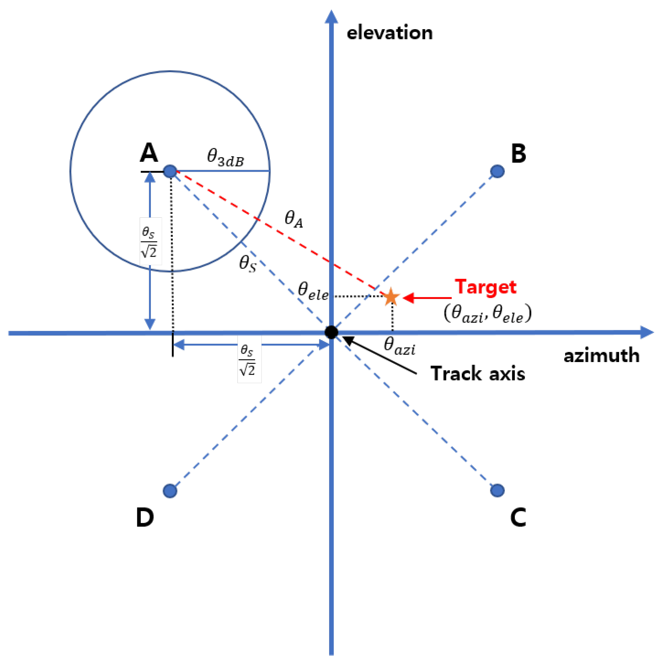
A monopulse radar is a tracking radar that measures the angle (tracking error) through only one pulse. The angle estimation principle of monopulse radar can be divided into a phase-comparison method and an amplitude-comparison method. In this paper, amplitude-comparison monopulse radar is used, and it is assumed that it has four squinted receive beams and three channels. The ACM radar receives an incident signal using squinted beams. The amplitudes of the incident signal are input to the sum channel and difference channels, and the tracking error is estimated through the output of these channels [3]. Figure 1 briefly shows the tracking error of the target from the tracking center of the monopulse radar. The track axis means the central axis for the radar to track the target. Beams with four boresights have the same squint angle from the track axis. In Figure 1, the tracking error of the target is shown by , . These tracking errors are obtained by comparing the received signal amplitudes of the four beams. In Figure 1, A, B, C, and D denote squinted beams in four different directions. Also, these beams have the same squint angle to each other. When receiving the signal returned from the target, the azimuth tracking error () is obtained through the ratio of the difference between the (A + D) signal and the (B + C) signal and the sum of the signals received from the four receiving beams. The elevation tracking error is obtained through the ratio of the difference between the (A + B) received signal and the (C + D) received signal and the sum of the signals received from the four receiving beams.
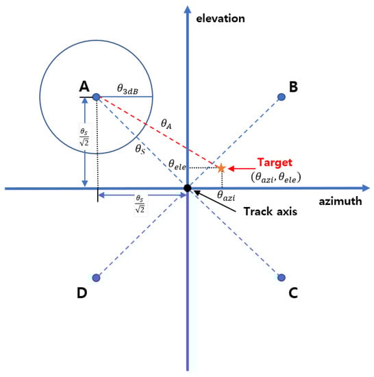
Figure 1.
Tracking center and angle error of monopulse radar.
Assuming that the beam pattern of the monopulse radar antenna is a Gaussian pattern, it is as follows [13]:
where , , and are the angle of the target with respect to the boresight of one beam pattern, the 3 dB beamwidth of one receiving beam, and the gain in the boresight direction of one receiving beam, respectively.
The expression in (1) implies the gain for the received signal incident at a certain angle based on the boresight of one receiving beam. By expanding (1), it is possible to obtain the gain for the target for each of the four receiving beam patterns. The angle of incidence of the target can be expressed in terms of the squint angle (), azimuth tracking error (), and elevation tracking error () as follows [12]:
where , , , and denote the angle of the incident signal based on the receiving beam with a boresight in the A direction, the squint angle, the azimuth tracking error, and the elevation tracking error, respectively.
In general, the target is located close to the track axis. The squares of the azimuth and elevation have a very small value compared to the square of the squint angle. Therefore, it is shown as (3).
By substituting (3) in (1), (1) can be written as [12]
where is replaced by , which denotes the monopulse error slope coefficient. The first approximation in (5) holds due to . The second approximation in (5) is valid since is approximately equal to .
Similarly, , and can be expressed as [14]
The voltage of the incident signal from a specific direction can be obtained by multiplying the gain of each receiving beam from the specific direction and the signal amplitude. The sum pattern and the two difference patterns can be defined. In order to obtain the difference pattern for the azimuth, subtract the (B + C) received signal from the (A + D) received signal, and subtract the (C + D) received signal from the (A + B) received signal to obtain the elevation difference pattern [3]. In (9), and denote the difference channel pattern:
The sum pattern can additionally be obtained by the sum of the received signals for the four beam patterns. In (10), denotes the sum channel pattern:
It is possible to calculate the azimuth estimation error and the elevation estimation error through (9) and (10). (11) is an equation that is used to estimate the tracking error of the signal that is received by the ACM through the sum channel and the difference channel. and mean the estimated tracking error:
2.2. Angle Estimation of Amplitude-Comparison Monopulse Algorithm in Noise Effects Using the Taylor Approximation
Considering the general situation, it is appropriate to add noise for the gain of the received signal for the four receiving beam patterns. In a situation where noise is added, there are several variables, such as thermal noise inside the receiver and noise that is caused by the external environment. In this paper, it is assumed that Gaussian noises, which is not correlated with each other, are added to each received signal.
In (9)–(11), the difference pattern and the sum pattern can be written as [12]
where , , , and denote the noise that is added to the received signal for four beams.
Using (11), the estimated azimuth and estimated elevation are expressed as follows:
where and are the estimated azimuth and the estimated elevation when noise is added, respectively.
In order to obtain (14) and (15), (9) and (10) are used. If the approximation of the received signal gain is not performed, the equation is as follows:
and are the estimated angles (tracking errors) of the actual ACM. and are the resulting values that appear when the output value of (1) is input to the difference channel. is the resulting value that appears when the output value of (1) is input to the sum channel.
Equations (14) and (15) are approximated through (3) and (5) in the process of obtaining the gain, but (16) is the estimated angle using the sum channel and the difference channel without any approximation. This equation models the situation in which the actual ACM estimates the angle.
In (14) and (15), , , , and corresponding to noise are random variables. To obtain the MSE, the mean operation is applied to the square of the estimated angle. However, since (14) and (15) are nonlinear functions shown in a fractional form, it is difficult to develop the mean operation analytically. Therefore, by applying Taylor’s approximation, which approximates this function as a polynomial function for , , , and , the analytical expansion of the mean operation is performed.
In Appendix A, the estimated azimuth and the estimated elevation based on the various orders of Taylor expansion are explicitly given. Note that the expression for the first-order Taylor expansion and the second-order Taylor expansion can also be found in [12].
2.3. Analytic Expression of the MSEs of the Estimated Angle of Amplitude-Comparison Monopulse Algorithm
2.3.1. Simulation MSEs
The Mean Square Error (MSE) is one of the approaches used to measure the accuracy of an estimate. As the name implies, the MSE is defined by taking the mean of the squared error of the estimate. The purpose of our study is to calculate the MSE to measure the accuracy of angle estimation in a noise-affected environment, without having to go through the Monte-Carlo simulation of numerous trials, and to accurately calculate it without loss of computation time cost.
The simulation MSEs from the Monte-Carlo method can be obtained as follows:
where and denote an estimated angle, and and denote a true incident angle.
2.3.2. Analytic MSEs
In Appendix B, the analytic expressions of the MSE of the estimated azimuth and the estimated elevation based on the various orders of Taylor expansion are presented. The expressions associated with the first-order Taylor expansion and the second-order Taylor expansion have also been presented in [12].
In Appendix C, it is assumed that the noise random variables , , , and are all zero mean Gaussian random variables and uncorrelated with each other. Under these conditions, the analytic MSEs are derived through the following process:
- 1.
- 2.
- Second, the result of subtracting the true angles from the angle estimation equation of the Taylor approximation is squared;
- 3.
- Third, the results obtained in the second step are expanded and the expectation operators are applied;
- 4.
- Finally, the expectation operations are applied to the Gaussian random variable noises, and the Nth central moment of the Gaussian random variables is adopted to simplify the expression in steps.
The analytic MSEs for azimuth and elevation are expressed as “Analytic ” and “Analytic ”, respectively.
2.4. Setting SImulation Parameters and Labeling MSE Expressions
In Table 1, it can be seen that several MSEs are matched as identifiable labels.

Table 1.
Labels for MSE expressions.
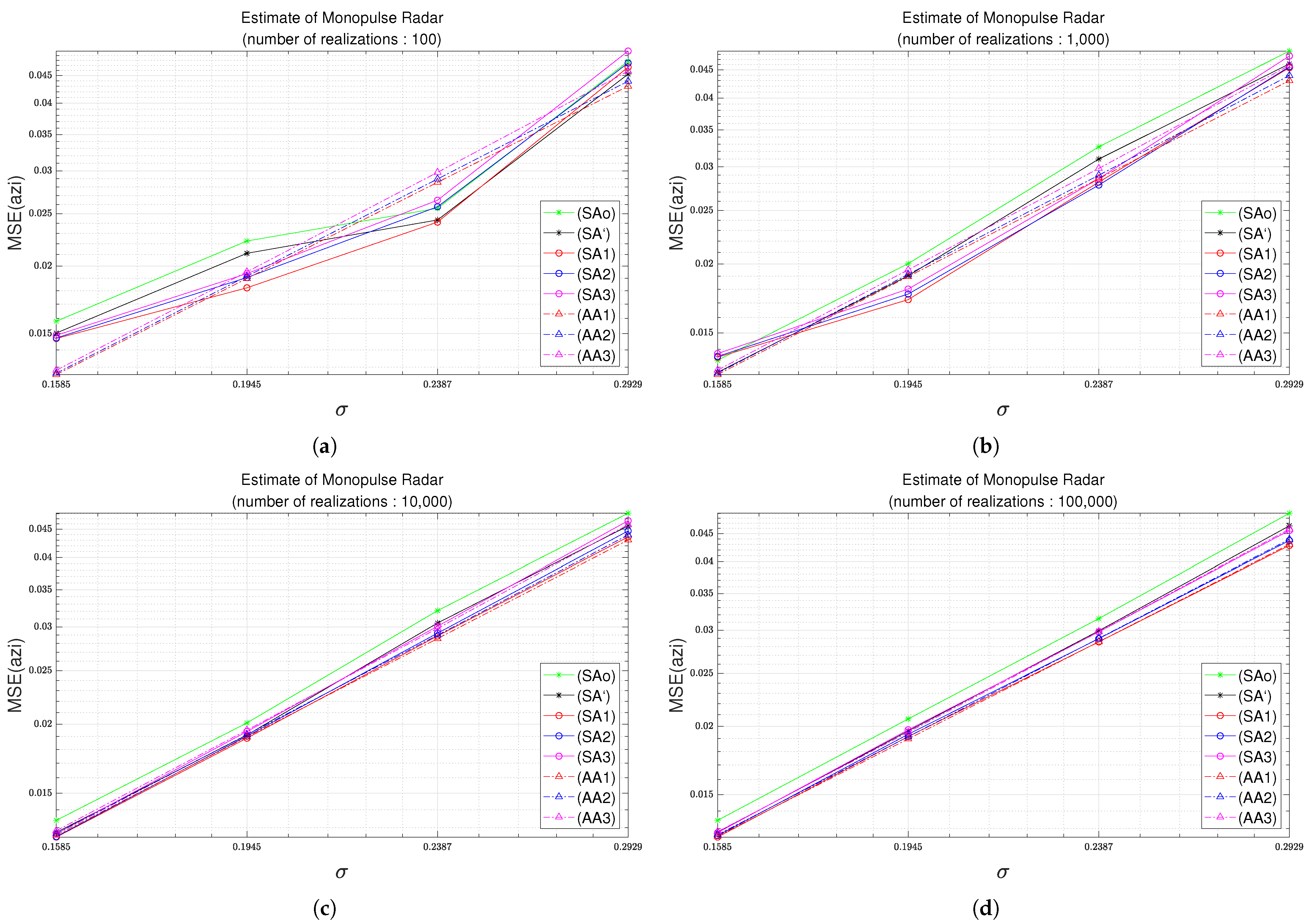
Figure 2 illustrates the MSE results for several numbers of realizations of a Monte-Carlo simulation. Figure 2a–d show the results in terms of the MSEs when the numbers of realizations are 100, 1000, 10,000, and 100,000, respectively. In Figure 2, the results of simulation MSEs such as (SAo), (SA’), (SA1), (SA2), and (SA3) show low accuracy as the number of realizations decreases. It is true that the difference between the simulation-based MSE for 10,000 realizations and the simulation-based MSE for 100,000 realizations is not significant. However, the relative difference of the simulation-based MSE for a number of realizations of 10,000 with respect to the analytically-derived MSE is 1.4%, and the relative difference of the simulation-based MSE for the number of realizations of 100,000 with respect to the analytically-derived MSE is 0.5%.
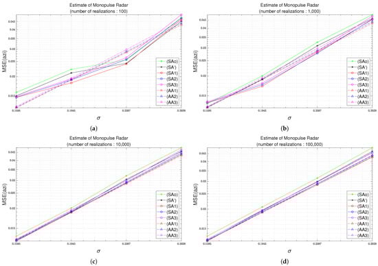
Figure 2.
MSE as a function of standard deviation considering the Monte Carlo simulations with different realization numbers. (a) 100 times. (b) 1,000 times. (c) 10,000 times. (d) 100,000 times.
3. Results
In this section, the performance analysis of analytic MSEs is conducted based on the third-order Taylor approximation. It is verified that the accuracy is improved through a performance comparison with the analytic MSEs of the first and second-order Taylor approximations conducted in the previous study. The performance analysis is performed in a noisy environment with various standard deviations, and the dependence of the MSE on the SNR change is analyzed. The computational complexities of the analytic approach and that of the Monte-Carlo simulation are illustrated, which demonstrates why the proposed analytic approach is useful.
3.1. Test 1: Simulation MSEs and Analytic MSEs
In Table 2, the parameters used in Test 1 are assumed to be as follows:
Table 2.
Parameters for Test 1.
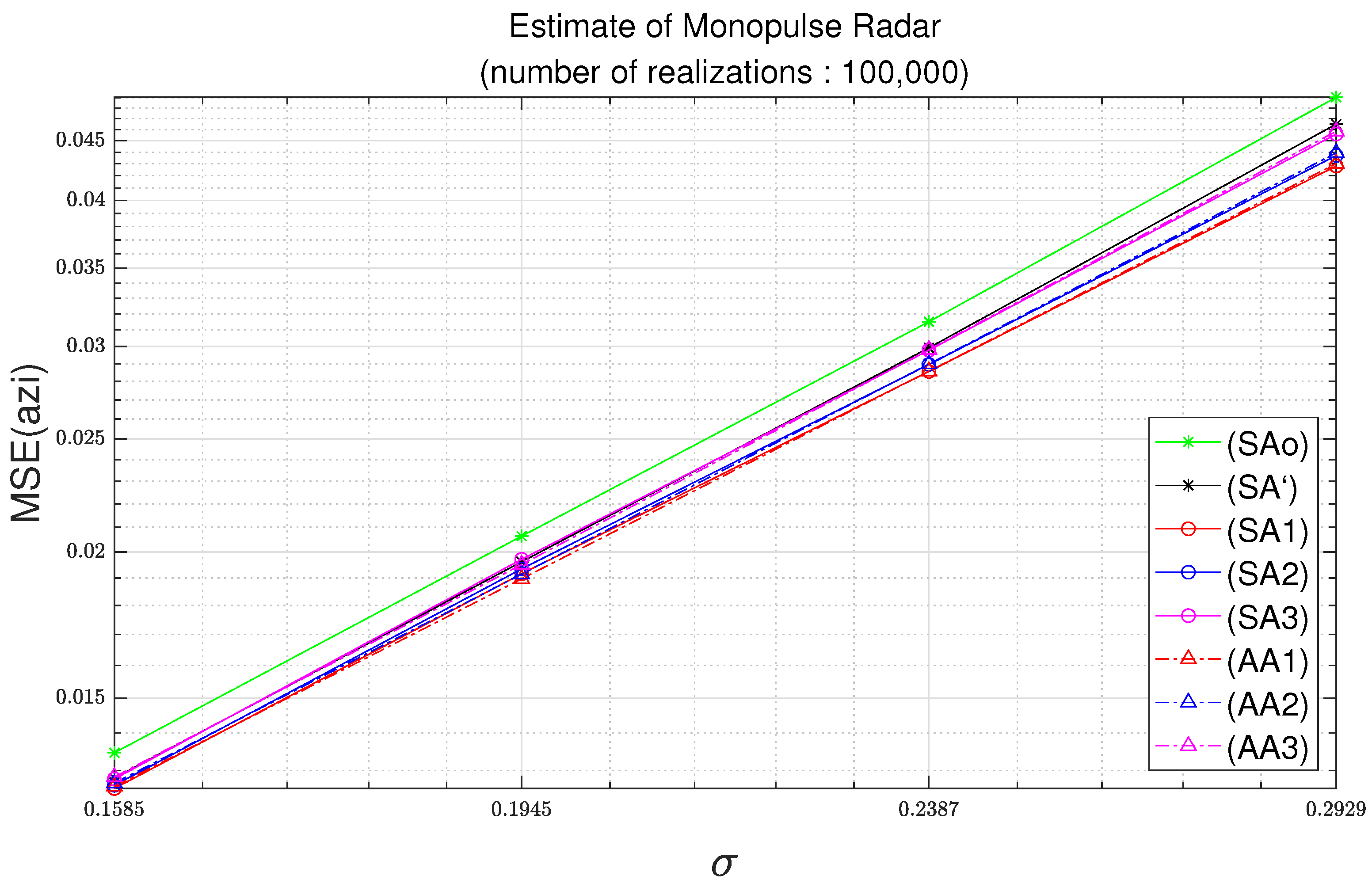
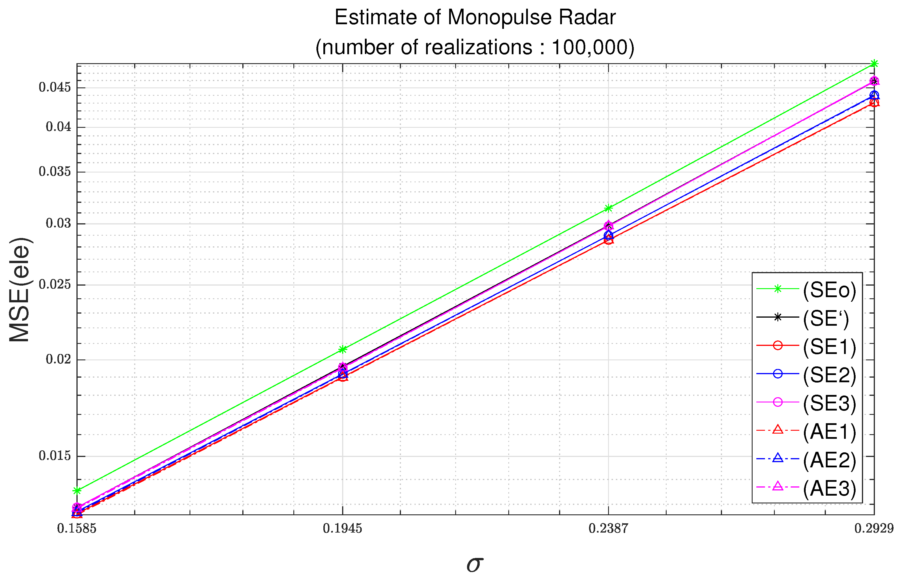
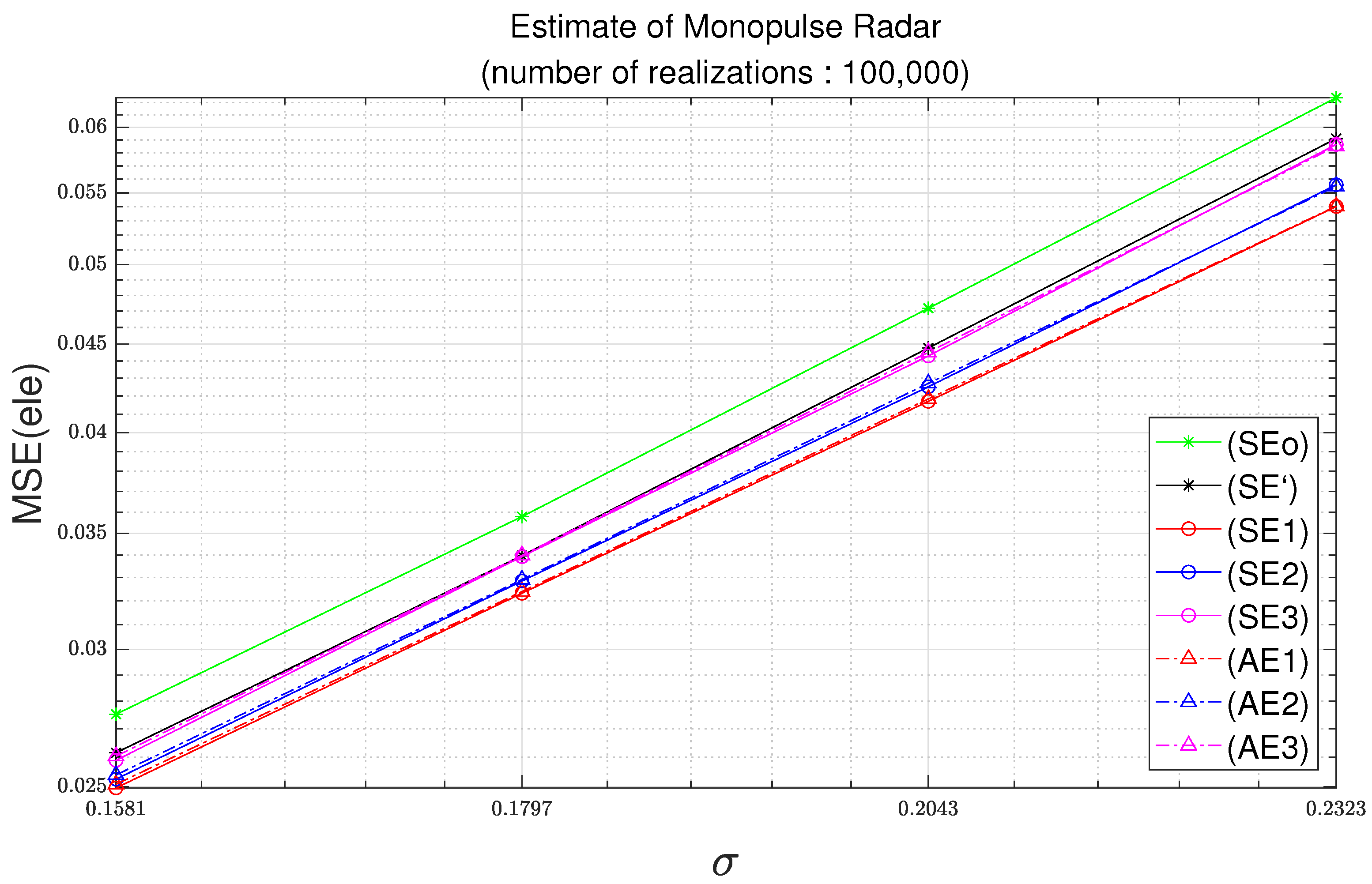
Figure 3 and Figure 4 illustrate the MSEs with respect to the standard deviation of noise with a number of realizations of 100,000. The standard deviation of noise is set to the value specified in Table 2. The standard deviations for , , , and are identical. It is shown in Figure 3 and Figure 4 that the MSEs of the angle estimates increase with the increase of the standard deviation of the additive noise. Figure 3 and Figure 4 illustrate the MSEs for the azimuth and for the elevation, respectively.
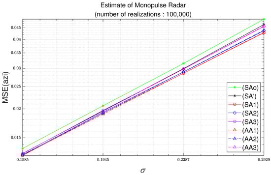
Figure 3.
Azimuth MSE as function of standard deviation with parameters of Table 2 and 100,000 realizations.
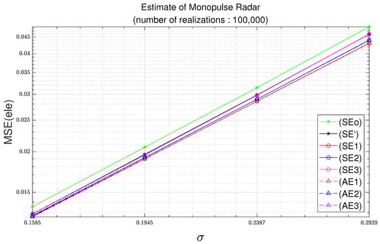
Figure 4.
Elevation MSE as function of standard deviation with parameters of Table 2 and 100,000 realizations.
In Figure 3, empirical MSEs of (SAo), (SA’), (SA1), (SA2), and (SA3) are calculated from (17). In Figure 3, the result with legend (SAo) is obtained from (16), and the result with legend (SA’) is obtained from (14). In Figure 3, the angle estimation equation used for (SA1) is (A10), and the angle estimation equation used for (SA2) is (A12). Similarly, the angle estimation equation used for (SA3) is (A14). In Figure 3, the result with legend (AA1) is obtained from (A33), and the result with legend (AA2) is obtained from (A35). Similarly, the result with legend (AA3) is obtained from (A37).
When comparing the (SAo) and (SA’) in Figure 3, there is a slight difference in the MSE. The reason for this difference is that (SA’) is obtained using the approximations in (3) and (5). For the result with legend (SA1), it can be seen that it is located at the bottom of the result with legend (SA’). The reason is that the first-order Taylor approximation is used to obtain (SA1) from (SA’). The result with legend (SA2) is located closer to the (SA’) than the (SA1). However, there is still a difference between (SA’) and (SA2). Similarly, the reason is that the second-order Taylor approximation is used to obtain (SA2) from (SA’). For the result with legend (SA3), it is illustrated that (SA3) is closer to (SA’) than (SA1) and (SA2). It also seems to almost overlap with (SA’).
Monte-Carlo simulation-based MSEs have been described. Next, how analytic MSEs can be obtained is described. In Figure 3, (AA1) and (AA2) are the results based on the first-order Taylor expansion and the second-order Taylor expansion, respectively. (AA1) and (AA2) show good agreements with (SA1) and (SA2), respectively. Similarly, (AA3) is the result based on the third-order Taylor expansion. (AA3) shows good agreement with (SA3).
In Figure 4, empirical MSEs of (SEo), (SE’), (SE1), (SE2), and (SE3)’ are calculated from (18). In addition, (SEo), (SE’), (SE1), (SE2), and (SE3) are obtained from (15), (16), (A11), (A13) and (A15), respectively. In Figure 4, analytical MSEs (AE1), (AE2), and (AE3) are obtained from (A34), (A36) and (A38), respectively. The observations in Figure 3 can also be found in Figure 4.
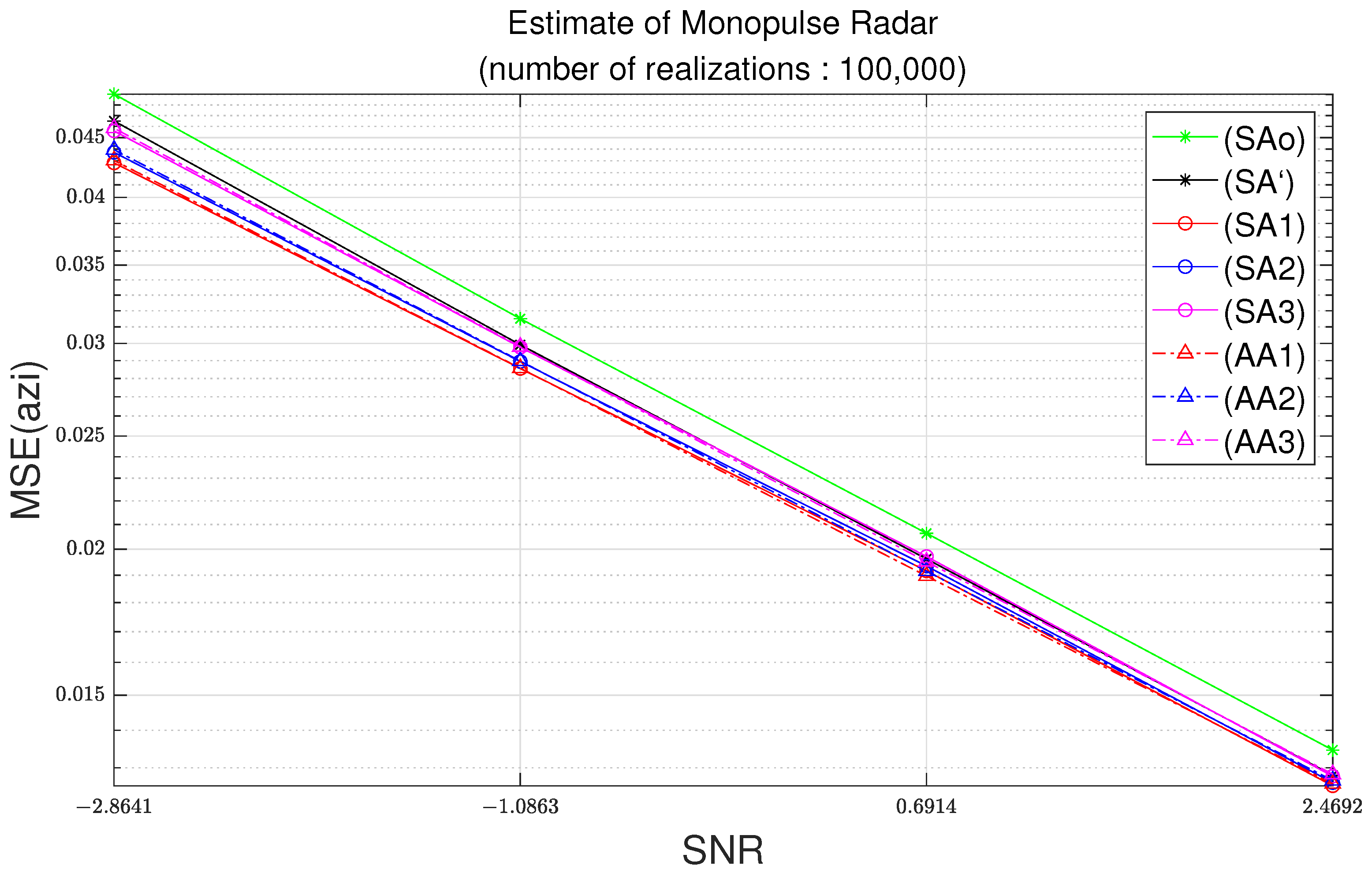
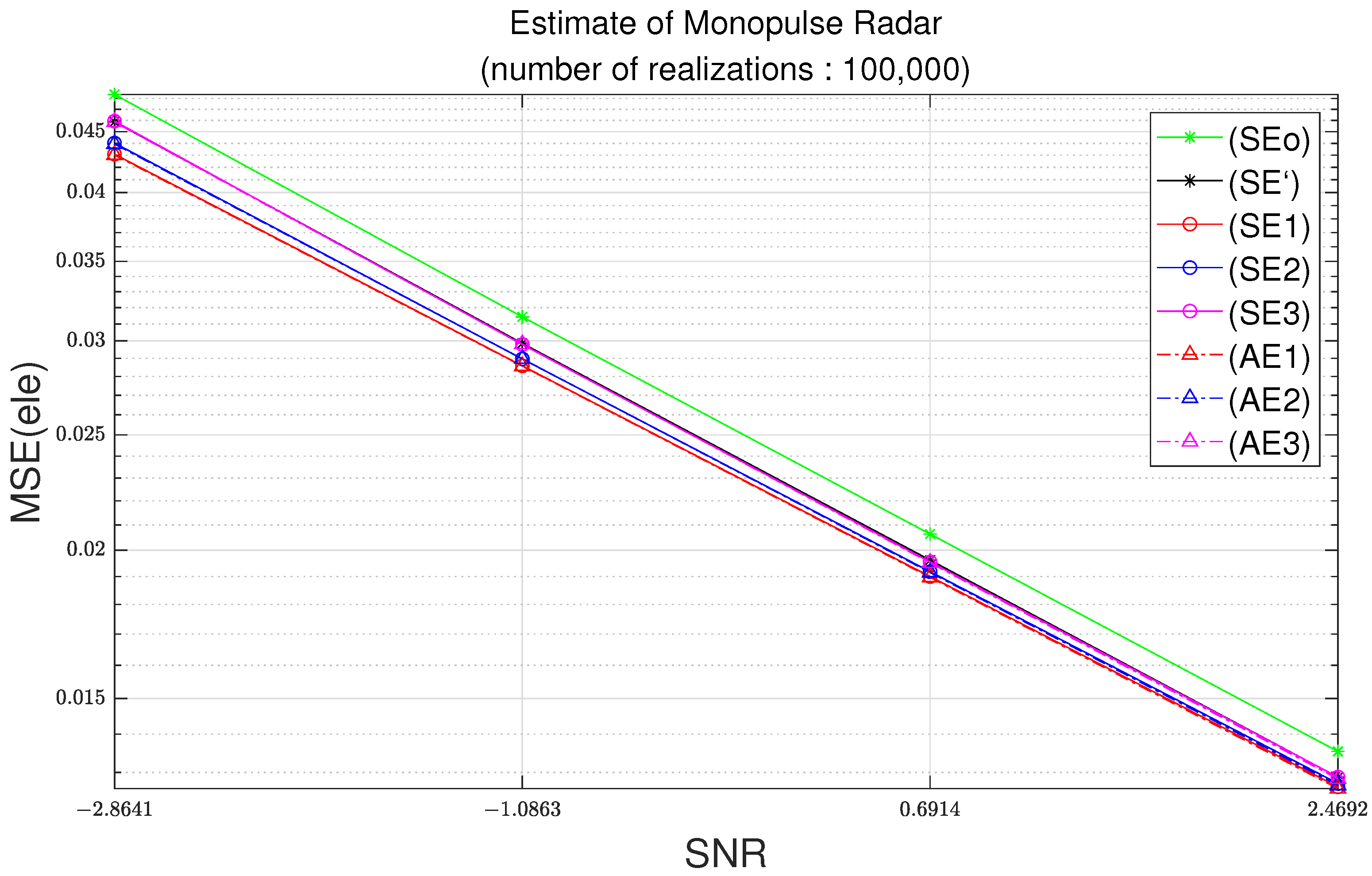
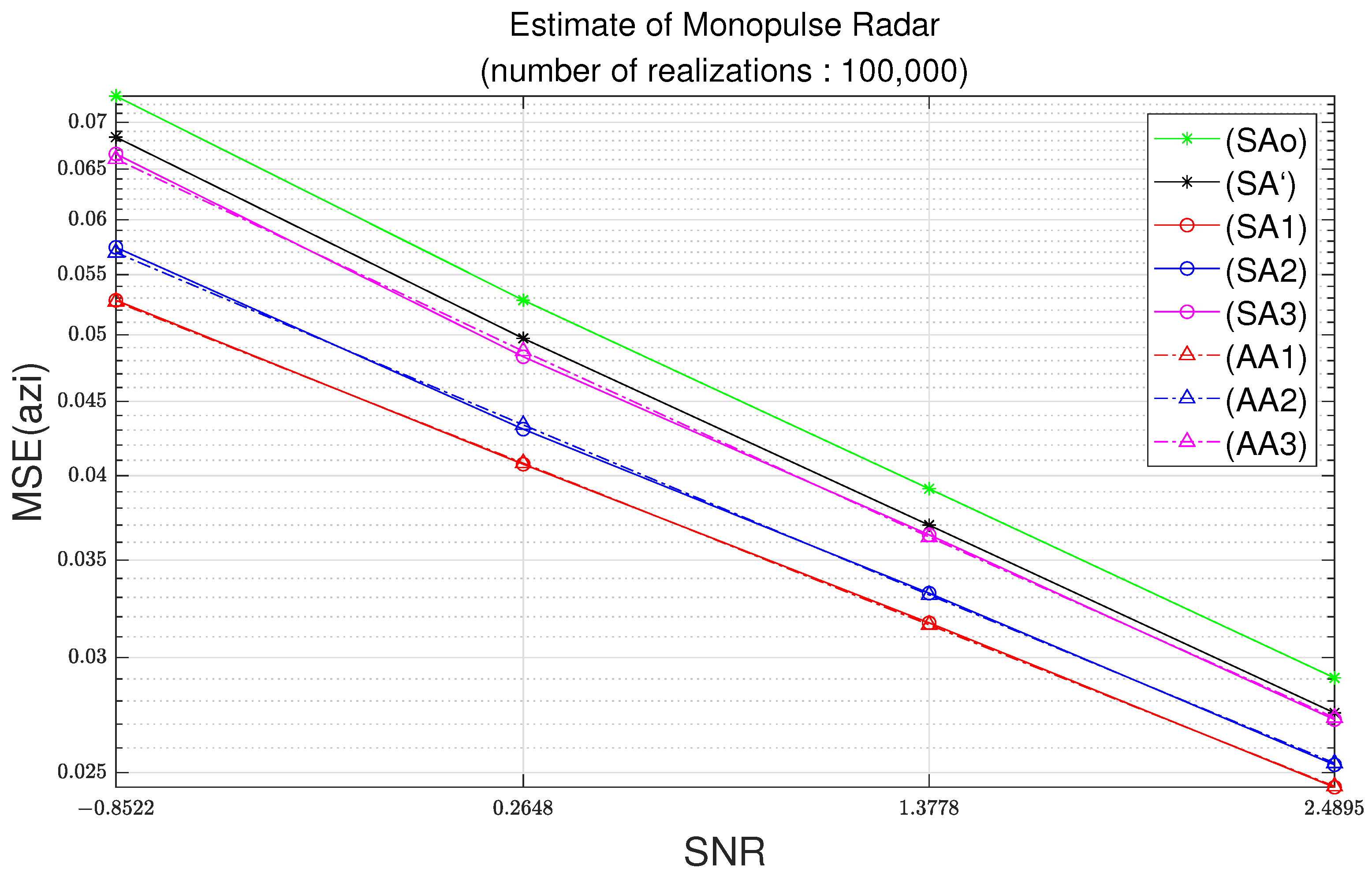
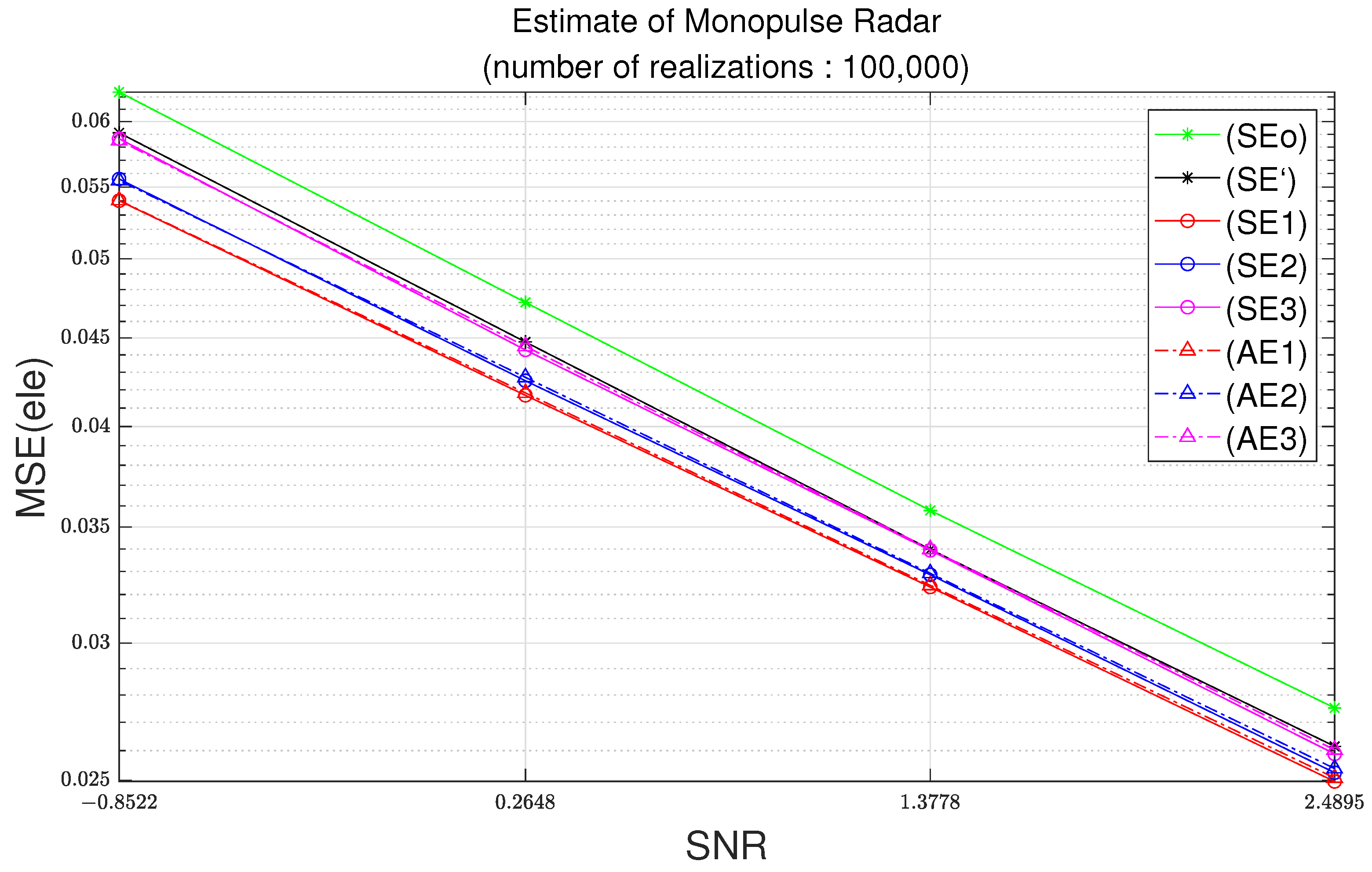
Figure 5 and Figure 6 illustrate the MSEs with respect to the signal-to-noise ratio (SNR) at 100,000 simulation trials. As the standard deviation of noise increases, the noise level increases. Therefore, the SNR decreases. The results in Figure 3 and Figure 4 illustrates the MSE with respect to the standard deviation of noise. On the other hand, the results in Figure 3 and Figure 4 illustrate the MSE with respect to the SNR.
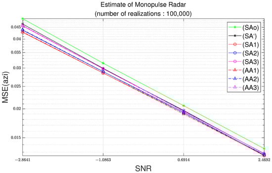
Figure 5.
Azimuth MSE as function of SNR with parameters of Table 2 and 100,000 realizations.
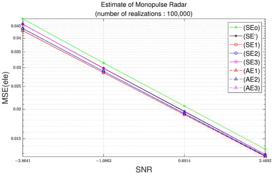
Figure 6.
Elevation MSE as function of SNR with parameters of Table 2 and 100,000 realizations.
3.2. Test 2: Simulation MSEs and Analytic MSEs
The parameters used in Test 2 changed only the standard deviations of noise from the parameters used in Test 1. It is assumed that the standard deviations of noise received in the A and D beams in Test 2 are approximately twice the standard deviations of noise used in Test 1, and the standard deviations of noise received in the B and C beams are low-magnitude noises. This test simulates a case in which noise strongly influences only A and D received beams for some reason. In Table 3, the parameters used in Test 2 are assumed to be as follows:
Table 3.
Parameters for Test 2.
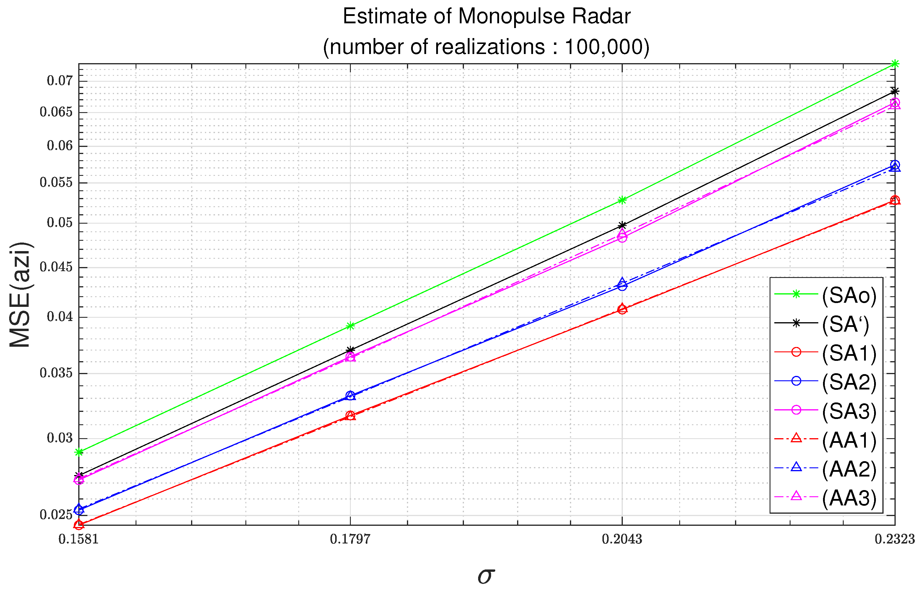
The overall results of Test 2 are similar to those shown in Test 1. However, in Figure 7, Figure 8, Figure 9 and Figure 10, the differences between the results of analytic MSEs based on third-order Taylor approximation and the results of analytic MSEs based on second-order Taylor approximation are increased. In particular, these results appear larger in the azimuth. In Test 2, it can be seen that (AA3) and (AE3) are almost close to (SA’) and (SE’), respectively. However, compared with Test 1, it can be seen that the results of (AA2) and (AE2) are farther away from (SA’) and (SE’). Similarly, it can be seen that the results of (AA1) and (AE1) are also farther away from (SA’) and (SE’) when compared with Test 1. These results show that analytic MSEs based on third-order Taylor approximation respond better to various noise environments than analytic MSEs based on first and second-order Taylor approximation.
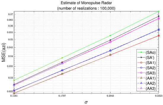
Figure 7.
Azimuth MSE as function of standard deviation with parameters of Table 3 and 100,000 realizations.
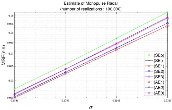
Figure 8.
Elevation MSE as function of standard deviation with parameters of Table 3 and 100,000 realizations.
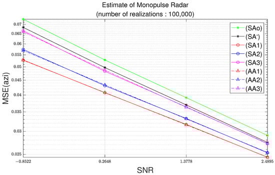
Figure 9.
Azimuth MSE as function of SNR with parameters of Table 2 and 100,000 realizations.
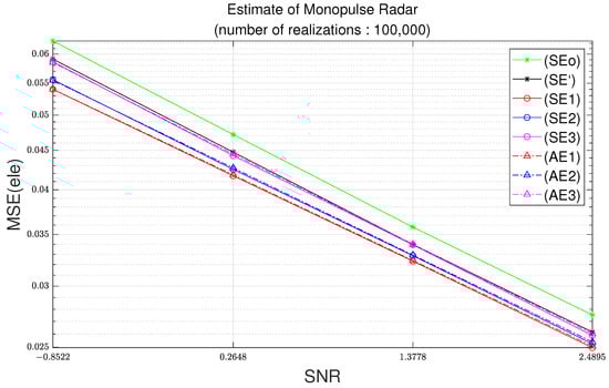
Figure 10.
Elevation MSE as function of SNR with parameters of Table 2 and 100,000 realizations.
In Figure 9, for a difference of the azimuth MSE of 0.015, the standard deviation is the square root of 0.015, which is equal to 0.12 radians; note that 0.12 radians corresponds to 7.01 degrees. In Figure 10, for the difference of elevation MSE of 0.005, the standard deviation should be the square root of 0.015, which is equal to 0.070 radians; note that 0.070 radians corresponds to 4.05 degrees. Note that the azimuth difference of 7.01 degrees and the elevation difference of 4.05 degrees can have a great influence on the tracking algorithm.
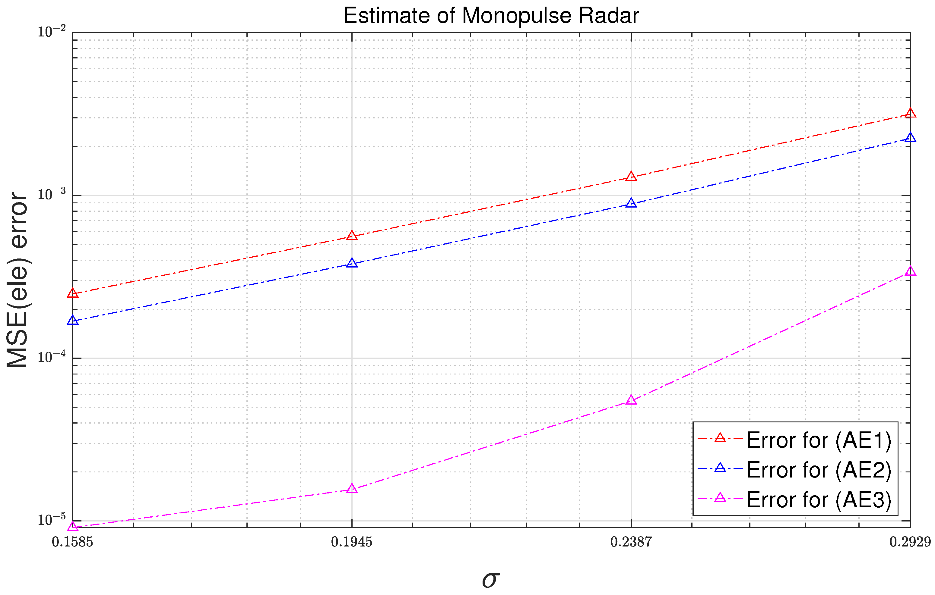
3.3. Performance of Analytic MSEs Based on Third-Order Taylor Approximation
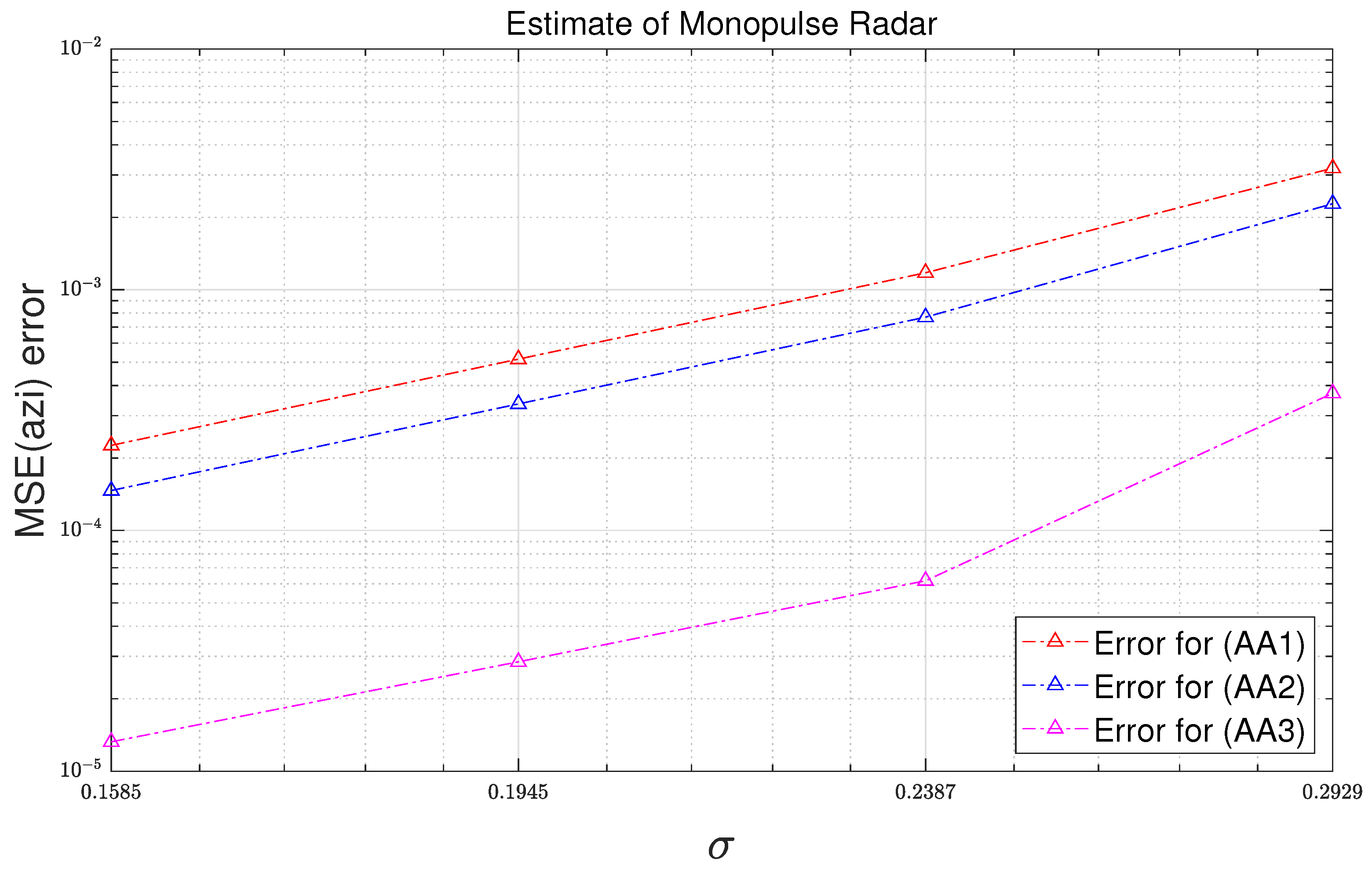
The MSE error results used in this subsection are calculated based on the results of Test 1. Figure 11 and Figure 12 illustrate the MSE errors of analytic MSE based on third-order Taylor approximation and analytic MSEs based on first-order and second-order Taylor approximation. Table 4 tabulates what the legends in Figure 11 and Figure 12 represent. The MSE errors of (AA1), (AA2), and (AA3) are obtained with reference to (SA’), and the MSE errors of (AE1), (AE2), and (AE3) are obtained with reference to (SE’). MSEs refer to the difference between the results of simulation MSEs based on (14) and (15) and the results of the analytic MSEs. In Figure 11 and Figure 12, it can be seen that the errors of the analytic MSEs based on the third-order Taylor approximation are smaller than the errors of the analytic MSEs based on the first-order and second-order Taylor approximations.
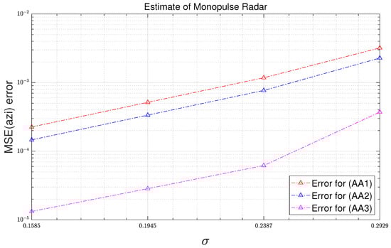
Figure 11.
Azimuth MSE errors of analytic MSE as function of standard deviation.
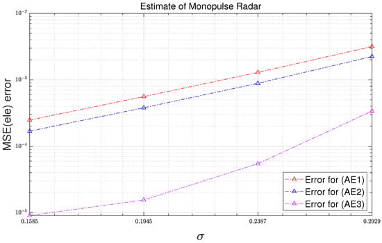
Figure 12.
Elevation MSE errors of analytic MSE as function of standard deviation.
Table 4.
MSE error expression.
Table 5 tabulates the MSE error reduction rate of “Analytic MSE (approx = 3)” compared to “Analytic MSE (approx = 2)”. The results in Table 5 shows that the error of the analytic MSE based on second-order Taylor approximation is reduced by 89.5% by using the analytic MSE based on third-order Taylor approximation.
Table 5.
MSE error reduction rate of “Analytic MSE (approx = 3)”.
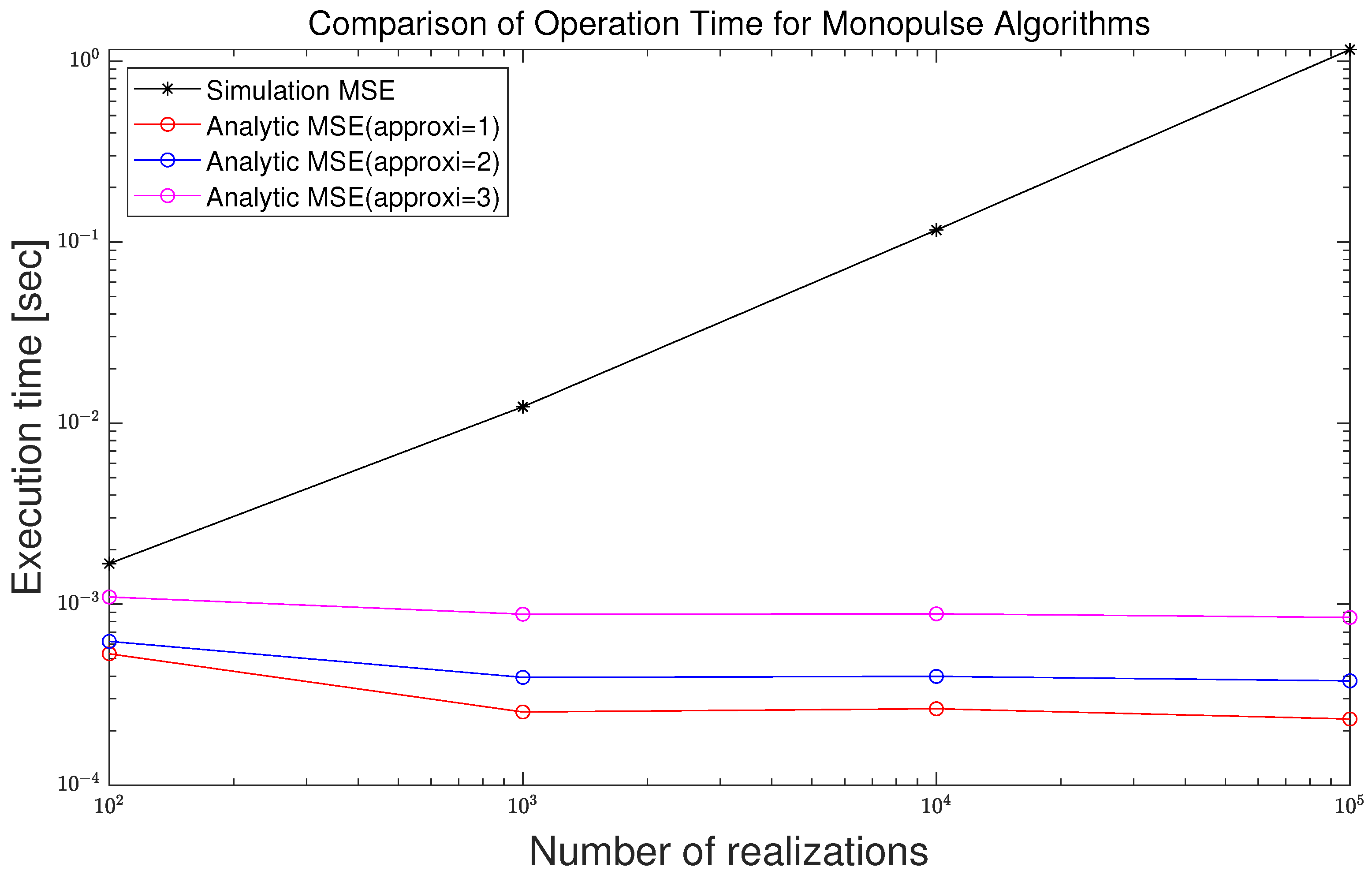
The computational complexities of the analytic approach and that of the Monte-Carlo simulation based approach are illustrated in Figure 13. The x-axis and y-axis scales of the graph are set to a log scale, and the number of simulation realizations is set to increase by an exponent of 10. In addition, operation times for all standard deviations performed in the simulation are included. “Simulation MSE” is the MSE operation time using the Monte-Carlo method based on the Taylor approximation angle estimation (A14) and (A15). The linear increase in the MSE operation time is because both the x-axis and y-axis are in log scale.
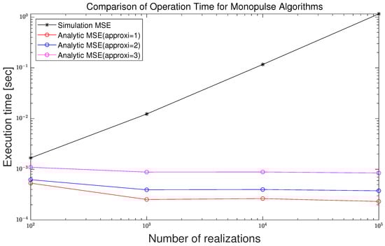
Figure 13.
Comparison of execution time as a function of the number of realizations for the simulated and analytical MSEs.
In Figure 13, the results of legend “Analytic MSE (approx = 1)”, “Analytic MSE (approx = 2)”, and “Analytic MSE (approx = 3)” are shown in order from the bottom. As shown in the results, the result with legend “Analytic MSE (approx = 1)” applying the first-order Taylor approximation is the fastest, and the result with legend “Analytic MSE (approx = 3)” applying the third-order Taylor approximation is the slowest. The operation time for the analytic approach is not dependent on the number of the realizations since the analytic MSE is not obtained from the Monte-Carlo simulation. In addition, the results of the analytic approach are much smaller than those of the simulation-based approach. The difference in the computational complexity becomes evident as the number of realizations increases.
In Table 6, the computational performance for several numbers of realizations is tabulated. In Table 6a, the operation times for computations of MSEs are measured for each method. In Table 6b, the ratios between the operation times of the simulation MSE and the operation times of analytic MSEs are summarized. From the results, the operation time of the simulation-based MSE with 10,000 realizations is 136 times as long as that of the analytically-derived MSE. In addition, from the results, the operation time of the simulation-based MSE with 100,000 realizations is 1355 times as long as that of the analytically-derived MSE.
Table 6.
Comparison of operation time.
4. Discussion
The estimation of various parameters of radar targets is affected by various noises. The types of noise include cosmic noise and thermal noise. There are also amplitude irregularities due to interference from external sources and propagation effects. The most significant of these is the thermal noise that occurs inside the receiver [7].
In this work, performance analysis is conducted for several noises without being limited to a specific noise. Therefore, the experiment is conducted using various standard deviations of the noise variables, and in most cases, the MSE of the estimated angle is calculated. When the standard deviation of the noise variable is known, the MSE can be calculated accurately and efficiently by using the analytic MSE based on the third-order Taylor approximation.
However, there are limits to this work. First, the proposed method only considers the case where the beam pattern is a specific Gaussian pattern. Therefore, this cannot be applied to a case with a beam pattern other than Gaussian. Next, we considered only the specific case where the noises in the incident signal are not correlated with each other. This makes the noise used in the MSE calculation limited. Finally, the MSE of the proposed method with the third-order Taylor expansion is slightly different from that of the original monopulse algorithm without approximation.
5. Conclusions
In this study, in order to judge the reliability of the ACM’s angle estimation ability in an environment where various noises are given, we focus on accurately calculating the MSE. Therefore, we propose an analytical MSE based on the third-order Taylor approximation with improved accuracy in terms of the MSE. The analytic MSE method based on the third-order Taylor approximation can efficiently and accurately calculate the MSE of an angle estimate quantitatively once the variance of additive noise is given.
The MSEs associated with the third-order Taylor expansion are much smaller than those with the second-order Taylor expansion. In addition, the computational complexity of the analytically-derived MSE is much smaller than that of the Monte-Carlo simulation-based MSE.
In the Monte-Carlo simulation based approach, for the MSEs to be reliable, the number of realizations should be large enough, which results in the increase in the computational complexity. From Figure 2, for the simulation-based MSE to be reliable, the number of realizations should be greater than 10,000. When comparing the analytical MSE through the third-order Taylor approximation and the MSE through the Monte-Carlo method, it can be seen that the computational amount of the analytical MSE method is less than that of the Monte-Carlo method. In Table 6, the operation time of the analytically-derived MSE is 0.76% of that of the simulation-based MSE from 10,000 realizations, and the operation time of the analytically-derived MSE is 0.07% of that of the simulation-based MSE from 100,000 realizations. This means that the operation speed is 1355 times faster. Therefore, the proposed analytic approach is much better than the Monte-Calro simulation-based approach in terms of the computational complexity.
In addition, by adopting the third-order Taylor expansion, the estimation accuracy is improved in comparison with the approaches based on the first-order Taylor expansion and the second-order Taylor expansion. In Tests 1 and 2, analytic MSEs based on the third-order Taylor approximation almost overlap with the simulation MSE results of estimation equations to which gain approximations are applied. In particular, in Test 2, it can be seen that analytic MSEs based on third-order Taylor approximation respond better to various noise environments than analytic MSEs based on the first and second-order Taylor approximations proposed in a previous study. In Table 5, it can be seen that the error of the analytic MSE based on the third-order Taylor approximation is reduced by approximately 89.5% compared to the error of the analytic MSE based on the second-order Taylor approximation. However, the computational complexity of the third-order Taylor expansion is slightly greater than that of the second-order Taylor expansion.
As mentioned in the Discussion, in Figure 3 and Figure 5, there is always a certain difference between the result of (SAo) and the result of (SA3). The same observations are also found in Figure 4 and Figure 6, which illustrates the elevation MSEs. Obtaining analytic expressions for the results with legend (SAo) and the results with legend (SEo) will be a future research topic. In addition, analyzing the estimated angle MSE of the ACM radar considering the correlated noise will also be a future research topic.
Author Contributions
H.-W.H. created the Matlab simulation and wrote the initial draft. J.-H.L. and H.-W.H. derived the mathematical formulation of the proposed scheme. In addition, J.-H.L. checked the numerical results and corrected the manuscript. All authors have read and agreed to the published version of the manuscript.
Funding
The authors gratefully acknowledge the support from Electronic Warfare Research Center at Gwangju Institute of Science and Technology (GIST), originally funded by Defense Acquisition Program Administration (DAPA) and Agency for Defense Development (ADD).
Conflicts of Interest
The authors declare no conflict of interest.
Appendix A. Angle Estimation Equations Using Taylor Approximation
In this Appendix, the angle estimation equations are derived in detail using the Taylor series expansion. First, expansion is performed for the azimuth.
Random variables for noise are set as follows:
The third-order Taylor series expansion for four variables is [15]
Each Taylor series term can be substituted with auxiliary variables as follows:
In Table A1, the coefficients of the first Taylor series and second Taylor series are tabulated [12].
Table A1.
First-order and second-order Taylor coefficients.
In Table A2, the coefficients of the third-order Taylor series are tabulated.
Table A2.
Third-order Taylor coefficients.
The expansions of the Taylor coefficients for , , and are given in Appendix C.
Expanding in (A3) results in:
Expanding in (A3) results in
The elevation estimation equation based on Taylor approximation can also be obtained in the same way as the azimuth. The signs of and of the elevation estimation Equation (15) are opposite to the signs of and of the azimuth estimation Equation (14). Therefore, the elevation estimation equation based on Taylor approximation can be obtained by exchanging the positions of and in (A4)–(A6) related to the azimuth:
The simple forms of the first-order Taylor approximation equation for angle estimation are given by
where and are first-order Taylor series terms of azimuth and elevation, respectively.
The simple forms of the second-order Taylor approximation equation for angle estimation are given by
where and are second-order Taylor series terms of azimuth and elevation, respectively.
In order to significantly improve the accuracy of the estimated angles shown through the first-order and second-order Taylor approximations, the third-order Taylor approximation is performed for estimated angles:
where and are third-order Taylor series terms of azimuth and elevation, respectively.
Appendix B. Explicit Expression of the MSEs Based on the Third-Order Taylor Approximation
In (A4), terms with a variable with a maximum power of one can be substituted with auxiliary variable () as follows:
Therefore, can be simplified as follows:
As in (A16), terms with a variable with a maximum power of one are substituted with , and terms with a variable with a maximum power of two are substituted with :
Therefore, can be simplified as follows:
As in (A18), terms with a variable with a maximum power of one are substituted with , terms with a variable with a maximum power of two are substituted with , and terms with a variable with a maximum power of three are substituted with . It can be substituted with auxiliary variables as follows:
Similarly, can be simplified as follows:
The MSE expansion of the angle estimation equation of the first-order Taylor approximation and the second-order Taylor approximation can be found in [12]. From (A10), the MSE of the azimuth for the first-order Taylor approximation can be written as
Using (A17), it can be summarized as follows:
Similarly, from (A12), the MSE of the azimuth for the second-order Taylor approximation can be written as
Using (A19), it can be summarized as follows:
When in (A25) is expanded using (A18), there are variables with odd powers in all terms. Referring to (A58) and (A59), it can be seen that if a variable with an odd power exists in a term, the term becomes zero. Therefore, is zero.
Similarly, for the same reason as mentioned above, in (A26) is zero:
Using (A23), (A25) and (A26), the analytic MSE of the azimuth based on the second-order Taylor approximation is summarized as follows:
Equation (A28) is an equation that applies the MSE to the azimuth estimation equation based on third-order Taylor expansion in (A14):
Using (A21), expands as follows:
For the same reason as mentioned above, and in (A29) is zero.
In (A30), when is expanded, is zero because all terms have odd power variables.
For the same reason as mentioned above, in (A31) also becomes zero.
The analytic MSE of the azimuth based on the third-order Taylor approximation proposed in this paper is summarized as follows:
The analytic MSE of elevation can also be derived in the same manner as that of the azimuth.
Equations (A33) and (A34) are analytic MSEs based on first-order Taylor approximation:
where is terms with the maximum power of one at the estimated elevation of the first-order Taylor series terms.
Equations (A35) and (A36) are analytic MSEs based on second-order Taylor approximation:
where and are terms with a maximum power of one and a term with a maximum power of two at the estimated elevation of the second-order Taylor series terms, respectively.
Equations (A37) and (A38) are analytic MSEs based on third-order Taylor approximation:
where , , and are terms with a maximum power of one, terms with a maximum power of two, and terms with a maximum power of three in the estimated elevation of the third-order Taylor series terms, respectively.
In order to expand (A33)–(A38) into a complete form, it is necessary to fully expand the terms consisting of A, B, and C. Referring to (A57)–(A59), when (A16), (A18) and (A20) are squared and the expectation operations are applied to the squaring result, terms consisting of even power variables remain. Therefore, using (A57)–(A59), (A39)–(A44) can be obtained as functions of standard deviations and Taylor coefficients:
Similarly, (A45)–(A47) can be obtained in the same way. Since the expectation operations are applied to the expanded expressions, terms with odd power variables become zeros, and only terms with even power variables remain:
Appendix C. Characteristics of Noise Random Variables and Derivation of Taylor’s Coefficients
It is assumed that the noises of the signal received by the ACM radar are Gaussian random variables and have the following parameters:
It is also assumed that the noises are not correlated with each other:
Equations (A69)–(A71) correspond to the coefficients of the first-order, second-order, and third-order Taylor approximation equations, respectively. In (14), since the sign of and the sign of are the same, and the sign of and the sign of are the same, it can be expressed as follows [12]:
where is the azimuth () true angle or elevation () true angle. Since these coefficients are applied equally for the azimuth and elevation, can be expressed by replacing .
References
- Rhodes, D.R. Introduction to Monopulse; Artech House: Norfolk County, MA, USA, 1980. [Google Scholar]
- Leonov, A.I.; Fomichev, K.I. Monopulse Radar; Artech House: Norfolk County, MA, USA, 1986. [Google Scholar]
- Sherman, S.M.; Barton, D.K. Monopulse Principles and Techniques; Artech House: Norfolk County, MA, USA, 1984. [Google Scholar]
- Hofstetter, E.; DeLong, D. Detection and parameter estimation in an amplitude-comparison monopulse radar. IEEE Trans. Inf. Theory 1969, 15, 22–30. [Google Scholar] [CrossRef]
- Davis, R.C.; Brennan, L.E.; Reed, L.S. Angle estimation with adaptive arrays in external noise fields. IEEE TRansactions Aerosp. Electron. Syst. 1976, AES-12, 179–186. [Google Scholar] [CrossRef]
- Zheng, Y.; Tseng, S.-M.; Yu, K.-B. Closed-form four-channel monopulse two-target resolution. IEEE Trans. Aerosp. Electron. Syst. 2003, 39, 1083–1089. [Google Scholar] [CrossRef]
- Richards, M.A.; Scheer, J.A.; Holm, W.A. Principles of Modern Radar Basic Principles; SciTech Publishing Inc.: Raleigh, NC, USA, 2008; Volume 1. [Google Scholar]
- Jacovitti, G. Performance Analysis of Monopulse Receivers for Secondary Surveillance Radar. IEEE Trans. Aerosp. Electron. Syst. 1983, AES-19, 884–897. [Google Scholar] [CrossRef]
- Chen, L.; Sheng, W. Performance analysis for angle measurement of monopulse radar with non-consistent amplitude-phase features. In Proceedings of the IEEE 2010 International Conference on Microwave and Millimeter Wave Technology, Chengdu, China, 8–11 May 2010. [Google Scholar]
- Mosca, E. Angle estimation in amplitude comparison monopulse systems. IEEE Trans. Aerosp. Electron. Syst. 1969, AES-5, 205–212. [Google Scholar] [CrossRef]
- Kim, M.J.; Hong, D.S.; Park, S.S. A study on the amplitude comparison monopulse algorithm. Appl. Sci. 2020, 10, 3966. [Google Scholar] [CrossRef]
- An, D.J.; Lee, J.H. Performance analysis of amplitude comparison monopulse direction-of-arrival estimation. Appl. Sci. 2020, 10, 1246. [Google Scholar] [CrossRef] [Green Version]
- Han, Y.J.; Kim, J.W.; Park, S.R.; Noh, S.U. An investigation into the monopulse radar using tx-rx simulator in electronic warfare settings. In Proceedings of the Symposium of the Korean Institute of Communications and Information Sciences, Jeongseon, Korea, 18–20 January 2017; pp. 705–706. [Google Scholar]
- Park, S.R.; Nam, I.K.; Noh, S.U. Modeling and simulation for the investigation of radar responses to electronic attacks in electronic warfare environments. Secur. Commun. Netw. 2018, 2018, 3580536. [Google Scholar] [CrossRef]
- Taylor Series. Encyclopedia of Mathematics. Available online: https://encyclopediaofmath.org/wiki/Taylor_series (accessed on 30 April 2021).
- Normal distribution. Available online: https://en.wikipedia.org/wiki/Normal_distribution (accessed on 30 April 2021).
Publisher’s Note: MDPI stays neutral with regard to jurisdictional claims in published maps and institutional affiliations. |
© 2021 by the authors. Licensee MDPI, Basel, Switzerland. This article is an open access article distributed under the terms and conditions of the Creative Commons Attribution (CC BY) license (https://creativecommons.org/licenses/by/4.0/).