Review

The Decreasing Hazard Rate Phenomenon: A Review of Different Models, with a Discussion of the Rationale behind Their Choice

1
Department of Industrial Engineering, University of Naples Federico II, 80125 Naples, Italy
2
Department of Electrical, Electronic and Information Engineering, University of Bologna, 40136 Bologna, Italy
*
Author to whom correspondence should be addressed.
Electronics 2021, 10(20), 2553; https://doi.org/10.3390/electronics10202553
Submission received: 8 September 2021 / Revised: 6 October 2021 / Accepted: 12 October 2021 / Published: 19 October 2021
(This article belongs to the Section Industrial Electronics)

Abstract

:
It is well known that, especially in the field of electronic components reliability studies and applications, the Exponential reliability model is by far the most adopted, although the data fostering it are few. This appears to be due partly to its simplicity (also in view of estimation, since it is characterized by a unique parameter), and partly because most components seem to be well represented, at least in their “useful life” time interval, by the Exponential model. This adoption is basically due to its peculiar “memory-less” property, i.e., the fact that such model possesses a constant hazard rate function, meaning that stochastic “accidents” cause the failure of the component, independently of its service time. This theoretical reason behind the choice of the Exponential model is largely prevailing over the classical statistical “goodness of fit” tests, since the high-reliability values attained by such devices does not allow the availability of an adequate number of lifetime values to be observed and analyzed in a statistical data analysis procedure. A second model also widely adopted is the Weibull model, especially if characterized by a shape parameter greater than unity, so implying an increasing hazard rate function. However, there are many cases—which can be also justified on a theoretical basis, as reviewed in this paper—in which a decreasing hazard rate function (at least for relatively large mission times) may be the best suited to describe the true model behind a given failure mechanism. The afore-mentioned theoretical basis of these apparently peculiar models is the main core of the present review article, whose aim also includes the illustration of the basic features of the main reliability models featuring an hazard rate function diminishing with time. The paper also discusses, resorting to graphical and numerical case-studies relevant to both field and simulated data, the consequences of mistaken model identification in terms of the hazard rate function behaviour, which may imply wrong maintenance actions.

1. Introduction

Reliability is more and more a key problem in engineering, especially in the field of electronics, as witnessed by a recent special issue on this topic, focused on Power electronic devices reliability [1,2,3,4,5,6,7,8,9,10,11,12,13,14,15,16]. Nowadays, indeed, these are becoming more and more critical devices, since—as highlighted in [16]—ower electronics plays a crucial role in renewable energy systems, lighting, electric mobility, and other systems that enable sustainable development.
It is well known that modern reliability theory, as witnessed by a growing series of authoritative books on the topic [17,18,19,20,21,22,23,24,25,26,27,28,29,30,31,32,33,34,35,36,37,38,39,40,41,42,43,44], is based upon consolidated theoretical probabilistic models [45] which find their justification in ad hoc statistical methods: these are however becoming difficult to apply, due to typical scarcity of failure data availability, as a consequence of the high and ever increasing reliability degree attained by modern components. Another aspect which undermines classical or traditional statistical methods is the randomness or unpredictability of environmental conditions in which the devices will operate, often very different from the laboratory test conditions. For instance, as discussed in [1] regarding again power electronics devices, these are expected to operate under challenging environmental conditions (e.g., high altitudes in more electric aircrafts or high temperatures on photovoltaic installations), compromising the effectiveness of traditional approaches, typically based on historical failure data and past observed scenarios. In fact, the rapid evolution of power electronic technologies and the ever more challenging operating frameworks pose severe limitations on the trustworthiness of available reliability data, as they are typically related to incoherent operating conditions [1,2,3,4].
Thus, new methods have been developed such that the reliability model identification and estimation of most of the modern components, as those above exemplified, may be better achieved, instead that using limited lifetime data, by the knowledge of the degradation mechanisms, and the consequent assessment of the wear process affecting the device’s lifetime [46,47,48,49,50,51,52,53,54,55,56,57,58,59,60,61,62,63,64,65,66,67,68,69,70,71,72,73]. Such methods have developed the results initiated in 1973 by the seminal paper by Esary and Marshall [46] on shock models and wear processes, and successive basic papers as [47,48,49,50,51,52,53], and ultimately have taken advantage of a large series of theoretical results on the relationship between the theory of stochastic processes (or random functions of time) and reliability [74,75,76,77,78,79,80,81,82,83,84].
On the other hand, as discussed in [1], power electronic devices reliability is affected by thermal, electrical and mechanical stresses, and in the presence of such stresses it can be assessed through consolidated, traditional methods and techniques. Such methods, which often allow an efficient estimation of the state of the health of the device, can constitute a powerful basis for building the so-called “indirect” or “physical” reliability models assessment [72,73,74,75,76], even in the absence of many data. This is the basic purpose of the present review, aiming in particular at discussing the foundations of a particular sub-class of the Reliability models (RM), i.e., those possessing a decreasing hazard rate function (HRF)—at least for relatively large mission times. The definition of decreasing HRF is recalled afterwards, and it will be shown that the discussion of decreasing HRF may constitute a great help into a deeper understanding of the rationale behind choice of a given RM.
Very often, indeed, the largely most widespread RM, i.e., the Exponential model (the unique model possessing a constant HRF) and the Weibull model (especially if characterized by a shape parameter greater than unity, so implying an increasing HRF), are adopted without any reason apart from—in practice—their simplicity, also in view of consolidated estimation procedure [33].
The Exponential model in particular is sometimes justified on a statistical basis, i.e., by conducting adequate statistical tests on the available failure data, but it is mostly motivated relying on the theoretical basis that such model is the only one characterized by a constant hazard rate function, meaning that stochastic “accidents” cause the failure of the component, independently of its service time. This second, theoretical reason, behind the choice of the Exponential model is largely the prevailing one nowadays, since the high-reliability values attained by such devices does not allow the availability of an adequate number of lifetime values to be observed and analyzed in a statistical data analysis procedure.
As above hinted at, this is the fundamental reason behind the development of “indirect” or “physical” reliability models assessment, based on the study of wear or degradation processes acting on the device. A peculiar consequence of such kind of analysis, surprisingly rarely emphasized in literature, is that such models imply a fact that is maybe contrary to intuition, namely a hazard rate function which is decreasing over time—at least for relatively large mission times. More precisely, most of such theoretical models imply an HRF which is, alternatively:
-
always decreasing in time (the class of such models is denoted as “decreasing hazard rate”, DHR);
-
first increasing, then decreasing in time (the class of such models is denoted as “first increasing, then decreasing hazard rate”, IDHR).
Sometimes, the IDHR class is also denoted as “unimodal HRF“, since in this class the HRF possesses a unique maximum at a certain time instant t*, while it is increasing from t = 0 to t*, then decreasing after t*. Such instant t* is also denoted, for obvious reasons, a “change point” of the HRF.
The previously mentioned characteristics may be connected to the features of wear or degradation processes. Moreover, new insights have been gained on the theory from extensive studies on maintenance strategies [85,86,87,88,89,90,91,92,93], since they are in some way related to the HRF behavior, as will be clear when we introduce the meaning of the HRF later.
Indeed, in view of the purpose of the present paper, in the following a brief review is presented for illustrating the basic relations existing among the fundamental Reliability measures, the most important of which are:
  • the Reliability function (RF);
  • the above introduced hazard rate function (HRF);
  • the Mean Time to Failure (MTTF);
  • the “residual reliability function” (RRF).
More refined details on such relations can be found in the above cited references [17,18,19,20,21,22,23,24,25,26,27,28,29,30,31,32,33,34,35,36,37,38,39,40,41,42,43,44,45].
Indicating as T the non-negative RV “time to failure”, or “lifetime” (LT), of the device and as F(t) its cumulative distribution function (CDF), the RF can be stated as here below:
R(t) = P(T > t) = 1 − F(t)
being P(A) the probability of the generic random event A. The above RF is sometimes denoted also as “survival function” in literature. The RV T is typically assumed, of course being a time variable, as a continuous RV, distributed according to a probability density function (PDF) f(t) such that:
f(t) = dF/dt = −dR/dt
and
R t = t f u d u
It is remarked that the RF R(t) represents the probability that the component works satisfactorily over all the period (0,t). MTTF indicates the expected LT and can be obtained, provided that the integral exists, by:
E T = 0 R t d t
As pointed out in the above cited references [17,18,19,20,21,22,23,24,25,26,27,28,29,30,31,32,33,34,35,36,37,38,39,40,41,42,43,44,45], the Reliability theory can be viewed mathematically as an applied probability theory focusing on positive RVs. Nevertheless, it features parameters and functions established precisely to illustrate time-related RVs (especially–but non exclusively–Lifetimes). In practice these parameters and functions miss counterparts in different fields of probability theory.
Among them, the HRF is the most widely employed to illustrate component aging. Contrary to the CDF and the RF—both related to a time period, see above—the HRF h(s) is related to the instant s ≥ 0, to be meant as the component “age”. Indeed, it is also known as the “instantaneous failure rate” at a certain time instant. From a formal viewpoint, if f(t) is the PDF of LT, T, the HRF is defined as:
h t = f t R t = d d t log R t
at each time t ≥ 0 for which R(t) ≠ 0.
An equivalent definition, which also explains the origin of its name, as well as its meaning, is the following:
h x = lim Δ x 0 + P x < T x x + Δ x ( T > x ) Δ x = l i m Δ x 0 + F x + Δ x F x Δ x   R x
Therefore, for Δx→0+, the quantity h(xx is equal to the conditional probability that the failure takes place within the interval (x, x + Δx), provided that the component has reached an age x (i.e., it did not fail—or survived—until x); namely h(x)Dx can be viewed as the instantaneous failure (conditional) probability of a component having age x.
Once imposed the trivial condition R(0+) = 1, an integral relationship can be derived that lets the RF, R(t), be explained as a function of the instantaneous HRF:
R t = e x p 0 t h ξ d ξ ,   t > 0
As a consequence, by fixing either the PDF, or the RF or the HRF of a reliability model, the model itself is completely defined, as every one of such three functions can provide straightforwardly the other two: for instance, from (7) h(t)—whose functional expression can be deduced in some cases relying on its physical grounds—provides directly the RF. Thereafter, the PDF can be obtained via the well-known equation:
f(t) = h(t) R(t)
In a similar way, the MTTF, CDF, etc. can be simply attained, too.
As a further illustration, in such a way the 2-parameter Weibull model (the most popular one when investigating reliability in engineering applications) can be easily derived, too, which features the following expressions for the dependency of RF, HRF, PDF vs. time t > 0:
R(t) = exp(−αtβ)
h(t) = αβtβ−1
f(t) = h(t) R(t) = αβtβ−1 exp(−αtβ)
where positive-defined quantities α and β are the scale and shape parameters respectively.
In the sequel, the Weibull model is indicated as W(α,β) (an alternative form is introduced in Section 6 (Equation (54)). When β = 1, the Weibull model reduces to the above-mentioned Exponential reliability model. It is an increasing hazard rate (IHR) model when β = 1, and a decreasing hazard rate model when β < 1. As illustrated in many textbooks [17,18,19,20,21,22,23,24,25,26,27,28,29,30,31,32,33,34,35,36,37,38,39,40,41,42,43,44,45], the time trend of the HRF may suggest the reasons behind a failure: a decreasing HRF indicates “infant mortality” or “wear-in”: namely, poorly-manufactured devices broke soon due to brittleness, flaws, etc.; on the whole the HRF drops over time with the removal of failed devices from the population. A steady HRF (Exponential reliability model only, see above) indicates that the component breaks, independently of its service time, due to stochastic “accidents”. A rising HRF indicates that the component undergoes “wear-out”, thus its failure probability increases with time.
The possible behaviors of the HRF are perhaps better understood, following [73], if the “residual reliability function” (RRF) is introduced, which is a function of two time variables (s and t in the sequel) defined as follows:
R(t|s) = P{T > s + t|T > s} = R(t + s)/R(s) (t, s ≥ 0)
The above RRF, denoted as the residual reliability function for a mission time t of a component of age s, is equal to the conditional probability that, after the component has survived until age s, it will survive at least until time (s + t), i.e., its age will increase of at least t time units in addition to s. Of course the RRF shall behave as a RF vs. time t, for example it shall satisfy: R(0|s) = 1, R(∞|s) = 0, and be decreasing with t. Its behavior with age s might appear less obvious, as discussed in [73]. E.g., in principle one might guess that, as aging is expected to make all components weaker, R(t|s) drops with s, but this does not necessarily hold, as this guess neglects that the RRF is a conditional probability, and conditioning might remarkably modify our information. For instance, in some cases, the information that a component’s age has reached a value s might make engineers more confident in its “future” survival than in the case that such information is missing; therefore, the component seems to ”get stronger” with age, and the RRF may rise with s. In any case, it should be clear that (un- conditional) RF must always decrease with time: this is a basic property originating from the very definition of a RF, and has no connection with the time variation of the HRF and/or the RRF.
Instead, there is a close relationship between the HRF and the RRF behavior [17,73]: i.e., the HRF h(s) increases (decreases) with age if and only if the RRF R(t|s) decreases (increases) with age s; the HRF h(s) is constant with age s if and only if the RRF R(t|s) constant with s, what happens only—as already pointed out many times above—with the Exponential model, by far the most adopted in the field of electronics, thereby proving that such model is “memoryless”.
However, as witnessed by all well-known standards on reliability [94,95], the methodology of the Exponential reliability model has been indeed criticized in the last years [96,97]. Also to the popular “bathtub curve” of the HRF [98] has been object of very recent criticisms in an authoritative paper by Pecht in 2021 [99]. Indeed, according such model—which is based upon the above interpretation of the RRF, but also relies upon experimental evidence originated by studies on human lifetimes-implies a HRF which first decreases, then becomes approximately constant with age (the “useful life” period, characterized only by accidental failures), finally increases with time due to wear out.
Nonetheless, as can be derived from all the models which will be analyzed in the following (and which are of course not exhaustive of the class of the RM), often the HRF behaviour in time is quite the opposite of the above model. It is also noticeable that most, if not all, of such DHR or IDHR models can be deduced, as it will be shown, in the framework of adequate so-called “stress-strength” (SS) models [100,101,102,103,104,105], to be recalled in the next section.
By discussing such aging models, this review is also aimed at highlighting the rationale behind a proper and accurate selection of a reliability model for the above devices, which is a very useful approach in view of the above discussed scarce availability of lifetime values. It also discusses the consequences of mistaken model identification in terms of the HRF behaviour. Indeed, an insight into the models shows that, although some of them appear to possess similar shape of their PDF or RF, and possess very close values of the mean and the SD, or of their “central” quantiles (e.g., the median), as clearly shown in the application of the final section—their HRF may be rather (or very) different, and the same holds for their “extreme” quantiles. This is apparent when examining various couples of RM, e.g., the Weibull and the Lognormal models (as also illustrated in the numerical application), as well the Weibull and the Log-Logistic models, or the Birnbaum-Saunders and Inverse Gaussian model, and more). This theoretical aspect may have serious consequences, e.g., in terms of the maintenance actions to be taken on such devices [85].
The rest of this paper is organized as follows. Section 2 presents a brief account of the SS model and then, a list of the basic DHR and IDHR models deducible from the above SS model, to be discussed in the successive sections. Such DHR and IDHR models (Birnbaum-Saunders, Inverse Gaussian, Inverse Weibull, Log-Logistic, Lognormal model) are indeed discussed in Section 3, Section 4, Section 5, Section 6, Section 7 and Section 8. Also the Exponential model is discussed (in Section 4) for its importance, for its being at same time a DHR and IHR model, and also for illustrating a peculiar method for its deduction from an SS model.
Also, in Section 9, some DHR or IDHR models generated by mixtures of Exponential or Weibull RV are presented, in order to illustrate another completely different mechanism involved in the same above-discussed family of models. This kind of mechanism appears to be a fundamental one for electronics devices, because of the aforementioned randomness of environmental conditions in which these devices typically operate [1].
Finally, in Section 10, the aforementioned application related to real electronics lifetime data is illustrated, in order to show the possible consequences of model mis-specifications which may become very likely in the presence of a limited amount of data.

2. A Premise to the Review of the Basic DHR or IDHR Lifetime Models on the Basis of Stress-Strength Models

In the following Section 3, Section 4, Section 5, Section 6, Section 7, Section 8 and Section 9, a review of the basic DHR or IDHR lifetime models is discussed; the models are theoretically deduced by generative mechanisms originated by wear or stress processes, as explained below. For this purpose, a brief reminder of “stress-strength” (SS) models [100,101,102,103,104,105], arising from shock or wear processes is presented here, while a list of the above models, which will be illustrated in the following sections, is presented at the end of this section.
The first part of this section presents a brief account of the stress-strength model, which is probably the most straightforward method among the aforementioned “indirect reliability assessment” methods. In its simplest form, such model is introduced as a method for evaluating the reliability a device (or a system) that is subjected to an external stress, modeled by a RV X, against which the unit sets its own strength, modeled by another RV Y. So, the device survives if and only if its strength Y is greater than its stress X.
This allows to evaluate the reliability R of the unit as the probability that the unit withstands the stress:
R = P(X < Y)
Once the PDF and/or the CDF of the RV (X,Y) are known, the evaluation of the reliability R can be computed as follows
Let f(y) and F(y) be respectively the PDF and the CDF of the RV Y;
Let g(x) and G(x) be respectively the PDF the PDF and the CDF of the RV X.
Then under the hypothesis that the RV X and Y are statistically independent—the reliability R of the device is given by:
R = 0 g x P ( X < Y X = x ) d x = 0 g x 1 F x d x
In the above equations, time doesn’t appears (at least in explicit form), i.e., the PDF of X and Y are assumed as time-independent, or the mission time pre-determined, as in the particular case of the so-called “one-shot devices” (such as automobile air-bags, munitions, rockets), or electrical generation systems which, in a given mission time, must supply a constant load, and so on. Instead, in its most general form, accounting for time variation of the basic RV, the SS model regards X and/or Y as stochastic processes in time. For instance, let the stress be a wear (or degradation) process, here denoted by X(t), i.e., a stress which varies with time accumulating progressively on the device until the “threshold” y is exceeded (i.e., y is the device’s strength, which is here considered as a fixed constant for sake of illustration; the hypothesis will be relaxed afterwards). Then, the reliability of the device is expressed as a time function, i.e., as the RF R(t), as follows:
R(t) = P{X(s) < y,∀s∈(0,t)}
The failure time can be defined in such case as the first time instant in which the stress process X(t) exceeds the failure threshold y:
T = inf{s: s > 0, X(s) > y}
The above equations may be easily extended to the case in which also the strength Y is a stochastic process, Y(t).
In some cases, the analytical expression of stress X(t) and/or the strength Y(t) is known or may be expressed in terms of RV with known distributions, so—once the parameters of such RV are estimated—the distribution of lifetime T may be deduced by the stress and strength distributions.
For instance, one of the most adopted analytical expressions for stress X(t) is the one of a linear process:
X(t) = βt
in which β is a (positive) RV. This model assumes that the stress at time zero is zero: X(0) = 0, but can be easily extended to a more general linear model (X(t) = α + βt). In [21] these models are derived relying on physical grounds, providing exemplifications in addition to the ones given here. In many cases, the model in [17] may be a reasonable approximation (e.g., as obtained by the 1st term of a Taylor expansion) over some time interval, of a more complex random function. Returning to eqn. (17), in case the device’s strength, is a constant y, it is easy to deduce that the failure time T is expressed by the RV A and the threshold y as:
T = y/β
In case also the device’s strength is a RV, Y, then the failure time T is expressed by the ratio of the two RV Y and β as:
T = Y/β
Thus, as above hinted at in the general case, the distribution of lifetime T may be deduced once the stress and strength distributions are known, i.e., the distributions of the RV β and Y are known.
Another model, used for instance for lumen lifetimes [70], is the log-linear one for the stress process X(t):
X(t) = α exp(βt)
In which (α,β) are positive RV. Of course, a model such as (20) can be immediately transformed into a linear one by a logarithmic transformation (and defining of course a new threshold, Y’, as Y’ = log(Y)). This example shows that a linear process is more general than it could appear at a first sight.
Of course, there much more complex classes of wear processes, such as the “cumulative wear process”, the “Wiener process”, and more, which for brevity will be introduced when needed (in particular, the first class in Section 3, the second in Section 5).
Then, a list of the basic models deducible from an adequate SS model, that will be presented in alphabetical order in the following sections, is here presented:
As to the last point, regarding the so-called “Mixture” DHR or IDHR models, it is the last class of models presented: in Section 9, some DHR or IDHR models generated by mixtures of Exponential or Weibull RV are briefly illustrated. These mixtures represent (as above hinted at) another possible generative mechanism of such models which can assumes a great importance in the applications here considered, since the above discussed uncertainty or randomness of the environment in which the device operates can induce a certain degree oh “heterogeneity” which often produces DHR or IDHR models.
It is remarked that also the Weibull model W(α,β) of Equations (9)–(11) can be inserted among the DHR models, when the shape parameter b is less than 1; such case, however, although not to be forgotten, appears rarely (if ever) justified by an SS generative mechanism. Moreover, in most applications (except perhaps when fitting life data derived from infant mortality) as already stated, the parameter b is greater than 1 (for instance, in Section 10, an application related to lumen life data is presented, in which the above parameter is estimated as β = 7.890). It is also again remarked that the Weibull model covers the Exponential reliability model when β = 1.
Moreover, if not for its HRF behaviour (which is approximately linearly increasing), a brief mention of the Normal (or Gaussian) distribution has to be reminded. Indeed, such model is essential in statistical investigations since the distributions of various basic statistical estimators (such as the “Sample mean”) are well approximated, in view of the “Central Limit Theorem” [45], by the Gaussian probability distribution. Here, the Normal distribution will be mainly introduced, since from Section 3, in the framework of stress or wear processes. The PDF of a Normal RV with mean μ (a real number) and SD σ (a positive real number)—whose symbol is N(μ,σ), has the following expression:
f t ; μ , σ = 1 σ 2 π e x p 1 2 σ 2 t μ 2
where −∞ < t < +∞, −∞ < μ < +∞, σ > 0. The popular key features of the Normal PDF are that it is bell-shaped and symmetrical around the mean μ. The standard Normal PDF, φ(z), and CDF, Φ(z), are often used to recast the Normal PDF and CDF in terms of a Normal RV z with zero mean and unit variance. Φ(z) and φ(z) can be written, respectively as reported here below:
φ z = z 1 2 π e x p u 2 2 d u ;             φ z = d φ z d z
It is observed that, if Z is a N(μ,σ), then Z = (X − μ)/σ is a N(0,1) RV, so that: T = μ + σZ. Thus, the PDF and CDF of the N(μ,σ) Gaussian model of a RV T are expressible respectively in terms of φ(z) and Φ(z), as follows:
f t ; μ , σ = Φ t μ / σ σ ;   F t ; μ , σ = Φ t μ / σ
Obviously, the Gaussian distribution is not appropriate for the RV lifetime, as it encompasses the interval t < 0, i.e., negative times. However, it is sometimes adopted provided that μ > 3σ, but its adoption is also strongly limited by its lack of flexibility (only symmetrical, bell shaped PDF can be of course represented by this model; and also in such case a valid alterative, which does not possesses the evident drawback of a Normal model, is a Weibull model W(α,β) with β ≈ 3.6). However, it will be illustrated here not as a lifetime model, but: in the definition of a random succession of stress values leading to a Birnbaum-Saunders model (Section 3); in the framework of a Wiener process leading to an Inverse Gaussian model (Section 5); in the definition of the Lognormal model (Section 8).

3. Birnbaum-Saunders (BS) Model

As hinted at in previous section, in this and in the following Section 3, Section 4, Section 5, Section 6, Section 7, Section 8 and Section 9, Section 3 and Section 3 the basic DHR or DHR or IDHR lifetime models are reviewed, as deduced on the basis of stress-strength models. In all of the following expression, mission time t (the argument of the CDF PDF and HRF) is always non-negative.
The BS model [45,105,106,107] has the expressions of CDF and PDF reported, respectively, here below (with positive parameters α, β):
F t ; α , β = Φ 1 α t β 1 2 β t 1 2  
f t ; α , β = 1 2 2 π α β β t 1 2 + β t 3 2 e x p 1 2 α 2 t β + β t 2  
where Φ(z) is the standard Normal CDF, and the mean μ and variance σ2 are equal, respectively, to:
μ = β(1 + α2/2)
σ2 = β2 α2 [1 + (5/4)α2]
The simplest expression of the HRF is:
h(t) = f(t)/(1 − F(t))
In [107] it is shown analytically that the HRF of the BS distribution is always an IDHR model–or an “unimodal HRF“ model—whatever the value of the shape parameters, and the “change point” (defined in Section 1, and after which the HRF approaches a positive limit as time diverges) of the HRF can be determined as a solution of a non-linear equation. The authors of [107] have given different numerical tools for the evaluation of the change point.
This HRF behaviour is very similar to the one of the Inverse Gaussian model. The two models are indeed rather similar and often undistinguishable in case only a few data are available, as will be recalled also in Section 5, devoted to the derivation of the Inverse Gaussian model.
The derivation of the BS from a SS model is straightforward, since it was introduced on purpose as the result of some of such models, in the framework of the so-called “fatigue- affected lifetimes” analyses. The BS model is indeed sometimes also referred to as “fatigue life” model. The model was obtained from a “discrete” stress process, which takes the accumulation of cracks on a material into account; failure is reached as a certain fixed “critical dimension”, y, is exceeded. If one assumes that the component undergoes a so-called “cumulative wear process”–i.e., a sequence {Zk; k = 1,2,…}of stresses being RV from a common distribution– and denotes as Xn the total stress after n cycles, then it holds:
X n = k = 0 n Z k ,     n = 1 , 2 , ,  
Thus, in the presence of a fixed strength y, the BS model is derived when noticing that the “discrete” failure time N (i.e., the number of cycles after which breakdown takes place) possesses the CDF reported here below—holding for discrete values of nN (= set of natural numbers):
P(Nn) = P(Xn > y)
Indeed the random event (N > n) (i.e., “the device is still working after n cycles”) occur if and only if (Xn < y) (i.e., “the total stress after n cycles is smaller than y”); then, considering the complementary events, the above relation is obtained.
Let us hypothezise that the stress amplitudes, namely the RV ZK, are independent Gaussian RV, with N(θ,σ) distribution (of course θ > 0), or that the stress number is so high that the central limit theorem [45] is valid. As a consequence, Wn is (or converges towards, as n diverges) a N(θn, σ n) RV, so that:
P(Nn) = 1 − P(Wny) = 1 − Φ [(yθn)/σn] = Φ [(Φ θny)/σn]
(in Equation (31) the symmetry of the standard Normal CDF has been exploited, namely Φ (−x) = 1 − Φ (x)) Then, if discrete time n is “transformed” into continuous time t (which can be motivated assuming that the cracks rate ρ is constant in time, so that n = ρt), thereafter the CDF reported here below can be easily derived—where the meaning of the positive constants (α,β) is readily understood:
F T t ; α , β = Φ 1 α t β 1 2 β t 1 2
which is indeed a BS CDF.

4. Exponential Model

The widely popular Exponential model is here reported only for the aforementioned reasons, not being a DHR or IDHR model, but the unique possessing a constant HRF, thus being at same time DHR and IHR. Such model, with positive scale parameter λ, possesses the following RF, PDF, HRF:
R(t) = exp[−(λ t)]; f(t) = λ exp[−(λ t)]; f(t) = λ
In various sources, among which [73,82], such model is shown to be deducible by means of a so-called “memoryless” dynamic stress-strength models with “shock type” stresses. Let us assume that:
(1)
X(t) is a stochastic process which can be described as a “shock type” stress, the shocks (whose amplitudes are denoted as Zk) occurring at the time instants Tk;
(2)
The device fails only because of the occurrence of a stress, i.e., at the time t = Tk when stress amplitude Zk is greater than Strength Y(t) = Y(Tj); of course, such failure time is a RV.
It is observed that, in order that the device does not fail in the whole interval (0,t), then every stress within the given interval must be smaller than the relevant Strength, i.e., (Zj < Yj) must be verified for every index j = 1,…,N(t), being Zk = X(Tk), and Yk = Y(Tk), Tk being the RV “time of k-th stress occurrence”.
The RF can be obtained first by conditioning on the event An = [N(t) = n]:
R(t| An) = P[(X1< Y1)∩(X2< Y2)∩…∩(Xn< Yn)| An ]
The term R(t| An) is denoted as Rn hereafter.
Then, after calculating functions Rn, the RF R(t) can be attained—in terms of the Rn’s and of the distribution of the point process N(t)—resorting to the total probability theorem, as follows:
R t = k = 0 R n t p n , t ,     t > 0
where p(n,t) = P[N(t) = n]. Then, let us assume that stress occur according a Poisson stochastic process, so that its probability distribution is expressed by:
p k , t = P N t = k = φ t k k ! e x p φ t ,     k = 0 , 1 , ,  
In this case, assuming also that the RV Zj (j = 1,..n,..) and Yj (j = 1,..n,..) are statistically independent of each other and of N(t), then:
R n = R ( t |   E n ) = P [ ( Z 1 < Y 1 ) ( Z 2 < Y 2 ) ( Z n < Y n ) |   E n ) ] = k = 1 n P ( Z k < Y k )
and the RF is expressed by means of the constants Rn as:
R t = k = 0 R n t p n , t ,     t > 0
Then, the following hypotheses are assumed to hold:
  • the shock amplitudes, i.s., the RV Zj, are independent with common CDF G z = P Z j < z ,   j = 1 , 2 , ,   n , , (independent of time), and PDF g(z);
  • the Yj are independent with common CDF F y = F y y = P Y j < y ,   j = 1 , 2 , ,   n , , (independent of time), and PDF f(y);
Then:
Rn = wn
where w is the following constant, representing the probability that the event (Z < Y) occurs denoting by Z a generic one of the Zj RV (and the same for Y and Yj)—evaluated as using the same approach when the SS models were introduced (Equation (14)):
w = P ( Z < Y ) = 0 g z 1 F z d z
Under the above hypotheses, the wear process can be defined as a “memory-less” one, since wear at age t does not depend on previously occurred shocks. It is so reasonable that such model can be applied to electronics devices. Finally, as shown in [82], using the series expansion of the exponential function appearing in the assumed Poisson law p(n,t), the simple result is obtained:
R(t) = exp[−φ t(1 − w)] = exp(−φθt)
having defined θ as the elementary failure probability: θ = 1 − w = P(Z > Y), i.e., the probability that the generic strength Yj is smaller than the generic stress Zj. In case that the strength is a constant, y, then θ = P(Z > y) = 1 − G(z). In any case, the above RF of (41) is clearly an Exponential one, i.e., it may be expressed as:
R(t) = exp(−λt)
with parameter λ = φθ; i.e., the hazard rate is expressed by the product of the mean stress occurrence (φ) and the elementary failure probability (θ).
Also the fact that such model has a constant hazard rate might seem once more against naïve expectation, as one could guess the applied stresses involve an increasing hazard rate (since the number of stresses increases in time). This confirms that a RM can be hardly guessed via pure intuition.

5. Inverse Gaussian (IG) Model

The PDF of the IG model–by a proper choice of the parameters μ and λ (both having the dimensions of time)—is expressed by [106,107,108,109,110,111]:
f t ; μ , λ = λ 2 π t 3 e x p λ 2 μ 2 t t μ 2 ,   μ ,   λ > 0
i.e., the IG PDF as in Section 2. Using the above recalled Gaussian CDF Φ(x), the RF and HRF are given by the following expressions:
R t ; μ , λ = Φ λ t 1 t μ e x p 2 λ μ Φ λ t 1 + t μ
h(t) = f(t)/(R(t))
It has been shown that the HRF first increases, reaching its maximum at a time t* which is not analytically expressible, then approaches the positive limit λ / ( 2 μ 2 ) as t diverges. Thus, the IG model exhibits a slight difference compared to the LN and LL reliability models, since the HRF of the the LN and LL reliability models goes to zero as t→∞. On the other hand, the IG model exhibits a similarity with the BS model, since this latter appears close to the IG model in its attainment, too.
Mean and variance are:
E[T] = μ; σ2 = μ/λ
The IG model can be derived from a “stress-strength” (SS) model, too. Such SS stems from a Wiener Stress process combined with a deterministic Strength. The IG distribution [108] has been introduced as the first passage time of a Wiener process [111], i.e., a Gaussian stochastic process with independent increments Let us hypothesize that the stochastic process X(t) describing wear is a Wiener process with “drift”. Then, X(t) satisfies the differential equation:
−dX/dt = μ + Θ(t)
where μ is a positive constant and Θ (t) is a Normal stochastic process characterized by the following mean and covariance functions (in terms of the Dirac function δ(t)):
E[Θ (t)] = 0, Cov[Θ (t) Θ (t − u)] = vδ(u) (v > 0)
being v > 0 the so-called ”diffusion constant”. Let us assume that the wear process is due to a stress associated with the above Wiener process and a deterministic strength y; then, the corresponding lifetime RV coincides with the 1st instant, T, at which the stochastic process W(t) overcomes the barrier y, i.e.,:
T = inf {t: t >0, X(t) = y}
If, with no loss of generality, the constant y equal to 1 (a model with a different value of y can be rearranged into a model with y = 1 by a simple change of units), then the above IG model is obtained. As pointed out at Section 3, the IG is quite similar to the BS model, also because they are both IDHR (see above); this may be addressed to the fact that they can be obtained in a similar way from Normal wear processes, too. However, as also reported in [106], the BS model was attained in a more general form—dropping the assumption of Normal crack amplitude and of s-independence—demonstrating also that the BS PDF can be derived via a mixture of two proper IG PDFs.

6. Inverse Weibull (IW) Model

The name of the IW model [45,73,112] comes from the fact that it can be seen as the distribution to the reciprocal of a Weibull RV. The Reliability function of the IW model is:
R t ; α , β = 1 e x p α t β
The PDF and the HRF of a IW RV, with positive parameters α and β are respectively:
f t ; α , β = α β α t β + 1 e x p α t β
h t ; α , β = α β α t β + 1 e x p α t β 1 e x p α t β
Also such function is of the “IDHR” family; in [112] Erto has deduced two reasonable Stress-Strength models which can originate the IW model, and has proven that the HR peak value of a IW model is derived at a mission time value falling within an interval limited by the following bounds: t m = β β + 1 1 / β / α (the mode of the IW distribution) and t n = β 1 / β / α ; the HRF becomes infinitesimal as t diverges. By setting θ = 1/α, the following expressions of the mean (existing if β > 1 only) and the variance (existing if β > 2 only)are obtained, respectively:
E[X] = θ Γ(1 − 1/β) = μ; Var[X] = θ2 Γ(1 − 2/β) − μ2
where Γ(z) is the “Euler-Gamma” Function evaluated at z.

6.1. Derivation of the IW Model from a SS Model: Case of Stress Being a Weibull RV

Let us assume that the RV stress X is time-independent and that its distribution is a Weibull distributed RV. Here and in Section 10, for mathematical convenience, the following alternative expression for describing the Weibull distribution is adopted, denoted as W’ (θ, β), with CDF:
F(x) = 1 − exp[−(x/θ)β]
which is of course equivalent to the W(α,β) model in (9), i.e., to the CDF: F(x) = 1 − exp(−αxb) by denoting: α = 1/θβ.
Then, let the stress, X be a W’(υ,ϖ) RV, thereby having CDF:
FX(x) = P(Xx) = 1 − exp[−(x/υ)ϖ] (υ,ϖ) > 0)
Let us assume that the strength y(t) is a deterministic decreasing function of time, described by a process with the popular “inverse power” model [22,23,24,25,26,27,28,73,104] as:
y = y(t) = κ /tη, (η,κ > 0)
Then, the RF at time t is expressible in terms of the above Weibull CDF of stress X:
R(t) = P[y(t) > X] = FX[y(t)] = 1 − exp{− [κ /(υ tη)]ϖ} = 1 − exp{−[1/αt]β}
Then, the following RF is obtained, denoting: β = ηϖ and α = (υ/κ)1/η:
R(t) = 1 − exp{−[1/αt]β}
Thus, clearly an IW model has been deduced, where both parameter α and parameter β are positive.

6.2. Derivation of the IW Model from a SS Model: Case of Stress Being a Weibull Stochastic Process

Let us assume that the strength y is a deterministic constant, and that the stress X = X(t) is a random function of time (stochastic process), following a Weibull W’(θ,β) model, with CDF—denoted as FX(x,t) for evidencing time-dependency—characterized by time-dependent scale parameter θ = θ (t) (and a constant shape parameter β > 0):
FX(x,t) = P[X(t) ≤ x] = 1 − exp{−[x/θ(t)]β} (β > 0)
Let us further assume that q(t) is an increasing power function of time:
θ(t) = ktm (k,m > 0)
The hypothesis under (60) appears to be reasonable, implying that the mean value of stress is an increasing function of time as well. Indeed, under the Weibull W’(θ,β) model of (54) one obtains the following expression for the mean value of X(t), in terms of the Gamma Function Γ(x)):
E[X(t)] = θ(t) Γ(1 + 1/β) = ktm Γ(1 + 1/β)
which is increasing in time as a power function, since β is a constant. Thus, the reliability function at time t is:
R(t) = P[X(t) ≤ y] = 1 − exp{−[y/θ (t)]β} = 1 − exp{−[y/ktm]β} = 1 − exp{−[1/ηt]γ}
where positive constants, h and g, are evidently depending on (b,k,m,y). Once more, T is an IW RV. It is interesting to remark that—by means of an analogous methodology—the same author, with Palumbo, in [113] derived a similar, less known, DHR model, called “hyperbolic reliability model” (also discussed in [73]).

6.3. Derivation of the IW Model from a Linear Stress Process

As reported above, one of the most adopted analytical expressions for stress X(t) is the one of a linear process of (17), here reported again:
X(t) = βt
in which β is a (positive) RV. Assuming that such RV follows a Weibull model (as has been shown to be a valid assumption for this parameter, in a similar stress analysis framework for lumen data, in [70]). Let also assume that the device’s strength is a constant y (which is the case for the above lumen data in [70]: see also Section 10); then, it is easy to deduce that the failure time T = y/β of (18), being proportional to the reciprocal of a Weibull RV, follows an IW model.

7. Log-Logistic (LL) Model

The LL model is derived here according to two different approaches.
According to the first approach, reported in [73], and tackled here first, the LL model is derived within a “Weibull Stress-Strength model in the following way.
Let us assume that X and Y are two Weibull RV with the same value of shape parameter β, and with scale parameters θ for the Strength X, and α for the Stress Y. As a consequence the CDF of X and Y can be expressed as follows:
G(x) = 1 − exp[−(x/θ)β]; F(y) = 1 − exp[−(y/α)β]
As for time dependence, it is reasonable to consider the following “Inverse power” characterization of the Strength scale parameter α with time t, in which k and m are positive constants:
α = α(t) = k/tm
As a matter of fact, the expectation of the Weibull RV Y is μ = αΓ(1+1/β), namely ∝ α. Hence, due to relationship (65), Y is a decreasing power function of time t. Hence, after trivial manipulations, the RF is recast in the form of the following Log-logistic (LL) model [45,114,115,116,117]:
R(t) = 1/[1 + (λt)b]
where b = mβ; λ = (θ/k)1/m.
The LL model belongs to the IDHR or (less frequently) to the DHR family of reliability models, depending on the value of the shape parameter b. Indeed, its hazard rate function h(t) has the following expression:
h(t) = bλbtb−1 /[1 + (λt)b]
which is always decreasing with time if b ≤ 1; first increasing, then decreasing with time if b > 1.
Denoting by c = 1/b, the mean value (existing if b > 1 only) and the standard deviation SD (existing—like the variance—if b > 2 only) can be written, respectively, as follows:
E X = c π b s i n c π ;   D X = E X C V X  
where CV is the Coefficient of Variation, that in this case has the following expression:
C V X = b π tan b π 1
There is also a quite different possible origin of LL distribution, i.e., a mixture of a Weibull RV, with a Gamma model as a mixing distribution” (see Section 9).

8. Lognormal Model

The Lognormal (LN) model [45,118,119,120,121,122] has spread over the last years, even in lifetime data studies. The LN PDF with parameters (ξ,δ) and argument t can be written as follows:
f(t; ξ,δ) = (1/δ√2π)φ[(log(t) − ξ)/δ]
where: ξ = E[log(T)], δ = DS[log(T)] (δ > 0)
Indicating with Φ(z) and φ(z), respectively, the standard Normal PDF and CDF, the LN RF and HRF can be written, respectively, as reported here below:
R(t; ξ,δ) = 1 − Φ[(log(t) − ξ)/δ]
h(t; ξ,δ) = f(t; ξ,δ)/R(t; ξ,δ)
The time variation of HRF, since it is rather cumbersome to deduce analytically, has been the object of discussion (and, sometimes, mistakes) in literature. As a matter of fact, some articles like [119] treated it specifically.
The LN model is of the IDHR type: first, the HRF rises from zero, later on it drops towards zero (a graphical example will be illustrated in Section 10). Differently from the LL model (which is indeed very similar to the LN one), no analytical evaluation of the “change point” can be done (as also occurs for the IW and the BS model).
The expressions of the mean and the SD are respectively the following:
μ = e x p ξ + δ 2 2
σ = μ e x p δ 2 1 1 2
The literature reports several approaches to derive the LN model theoretically grounds from wear processes, whereas in practice several applicative articles proved its effectiveness in matching experimental data from remarkably various fields: for instance, focusing on duration data, from the lifetime model of microelectronic components to the first wedding time of people.
It should be pointed out that, among the widely used reliability models, the LN features the highest values of “skewness coefficient” [45] for a fixed value of coefficient of variation (CV). Moreover, its flexibility is enhanced by two properties that are rarely mentioned, namely:
(i)
if the shape parameter β of the LN(α,β) model is low enough (more precisely, in practice if β < 0.3) the LN PDF tends to symmetry and may approximate well also a Normal model with the same mean (as can be shown in an analytical way, resorting to the series expansion of y = exp(x) for x0);
(ii)
the CV, ν = σ/μ, varies over a broad interval: in more detail, ν = 1 when β = 0.8325, as for the Exponential model, to which the LN model is so close in this case that the two models cannot almost be distinguished one from another; this motivates the applications of the LN model for microelectronic components [118]. Also Section 10 will show an application of the LN model for electronics components.
Hereafter, let us illustrate three noteworthy models which lead to the LN model for lifetime.

8.1. Stress Process with Linear Function Yielding the Lognormal Model

As already discussed in Section 2 and Section 6, a linear Stress process may be expressed as:
X(t) = βt
being β a RV, with β > 0 almost surely.
An illustrative instance of a linear function Stress process—leading to a LN survival distribution—is the Strength model of relationship (75) with β following the LN distribution; let us also assume that Y follows the LN distribution and β and Y are statistically independent. As a consequence, obviously the lifetime RV T matches the following relationships:
βT = Y → T = Y/β
Hence, as the ratio of two LN RV is also a LN RV (like the difference of two Normal RVs is also a Normal random variable [45]), T is a LN RV, whose parameters are easily derived.
If the RV Y is deterministic (i.e.,: Y = y, constant), then once more T is a LN RV.

8.2. Stress Process with Log-Linear Function Yielding the Lognormal Model

The Log-linear model for a stress process X(t)—being widely applied, too—was presented above (see relationship (20)) in the following form (recalled here for the sake of convenience):
X(t) = α exp(βt)
In which (α, β) are positive RV. It is easily demonstrated that, If the RV Y is deterministic then lifetime T is a LN RV if: α is LN RV, and β is a Gaussian RV, also in case (α,β) are not independent RV.
The same happens if, in addition, Y is a LN RV, for the above recalled property that the ratio of two LN RV is also a LN RV.

8.3. Stress Process with Power Function Yielding to the Lognormal Model

Analogous outcomes are attained when stress X(t) is a “power function” of time, like the following:
X(t) = β·tc
Let β again be a Lognormal-distributed RV, and c a real constant; in this case, with an LN strength Y, the lifetime is again LN. This is easily demonstrated, recalling that if T is an LN RV, then Tc is also an LN RV, regardless of the value of the real exponent c.

9. A Brief Account of Mixture Models Leading to DHR or IDHR Models

Here, we describe a peculiar family of models deduced from the combination of two models (or more), i.e., “Mixture models”, based on a random hazard rate that appears to be particularly suited to electronic devices.
In fact, a big deal of models are obtained by letting some parameters of the lifetime PDF vary randomly among components, taking heterogeneity of material or production process or random variability of environment where components work into account. As reported in some basilar studies [43,123,124,125,126,127,128,129,130,131,132], a theory which can explain satisfactorily such variation is the one based upon a “random HRF” approach, such as the one proposed in [130], in which a so-called “Proportional Hazard Model” [22] is characterized by a stochastic parameter, say Ω. Such RV Ω has the role of expressing the role of the above introduced random variability, so that the effective HRF can be expressed as a function of time (as always) and also of the given RV W, so that a “conditional” HRF is H(t|Ω) defined as follows (the capital letter H is used here instead of h, as a reminder that such HRF is, in this framework, a random function):
H(t|Ω) = Ω B(t)
In (79), H(t|Ω) denotes the above said conditional HRF, i.e., the HRF conditioned to the positive random factor W, and B(t) is the “baseline” HRF (a non-random function, possessing all the properties of a typical HRF). Here, a motivation is given to justify the above multiplicative relation. It is well known that, based upon the above discussed well known models from reliability standards for electronics devices [94,95], the HRF—generally considered as a constant, B—is evaluated as the result of a multiplicative model:
B = h b h 1 h 2 h p
where:
hb is the “base” HRF (it is a positive constant for an Exponential model, in all other cases is a time function as in [79]); p (p > 1) is an integer value depending on the component;
h1, h2,hp are the so-called “environment factors”. In practice, the environment factors are positive constants which account for all the factors (environment, production, quality, applied voltage and others) affecting the final value of the HRF, so they are to be considered, in the most general case, as RV in order to account for the environment randomness for electronics devices already discussed in Section 1. If the product h1 h2.., hp is denoted by Ω, the above model (79) is obtained.
A straightforward model is obtained if, following [130], a Weibull model is assumed for the hazard rate, with shape parameter b:
H(t|Ω) = Ω btb−1, (b > 0)
For the characterization of the random parameter W, distributions definite only or positive values of their argument must be considered. Let the PDF of the RV Ω be denoted by p(ω). Applying the total probability theorem in the continuous case, it is straightforward to obtain the (unconditional) reliability function, which is a “mixture” [17,45] of the RF according to the PDF p(ω):
R t = 0 e x p ω t b   p ω d ω
The result of the integral (82) possesses a closed analytical form only in some cases, for instance when Z has a Gamma or an Inverse Gaussian PDF. In particular, let us assume that p(w) is a Gamma PDF:
p ω ; r , s = k ω r 1     exp ω s s r    
where k = Γ(r), the Gamma special function evaluated at s. Then, it is easy to show that the non-conditional RF R(t) and HRF h(t) may be expressed by:
R t = 1 ( 1 + s t b ) r ;   h t = r s b t b 1 1 + s t b  
Such RF and HRF are part of the Burr family of distributions [45], which gives as a particular case the LL model of Section 7. So, a Weibull model can give origin to a LL model in two unexpectedly different ways, i.e., a model (illustrated in Section 7) based upon a Stress-Strength approach, or a mixture model illustrated here. In the framework of the present study, the importance of such model is that it belongs to the DHR or the IDHR model as already analysed. There is an apparent contradiction, or inconsistency (which often happens with mixtures) that an unconditional HRF is decreasing for large t, even if it is originated by a Weibull model with an increasing HRF: such contradiction can be clearly understood if it is interpreted from a Bayesian point of view, i.e., adopting a subjective approach to probability [43,73,124].

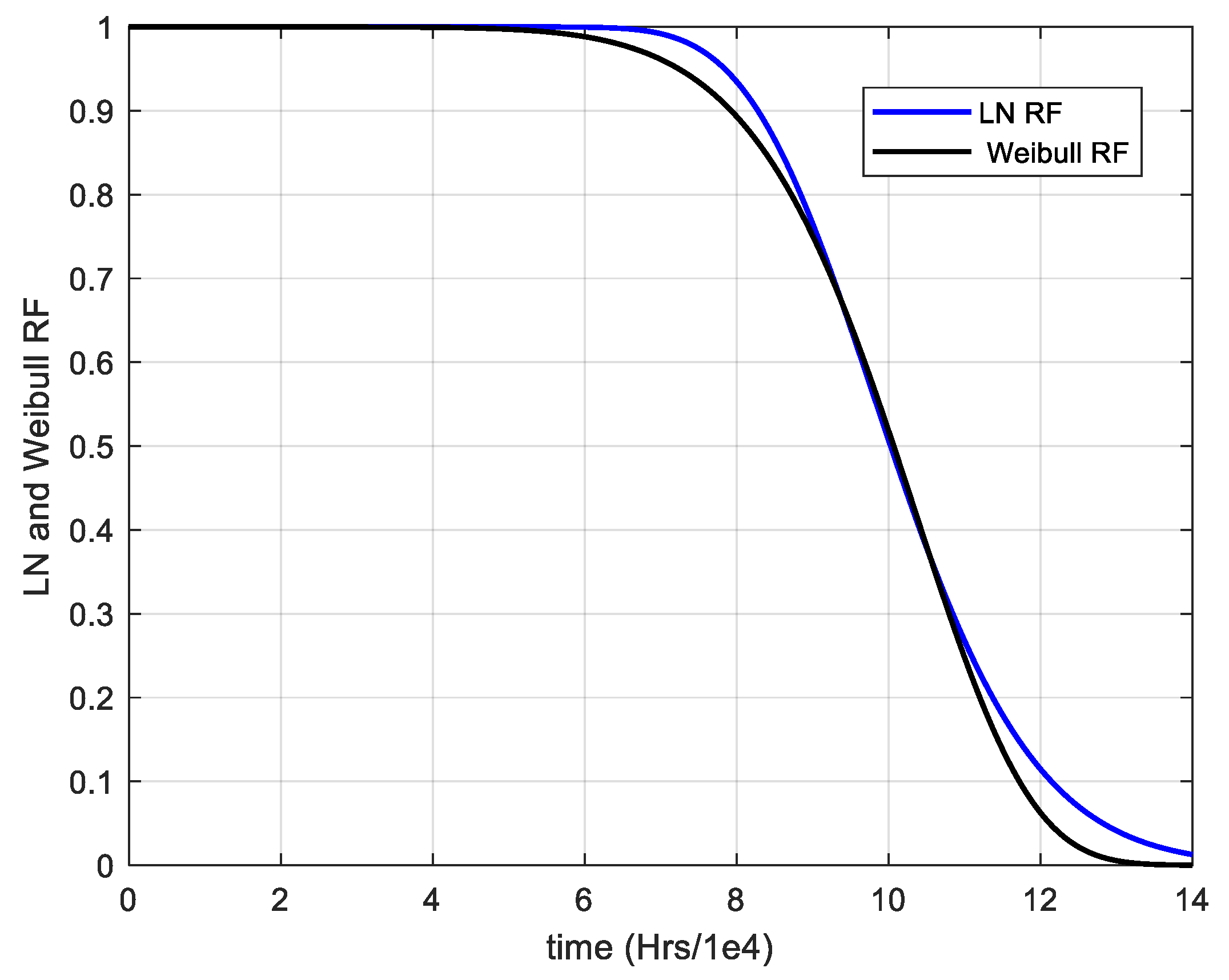
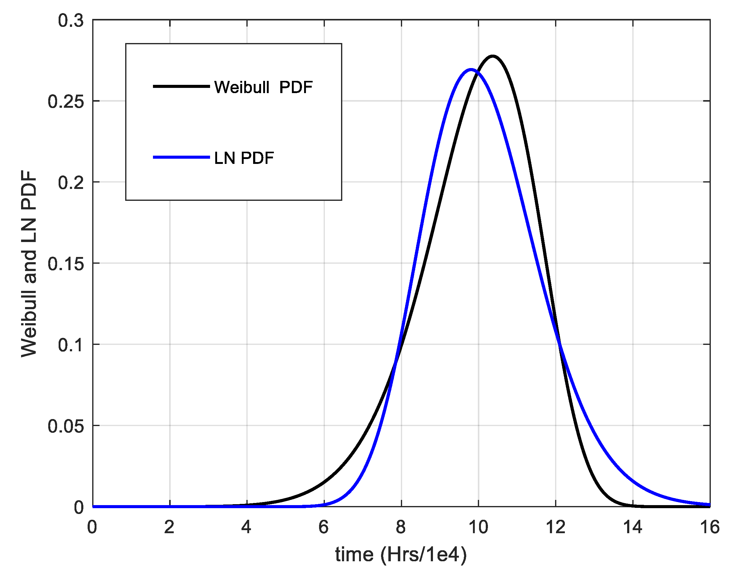
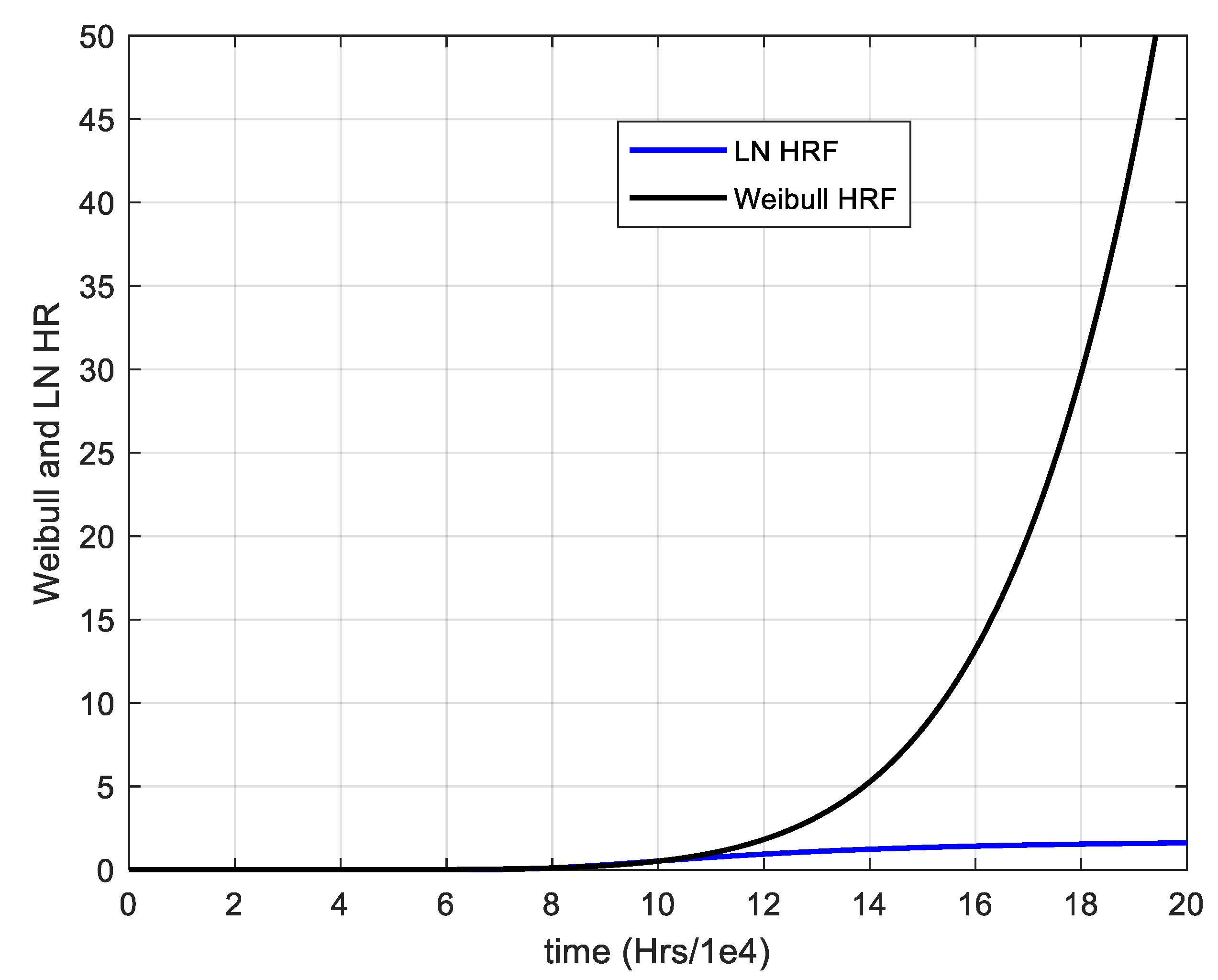
10. On the Consequences of Mistaken Model Identification in Terms of the Hazard Rate Function. A Numerical Example from a Real Dataset

As hinted at above, in this final section (devoted to real data analysis, the data—and the relevant statistical lifetime distribution parameters—being reported in [70]), the consequences, in terms of the hazard rate function behaviour of mistaken model identification are discussed. This is performed by means of a simple numerical and graphical example relevant to real electronics devices’ lifetime data. In this case, the Weibull model is compared first to a LN model, as reported in [70], regarding a comparison of statistical models for the lumen lifetime distribution of high power white Light emitting diode (LED). As highlighted in [70], LED is one of the highly reliable products developed in the past few decades, and significant advances have been reached for the manufacturing technologies of LED. In [70], indeed, it is discusses how traditional reliability assessment techniques have severe limitation on this highly-reliable electronic devices with data few lifetime data; on the other hand, analytical degradation processes models are known for them, which are of great help in evaluating device reliability.
In this application, the authors report that both the LN and Weibull model appear adequate for the statistical fitting of a set of lumen lifetime data (they also consider the Normal model, which will be hinted at afterwards in the following). In particular, the lifetime data are “pseudo failure times”, obtained from the estimated process of a wear model discussed above for lumen data, in eqn. (20). The wear model is extrapolated, for each unit under observation, to the critical failure threshold, which is defined in such application as the one corresponding to a 30% light decrease.
The RF expression of the LN and Weibull models are again reported here. Recalling that Φ(z) denotes the standard Normal CDF for any real number z, the LN RF is expressed as follows (see also (71)):
R(t; ξ,δ)= 1 − Φ[(log(t) − ξ)/δ]
Measuring the lumen lifetime in hours/104, the parameters of the above expression are so estimated from the real data, as reported in [70]: ξ = 2.3054; δ = 0.149415.
The RF expression of the Weibull model here adopted is the W’(θ,β) one of (54):
R(t) = exp[−(t/θ)β]
The following values of the parameters (θ,β) of the above expression also provide a RF which fits very well the same data (again expressed in hours/104): θ = 10.5464, β = 7.890.
The fact that both models are adequate to represent the dataset is confirmed, as reported in [70], by adequate statistical tests, such as the “Akaike Information Criterion” [24], but is also evident graphically. In Figure 1, the RF of the two models (blue curve for the LN, black curve for Weibull model) are reported. In practice, they are almost indistinguishable.
Moreover, the curves of the two corresponding PDFs are reported in Figure 2, which also highlights the very strong similarity of the two models (the time axis has been showed on a larger time interval with respect to Figure 1 for the presence of “large tails” in the two PDF curves).
Such similarity is largely confirmed by the values the p-quantiles (It is recalled that the p-quantile of a given a RV is a value x* such that p100% of the observed value of the RV fall below x*. In the case of a continuous RV as in the present case, if F(x) is the CDF of the RV under study, x* it is the unique solution of F(x*) = p) of the two different reliability models, some of them (for p = 0.05, 0.50, 0.95) are shown in Table 1. As well known, the 0.50-quantile is also known as the Median of the distribution. The two medians, as expected, are equal in practice. It is significant that also the p-quantiles for large values of p (such as p = 0.95) are very close.
On the other hand, the time variations of the two HRF functions are shown in Figure 3, illustrating the remarkable differences between the two models under this respect. Such difference becomes larger and larger as mission times become larger than the median value (t ≈ 10 × 104 h). In order to better appreciate the LN HRF behavior, since its values are much smaller than those of the Weibull one, the curve of the LN HRF alone is also reported in Figure 4. As apparent, for large times the LN HRF tends to become nearly constant (and very slowly decreasing for very large times), while the Weibull one sharply increases.
It is perhaps interesting to remark that in some cases [73] the difference between the HRF for large mission times may be put in relation to the presence of larger tails, and thus larger extreme quantiles (i.e., the p-quantiles with p approaching 1), for the model with a decreasing or a much smaller HRF (as in this case happens to the LN model with respect to the Weibull one). This does not occur in the present application, as already shown, for instance, by the similar values the 0.95 quantiles of the two different reliability models (as it could be anticipated, the 0.95-quantile of the LN model is larger than the 0.95-quantile of the Weibull one, but only marginally, 12.8215 for the LN model vs. 12.1199 for Weibull one).
In conclusion, it can be assessed that—in this and similar cases—if a Weibull model is (wrongly) assumed or estimated instead of a ”true” LN model, the HRF for large mission time maybe grossly overestimated, and such mistake may cause avoidable and costly maintenance actions: indeed, as intuitive in view of the physical meaning of the HRF, maintenance strategies based upon the device’s age are effective only in case of devices possessing an increasing HRF [85,86,87,88,89,90,91,92,93].

11. Conclusions

Aim of the paper is to present a review in reliability studies and applications, which may help in understanding why, even if often contrary to intuition and seldom used in the field of electronics, a decreasing hazard rate function (at least for relatively large mission times) may be the best suited to describe the true model behind a given failure mechanism. This is accomplished by analyzing a review of reasonable physical motivations behind the identification of a reliability model. These motivations lead to the identification of probabilistic life models, originated by the knowledge or estimation of failure mechanisms, and in particular to the so-called “stress-strength” models in order to characterize device “aging”.
This approach may help not only in selecting the “right” reliability model, but has other “practical” application, since the HRF is essential for setting the most adequate maintenance actions on the device.
The author believe that such kind of studies should be further developed, for instance extending the hypotheses assumed for the wear processes (e.g., allowing for non-homogeneous Poisson processes in derivations such as those provided in Section 4), in order to derive possibly even more adequate models for high reliability devices, which offer very few data for a model selection.
It seems also necessary, developing works as in [133], explore more theoretical properties which could establish a closer relation between the device HRF variation in time and the properties of wear acting on the device, as well as developing more complex classes of degradation processes such as the Wiener Process with Random Effects, the Gamma, and the Inverse Gaussian processes [74,133,134,135]. Finally, for lack of space, some other interesting approaches were not illustrated here, but at least two alternative methodologies should be mentioned such as the so-called Multi-State System reliability analysis [136,137,138], and Machine Learning Approach [139,140,141,142].
In the paper we have focused our analysis on Decreasing Hazard Rate models, since there are many cases—which have also been justified on a theoretical basis and illustrated via applicative examples in the former Section—in which a decreasing hazard rate function may be the best suited to describe the true model behind a given failure mechanism (at least for relatively large mission times). Of course, the problem of system degradation is investigated in the literature—also in the field of electronic components—by resorting to approaches different from the one followed here, depending on the various applications. Among these different approaches, one of the possible models for investigating the system degradation is the Multi-State System analysis approach [136,137,138]. In strong summary, Multi-State System reliability analysis is a kind of reliability analysis which considers multiple possible states of the system, whereby both the system and its components are allowed to assume more than two levels of performance. Through multi-state reliability models provide, generally speaking, more realistic and more precise representations of engineering systems, they are much more complex and present major difficulties in system definition and performance evaluation. A suggestion for a further future broadening of the present investigation is thus considering and comparing Multi-State System based approach in reliability analysis with the Decreasing Hazard Rate models.
The Machine Learning approach is based upon a quite different philosophy, which is only minimally related to the probabilistic approach adopted here, since it does not specify a RM; nonetheless, it leads to an “Indirect Reliability Prediction” [142] which is somewhat similar to the “Indirect Reliability Assessment” discussed in the present paper. The Machine Learning Algorithms appear to be adequate, for instance, to power device reliability prediction in extreme conditions, as discussed in [142], and surely appear worth of being further developed for such kind of applications.

Author Contributions

Conceptualization, E.C.; methodology E.C. and G.M.; validation, E.C. and G.M.; formal analysis, E.C. and G.M.; investigation, E.C. and G.M.; writing—original draft preparation, E.C.; writing—review and editing, E.C. and G.M. All authors have read and agreed to the published version of the manuscript.

Funding

This research received no external funding.

Conflicts of Interest

The authors declare no conflict of interest.

Glossary

BSBirnbaum–Saunders (distribution)
CDFCumulative distribution function
CLTCentral limit theorem
CVCoefficient of variation
DHRDecreasing hazard rate
D[Y]Standard deviation of the RV Y
E[Y]Expectation of the RV Y
F( )Generic CDF
f( )Generic PDF
f(x), F(x)PDF and CDF of Stress
g(y), G(y)PDF and CDF of Strength
HRFHazard Rate Function
IDHRFirst increasing, then decreasing hazard rate
IGInverse Gaussian (distribution)
IHRIncreasing hazard rate
IWInverse Weibull (distribution)
LLLog-logistic (distribution)
LNLognormal (distribution)
MTTFMean Time to Failure
N(α,β)Normal (Gaussian) random variable with mean α and standard deviation β
PDFProbability density function
RFReliability function
RMReliability model
R(t)Reliability function at mission time t
RRFResidual reliability function
R(t|s)Residual reliability function at mission time t, for a device aged s time units
RVRandom variable
SD, σStandard deviation
SSStress-Strength
Var, σ2Variance
W(t)Wear process at time t acting on a device
W(α,β)Weibull model with CDF: F(x) = 1 − exp(−αxβ)
W’(θ,β)Weibull alternative form, with CDF: F(x) = 1 − exp(−(x/θ)β)
Γ( )Euler’s Gamma function
μMean value (Expectation)
Φ(z)Standard normal CDF
φ(z)Standard normal PDF
Remark: the symbol “log” always denotes natural logarithm.

References

  1. Chiodo, E.; De Falco, P.; Di Noia, L.P. Challenges and new trends in power electronic devices reliability. Electronics 2021, 10, 925. [Google Scholar] [CrossRef]
  2. Yang, S.; Xiang, D.; Bryant, A.; Mawby, P.; Ran, L.; Tavner, P. Condition monitoring for device reliability in power electronic converters: A review. IEEE Trans. Power Electron. 2010, 25, 2734–2752. [Google Scholar] [CrossRef]
  3. Song, Y.; Wang, B. Survey on reliability of power electronic systems. IEEE Trans. Power Electron. 2012, 28, 591–604. [Google Scholar] [CrossRef]
  4. Wang, H.; Liserre, M.; Blaabjerg, F. Toward reliable power electronics: Challenges, design tools, and opportunities. IEEE Ind. Electron. Mag. 2013, 7, 17–26. [Google Scholar] [CrossRef] [Green Version]
  5. Falck, J.; Felgemacher, C.; Rojko, A.; Liserre, M.; Zacharias, P. Reliability of power electronic systems: An industry perspective. IEEE Ind. Electron. Mag. 2018, 12, 24–35. [Google Scholar] [CrossRef] [Green Version]
  6. Spertino, F.; Amato, A.; Casali, G.; Ciocia, A.; Malgaroli, G. Reliability Analysis and Repair Activity for the Components of 350 kW Inverters in a Large Scale Grid-Connected Photovoltaic System. Electronics 2021, 10, 564. [Google Scholar] [CrossRef]
  7. Sandelic, M.; Sangwongwanich, A.; Blaabjerg, F. Reliability evaluation of PV systems with integrated battery energy storage systems: DC-coupled and AC-coupled configurations. Electronics 2019, 8, 1059. [Google Scholar] [CrossRef] [Green Version]
  8. Liang, Y.; Chen, R.; Han, J.; Wang, X.; Chen, Q.; Yang, H. The study of the single event effect in AlGaN/GaN HEMT based on a cascade structure. Electronics 2021, 10, 440. [Google Scholar] [CrossRef]
  9. Barbagallo, C.; Rizzo, S.A.; Scelba, G.; Scarcella, G.; Cacciato, M. On the lifetime estimation of SiC Power MOSFETs for motor drive applications. Electronics 2021, 10, 324. [Google Scholar] [CrossRef]
  10. Wang, C.; He, Y.; Wang, C.; Li, L.; Wu, X. Multi-chip IGBT module failure monitoring based on module transconductance with temperature calibration. Electronics 2020, 9, 1559. [Google Scholar] [CrossRef]
  11. Wang, C.; He, Y.; Wang, C.; Wu, X.; Li, L. A fusion algorithm for online reliability evaluation of microgrid inverter IGBT. Electronics 2020, 9, 1294. [Google Scholar] [CrossRef]
  12. Wei, J.; Li, Z.; Li, B. Investigation of reverse recovery current of high-power thyristor in pulsed power supply. Electronics 2020, 9, 1292. [Google Scholar] [CrossRef]
  13. Mazzanti, G.; Diban, B.; Chiodo, E.; De Falco, P.; Di Noia, L.P. Forecasting the reliability of components subjected to harmonics generated by power electronic converters. Electronics 2020, 9, 1266. [Google Scholar] [CrossRef]
  14. Lee, C.-T.; Ho, P.-T. Energy-saving research on new type of LED sensor lamp with low-light mode. Electronics 2020, 9, 1649. [Google Scholar] [CrossRef]
  15. Pinti, F.; Belli, A.; Palma, L.; Gattari, M.; Pierleoni, P. Validation of forward voltage method to estimate cracks of the solder joints in high power LED. Electronics 2020, 9, 920. [Google Scholar] [CrossRef]
  16. Susinni, G.; Rizzo, S.A.; Iannuzzo, F. Two decades of condition monitoring methods for power devices. Electronics 2021, 10, 683. [Google Scholar] [CrossRef]
  17. Barlow, R.E.; Proschan, F. Statistical Theory of Reliability and Life Testing; Holt, Rinehart & Winston: New York, NY, USA, 1975. [Google Scholar]
  18. Billinton, R.; Allan, R.N. Reliability Evaluation of Engineering Systems: Concepts and Techniques; Plenum Press: New York, NY, USA, 1992. [Google Scholar]
  19. Lewis, E.E. Introduction to Reliability Engineering; Wiley: New York, NY, USA, 1987. [Google Scholar]
  20. Birolini, A. Reliability Engineering: Theory and Practice; Springer: Berlin, Germany, 2014. [Google Scholar]
  21. Catuneanu, V.M.; Mihalache, A.N. Reliability Fundamentals; Elsevier: Amsterdam, The Netherlands, 1989. [Google Scholar]
  22. Cox, D.R.; Oakes, D. Analysis of Survival Data; Chapman & Hall: London, UK, 1984. [Google Scholar]
  23. Cohen, A.C.; Whitten, B.J. Parameter Estimation in Reliability and Life Span Models; Marcel Dekker: New York, NY, USA, 1988. [Google Scholar]
  24. Crowder, M.J.; Kimber, A.C.; Smith, R.L.; Sweeting, T.J. Statistical Methods of Reliability Data; Chapman and Hall: London, UK, 1991. [Google Scholar]
  25. Ushakov, I.A.; Harrison, R.A. Handbook of Reliability Engineering; Wiley: New York, NY, USA, 1994. [Google Scholar]
  26. Hoyland, A.; Rausand, M. System Reliability Theory; Wiley: New York, NY, USA, 2003. [Google Scholar]
  27. Kalbfleisch, J.D.; Prentice, R.L. The Statistical Analysis of Failure Time Data; Wiley: New York, NY, USA, 2002. [Google Scholar]
  28. Lawless, J.F. Statistical Models and Methods for Lifetime Data; Wiley: New York, NY, USA, 1982. [Google Scholar]
  29. Lazzaroni, M. Reliability Engineering; Springer: Berlin/Heidelberg, Germany, 2011. [Google Scholar]
  30. Mann, N.; Schafer, R.E.; Singpurwalla, N.D. Methods for Statistical Analysis of Reliability and Life Data; Wiley: New York, NY, USA, 1974. [Google Scholar]
  31. Martz, H.F.; Waller, R.A. Bayesian Reliability Analysis; Krieger Publishing: Malabar, FL, USA, 1991. [Google Scholar]
  32. Modarres, M. Reliability and Risk Analysis; M. Dekker: New York, NY, USA, 1993. [Google Scholar]
  33. Meeker, W.Q.; Escobar, L.A. Statistical Methods for Reliability Data; Wiley: New York, NY, USA, 1998. [Google Scholar]
  34. Nelson, W. Applied Life Data Analysis; Wiley: New York, NY, USA, 1982. [Google Scholar]
  35. Nelson, W. Accelerated Testing; Wiley: New York, NY, USA, 1990. [Google Scholar]
  36. Singpurwalla, N.D. Reliability and Risk: A Bayesian Perspective; Wiley Series in Probability and Statisticsl; Wiley: New York, NY, USA, 2006. [Google Scholar]
  37. Krishnaiah, P.R.; Rao, C.R. (Eds.) Handbook of Statistics, Vol. 7: Quality Control and Reliability; North Holland: Amsterdam, The Netherlands, 1988. [Google Scholar]
  38. Hamada, M.S.; Wilson, A.; Reese, C.S.; Martz, H. Bayesian Reliability; Springer: Berlin/Heidelberg, Germany, 2008. [Google Scholar]
  39. Prabhakar Murthy, D.N.; Rausand, M.; Østerås, T. Product Reliability: Specification and Performance; Springer: London, UK, 2008. [Google Scholar]
  40. Wang, C. Structural Reliability and Time-Dependent Reliability; Springer: Berlin/Heidelberg, Germany, 2021. [Google Scholar]
  41. Verma, A.K.; Ajit, S.; Karanki, D.R. Reliability and Safety Engineering; Springer: Berlin/Heidelberg, Germany, 2010. [Google Scholar]
  42. Grynchenko, O.; Alfyorov, O. Mechanical Reliability; Springer: Berlin/Heidelberg, Germany, 2020. [Google Scholar]
  43. Barlow, R.E.; Claroti, C.A.; Spizzichino, F. Reliability and Decision Making; Chapman & Hall: London, UK, 1993. [Google Scholar]
  44. Ibrahim, J.G.; Chen, M.H.; Sinha, D. Bayesian Survival Analysis; Springer: Berlin/Heidelberg, Germany, 2011. [Google Scholar]
  45. Johnson, N.L.; Kotz, S.; Balakrishnan, N. Continuous Univariate Distributions, 2nd ed.; Wiley: New York, NY, USA, 1995; Volumes 1 and 2. [Google Scholar]
  46. Esary, J.D.; Marshall, A.W. Shock models and wear processes. Ann. Probab. 1973, 1, 627–649. [Google Scholar] [CrossRef]
  47. Lu, C.J.; Meeker, W.Q. Using degradation measures to estimate a time-to-failure distribution. Technometrics 1993, 35, 161–174. [Google Scholar] [CrossRef]
  48. Lu, C.J.; Meeker, W.Q.; Escobar, L.A. A comparison of degradation and failure-time analysis methods for estimating a time-to-failure distribution. Stat. Sin. 1996, 6, 531–554. [Google Scholar]
  49. Abdel-Hameed, A. A Gamma wear process. IEEE Trans. Reliab. 1975, 24, 152–153. [Google Scholar] [CrossRef]
  50. Dasgupta, A.; Pecht, M. Material failure mechanisms and damage models. IEEE Trans. Reliab. 1991, 40, 531–536. [Google Scholar] [CrossRef]
  51. Cinlar, E. Seminar on Stochastic Processes; 3Island Press, 1990; Available online: https://www.springer.com/gp/book/9780817634889 (accessed on 8 September 2021).
  52. Durham, S.D.; Padgett, W.J. Cumulative damage models for system failure with application to carbon fibers and composites. Technometrics 1997, 39, 34–44. [Google Scholar] [CrossRef]
  53. Si, X.; Zhou, D. A generalized result for degradation model-based reliability estimation. IEEE Trans. Autom. Sci. Engin. 2014, 11, 632–637. [Google Scholar] [CrossRef]
  54. Singpurwalla, N.D. Gamma processes and their generalizations: An overview. In Engineering Probabilistic Design and Maintenance for Flood Protection; Cooke, R., Mendel, M., Vrijling, H., Eds.; Kluwer Academic Publishers: Dordrecht, The Netherlands, 1997; pp. 67–75. [Google Scholar]
  55. Van Noortwijk, J.M.; Pandey, M.D. A stochastic deterioration process for time-dependent reliability analysis. In Reliability and Optimization of Structural Systems; Maes, M.A., Huyse, L., Eds.; Taylor & Francis: London, UK, 2004; pp. 259–265. [Google Scholar]
  56. Van Noortwijk, J.M.; van der Weide, J.A.; Kallen, M.J.; Pandey, M.D. Gamma processes and peaks-over-threshold distributions for time-dependent reliability. Reliab. Eng. Syst. Saf. 2007, 92, 1651–1658. [Google Scholar] [CrossRef]
  57. Van Noortwijk, J.M. A survey of the application of Gamma processes in maintenance. Reliab. Eng. Syst. Saf. 2009, 94, 2–21. [Google Scholar] [CrossRef]
  58. Dasgupta, A.; Pecht, M. Physics of failure: An approach to reliable product development. J. Inst. Environ. Sci. 1995, 38, 30–34. [Google Scholar]
  59. Vichare, N.M.; Pecht, M. Prognostics and health management of electronics. IEEE Trans. Comp. Packag. Technolog. 2006, 29, 222–229. [Google Scholar] [CrossRef]
  60. Roman, D.; Saxena, S.; Bruns, J.; Valentin, R.; Pecht, M.; Flynn, D. A machine learning degradation model for electrochemical capacitors operated at high temperature. IEEE Access 2021, 9, 25544–25553. [Google Scholar] [CrossRef]
  61. Menon, S.; Chen, D.Y.; Osterman, M.; Pecht, M. Copper trace fatigue life modeling for rigid electronic assemblies. IEEE Trans. Device Mater. Reliab. 2021, 21, 79–86. [Google Scholar] [CrossRef]
  62. Lee, C.; Jo, S.; Kwon, D.; Pecht, M. Capacity-fading behavior analysis for early detection of unhealthy Li-ion batteries. IEEE Trans. Ind. Electron. 2021, 68, 2659–2666. [Google Scholar] [CrossRef]
  63. Qi, H.; Osterman, M.; Pecht, M. A rapid life-prediction approach for PBGA solder joints under combined thermal cycling and vibration loading conditions. IEEE Trans. Comp. Packag. Technolog. 2009, 32, 283–292. [Google Scholar] [CrossRef]
  64. Pecht, M. Prognostics and health monitoring for improved qualification. In Proceedings of the 10th International Conference on Thermal, Mechanical and Multi-Physics Simulation and Experiments in Microelectronics and Microsystems (EuroSimE 2009), Delft, The Netherlands, 26–29 April 2009; pp. 1–10. [Google Scholar]
  65. Jaai, R.; Pecht, M.; Cook, J. Detecting failure precursors in BGA solder joints. In Proceedings of the 2009 Annual Reliability and Maintainability Symposium, Fort Worth, TX, USA, 26–29 January 2009; pp. 100–105. [Google Scholar] [CrossRef] [Green Version]
  66. Cheng, S.; Pecht, M. A fusion prognostics method for remaining useful life prediction of electronic products. In Proceedings of the 2009 IEEE International Conference on Automation Science and Engineering, Bangalore, India, 22–25 August 2009; pp. 102–107. [Google Scholar]
  67. Pecht, M.; Tuchband, B.; Vichare, N.; Ying, Q.J. Prognostics and health monitoring of electronics. In Proceedings of the 2007 International Conference on Thermal, Mechanical and Multi-Physics Simulation Experiments in Microelectronics and Micro-Systems (EuroSime 2007), London, UK, 16–18 April 2007; pp. 1–8. [Google Scholar]
  68. Gu, J.; Pecht, M. Prognostics and health management using physics-of-failure. In Proceedings of the 2008 Annual Reliability and Maintainability Symposium, Las Vegas, NV, USA, 28–31 January 2008; pp. 481–487. [Google Scholar]
  69. Gu, J.; Pecht, M. Predicting the reliability of electronic products. In Proceedings of the 2007 8th International Conference on Electronic Packaging Technology, Shanghai, China, 14–17 August 2007; pp. 1–8. [Google Scholar]
  70. Fan, J.; Yung, K.C.; Pecht, M. Comparison of statistical models for the lumen lifetime distribution of high power white LEDs. In Proceedings of the IEEE 2012 Prognostics and System Health Management Conference, Beijing, China, 23–25 May 2012; pp. 1–7. [Google Scholar]
  71. Si, X.; Chang-Hua, H.; Wang, W.; Zhou, D. A Wiener-process-based degradation model with a recursive filter algorithm for remaining useful life estimation. Mech. Syst. Sign. Process. 2013, 35, 219–237. [Google Scholar] [CrossRef]
  72. Ebrahimi, N.B. Indirect assessment of system reliability. IEEE Trans. Reliab. 2003, 52, 58–62. [Google Scholar] [CrossRef]
  73. Chiodo, E.; Mazzanti, G. Mathematical and physical properties of reliability models in view of their application to modern power system components. In Innovations in Power Systems Reliability; Anders, G.J., Vaccaro, A., Eds.; Springer: Berlin/Heidelberg, Germany, 2011; pp. 59–140. [Google Scholar]
  74. Chen, D.; Lio, Y.; Ng, H.K.T.; Tsai, T. Statistical Modeling for Degradation Data; Springer: Berlin/Heidelberg, Germany, 2017. [Google Scholar]
  75. Erto, P. (Ed.) Statistics for Innovation; Springer: Milan, Italy, 2009. [Google Scholar]
  76. Xie, L.; Wang, L. Reliability Degradation of Mechanical Components and Systems. In Handbook of Performability Engineering; Misra, B.K., Ed.; Springer: Berlin/Heidelberg, Germany, 2008. [Google Scholar]
  77. Cha, J.H.; Finkelstein, M. On new classes of extreme shock models and some generalizations. J. Appl. Probab. 2011, 48, 258–270. [Google Scholar] [CrossRef]
  78. Finkelstein, M.; Gertsbakh, I. On preventive maintenance of systems subject to shocks. J. Risk Reliab. 2015, 230, 220–227. [Google Scholar] [CrossRef]
  79. Gertsbakh, I.; Shpungin, Y. Network Reliability and Resilience; Springer: Berlin, Germany, 2011. [Google Scholar]
  80. Lai, C.D.; Xie, M. Stochastic Aging and Dependence for Reliability; Springer: New York, NY, USA, 2006. [Google Scholar]
  81. Cinlar, E. Introduction to Stochastic Processes; Prentice-Hall: Englewood Cliffs, NJ, USA, 1975. [Google Scholar]
  82. Thompson, W.A. Point Process Models with Applications to Safety and Reliability; Chapman and Hall: London, UK, 1988. [Google Scholar]
  83. Aven, T.; Jensen, U. Stochastic Models in Reliability; Springer: Berlin, Germany, 1999. [Google Scholar]
  84. Cha, J.H.; Finkelstein, M. Point Processes for Reliability Analysis Shocks and Repairable Systems; Springer: Berlin/Heidelberg, Germany, 2018. [Google Scholar]
  85. Gertsbakh, I. Reliability Theory with Applications to Preventive Maintenance; Springer: Berlin/Heidelberg, Germany, 2020. [Google Scholar]
  86. Mobley, K. An Introduction to Predictive Maintenance; Butterworth-Heinemann: Oxford, UK, 2002. [Google Scholar]
  87. Narayana, V. Effective Maintenance Management: Risk and Reliability Strategies for Optimizing Performance; Industrial Press, Inc.: New York, NY, USA, 2004. [Google Scholar]
  88. Nakagawa, T. Maintenance Theory of Reliability; Springer: London, UK, 2005. [Google Scholar]
  89. Bloom, N.B. Reliability Centered Maintenance: Implementation Made Simple; McGraw-Hill: New York, NY, USA, 2005. [Google Scholar]
  90. Hongzhou, W.; Hoang, P. Reliability and Optimal Maintenance; Springer: Berlin/Heidelberg, Germany, 2006. [Google Scholar]
  91. Murthy, D.N.P.; Blischke, W.R. Warranty Management and Product Manufacture; Springer: London, UK, 2006. [Google Scholar]
  92. Jardine, A.K.S.; Tsang, A.H.C. Maintenance, Replacement, and Reliability: Theory and Applications; Taylor & Francis: Boca Raton, FL, USA, 2006. [Google Scholar]
  93. Misra, K.B. Maintenance Engineering and Maintainability. An Introduction. In Handbook of Performability Engineering; Springer: Berlin/Heidelberg, Germany, 2008; Chapter 46. [Google Scholar]
  94. Denson, W. Handbook of 217plus Reliability Prediction Models; The Reliability Information Analysis Center: Utica, NY, USA, 2006; 217p. [Google Scholar]
  95. Harms, J.W. Revision of MIL-HDBK-217, Reliability prediction of electronic equipment. In Proceedings of 2010 Annual Reliability and Maintainability Symposium (RAMS), Tucson, AZ, USA, 24–27 January 2010; pp. 1–3. [Google Scholar]
  96. Wong, K.L. What is wrong with the existing reliability prediction methods? Qual. Reliab. Eng. Int. 1990, 6, 251–258. [Google Scholar] [CrossRef]
  97. Pecht, M.; Kang, W.C. A critique of MIL-Hdbk-217E reliability prediction methods. IEEE Trans. Reliab. 1988, 37, 453–457. [Google Scholar] [CrossRef]
  98. Glaser, R.E. Bathtub and related failure rate characterizations. J. Amer. Statist. Assoc. 1980, 75, 667–672. [Google Scholar] [CrossRef]
  99. Gaonkar, A.; Patil, R.B.; Kyeong, S.; Das, D.; Pecht, M. An assessment of validity of the bathtub model hazard rate trends in electronics. IEEE Access 2021, 9, 10282–10290. [Google Scholar] [CrossRef]
  100. Kotz, S.; Lumelskii, Y.; Pensky, M. The Stress-Strength Model and its Generalizations: Theory and Applications; Imperial College Press: London, UK, 2003. [Google Scholar]
  101. Johnson, R.A. Stress-Strength models for reliability. In Handbook of Statistics, Vol. 7: Quality Control and Reliability; Krishnaiah, P.R., Rao, C.R., Eds.; North Holland: Amsterdam, The Netherlands, 1988. [Google Scholar]
  102. Huang, W.; Askin, R.G. A generalized SSI reliability model considering stochastic loading and strength aging degradation. IEEE Trans. Reliab. 2004, 53, 77–82. [Google Scholar] [CrossRef]
  103. Lewis, E.E.; Chen, H.C. Load-capacity interference and the bathtub curve. IEEE Trans. Reliab. 1994, 43, 470–475. [Google Scholar] [CrossRef]
  104. Chiodo, E.; Mazzanti, G. Bayesian reliability estimation based on a Weibull stress-strength model for aged power system components subjected to voltage surges. IEEE Trans. Dielectr. Electr. Insul. 2006, 13, 146–159. [Google Scholar] [CrossRef]
  105. Chang, D.S.; Tang, L.C. Reliability bounds and critical time for the Birnbaum-Saunders distribution. IEEE Trans. Reliab. 1993, 42, 464–469. [Google Scholar] [CrossRef]
  106. Desmond, A. On the relationship between two fatigue-life models. IEEE Trans. Reliab. 1986, 35, 167–169. [Google Scholar] [CrossRef]
  107. Kundu, D.; Kannan, N.; Balakrishnan, N. On the hazard function of Birnbaum-Saunders distribution and associated inference. Comput. Stat. Data Anal. 2008, 52, 26–52. [Google Scholar] [CrossRef] [Green Version]
  108. Chhikara, R.S.; Folks, J.L. The Inverse Gaussian Distribution; Marcel Dekker: New York, NY, USA, 1989. [Google Scholar]
  109. Iyengar, S.; Patwardhan, G. Recent developments in the Inverse Gaussian distribution. In Handbook of Statistics, Vol. 7: Quality Control and Reliability; Krishnaiah, P.R., Rao, C.R., Eds.; North Holland: Amsterdam, The Netherlands, 1988; pp. 479–490. [Google Scholar]
  110. Chiodo, E.; Del Pizzo, A.; Di Noia, L.P.; Lauria, D. Modeling and Bayes estimation of battery lifetime for smart grids under an Inverse Gaussian model. Int. Rev. Electr. Eng. 2013, 8, 1253–1266. [Google Scholar]
  111. Whitmore, G. Estimating degradation by a Wiener diffusion process subject to measurement error. Lifetime Data Anal. 1995, 1, 307–319. [Google Scholar] [CrossRef] [PubMed]
  112. Erto, P. Genesis, properties and identification of the Inverse Weibull survival model. Stat. Appl. 1989, 1, 117–128. (In Italian) [Google Scholar]
  113. Erto, P.; Palumbo, B. Origins, properties and parameters estimation of the hyperbolic reliability model. IEEE Trans. Reliab. 2005, 54, 276–281. [Google Scholar] [CrossRef]
  114. Tadikamalla, P.R.; Johnson, N.L. Systems of frequency curves generated by transformations of logistic variables. Biometrika 1982, 69, 461–465. [Google Scholar] [CrossRef]
  115. Tadikamalla, P.R. A Look at the Burr and related distributions. Int. Stat. Rev. 1980, 48, 337–344. [Google Scholar] [CrossRef]
  116. Bennett, S. Log-Logistic regression models for survival data. J. Royal Stat. Soc. Ser. C 1983, 32, 165–171. [Google Scholar] [CrossRef]
  117. Srivastava, P.W.; Shukla, R. A Log-Logistic step-stress model. IEEE Trans. Reliab. 2008, 57, 431–434. [Google Scholar] [CrossRef]
  118. Crow, E.L.; Shimizu, K. Lognormal Distributions; Marcel Dekker: New York, NY, USA, 1988. [Google Scholar]
  119. Sweet, A.L. On the hazard rate of the lognormal distribution. IEEE Trans. Reliab. 1990, 39, 325–328. [Google Scholar] [CrossRef]
  120. Dumonceaux, R.; Antle, C.E. Discrimination between the Lognormal and Weibull distributions. Technometrics 1973, 15, 923–926. [Google Scholar] [CrossRef]
  121. Lawless, J.F. Statistical models in reliability. Technometrics 1983, 25, 305–335. [Google Scholar] [CrossRef]
  122. Croes, K.; Manca, J.V. The time of guessing your failure time distribution is over. Microelectron. Reliab. 1988, 38, 1187–1191. [Google Scholar] [CrossRef]
  123. Desmond, A. Stochastic models of failure in random environments. Can. J. Stat. 1985, 13, 171–183. [Google Scholar] [CrossRef]
  124. Press, S.J. Subjective and Objective Bayesian Statistics: Principles, Models, and Applications, 2nd ed.; Wiley: New York, NY, USA, 2002. [Google Scholar]
  125. Roy, D.; Mukherjee, S.P. Generalized mixtures of exponential distributions. J. Appl. Prob. 1988, 25, 510–518. [Google Scholar] [CrossRef]
  126. Proschan, F. Theoretical explanation of observed decreasing failure rate. Technometrics 1963, 5, 375–383. [Google Scholar] [CrossRef]
  127. Mi, J. A new explanation of decreasing failure rate of a mixture of exponentials. IEEE Trans. Reliab. 1998, 47, 460–462. [Google Scholar]
  128. Follmann, D.A.; Goldberg, M.S. Distinguishing heterogeneity from decreasing hazard rate. Technometrics 1988, 30, 389–396. [Google Scholar] [CrossRef]
  129. Shimi, I.N. System failures and stochastic hazard rate. In Applications of Statistics; Krishnaiah, P.R., Ed.; North Holland: New York, NY, USA, 1977; pp. 497–505. [Google Scholar]
  130. Harris, C.M.; Singpurwalla, N.D. Life distributions derived from stochastic hazard function. IEEE Trans. Reliab. 1967, 17, 70–79. [Google Scholar] [CrossRef]
  131. Heckman, J.J.; Singer, B. Population heterogeneity in demographic models. In Multidimensional Mathematical Demography; Land, K.C., Rogers, A., Eds.; Academic Press: New York, NY, USA, 1982. [Google Scholar]
  132. Lindley, D.V.; Singpurwalla, N.D. Multivariate distributions for the life lengths of components of a system sharing a common environment. J. Appl. Prob. 1986, 23, 418–431. [Google Scholar] [CrossRef]
  133. Gebraeel, N.; Elwany, A.; Pan, J. Residual life predictions in the absence of prior degradation knowledge. IEEE Trans. Reliab. 2009, 58, 106–117. [Google Scholar] [CrossRef]
  134. Cinlar, E. On a generalization of Gamma processes. J. Appl. Prob. 1980, 17, 467–480. [Google Scholar] [CrossRef]
  135. Zheng, W.; Liyang, X. Dynamic Reliability Model of Components Under Random Load. IEEE Trans. Reliab. 2009, 57, 474–479. [Google Scholar] [CrossRef]
  136. Barlow, R.; Wu, E.; Alexander, S. Coherent system with multi-state components. Math. Oper. Res. 1978, 3, 275–281. [Google Scholar] [CrossRef] [Green Version]
  137. Faghih-Roohi, S.; Xie, M.; Ng, K.M.; Yam, R.C.M. Dynamic availability assessment and optimal component design of multi-state weighted k-out-of-n systems. Reliab. Eng. Syst. Saf. 2014, 123, 57–62. [Google Scholar] [CrossRef]
  138. Zaitseva, E.; Levashenko, V. Reliability analysis of multi-state system with application of multiple-valued logic. Int. J. Qual. Reliab. Manag. 2017, 34, 862–878. [Google Scholar] [CrossRef]
  139. Alsina, E.F.; Chica, M.; Trawiński, K.; Regattieri, A. On the use of machine learning methods to predict component reliability from datadriven industrial case studies. Int. J. Adv. Manuf. Technol. 2018, 94, 2419–2433. [Google Scholar] [CrossRef]
  140. Zheng, Y.; Wu, L.; Li, X.; Yin, C. A relevance vector machine-based approach for remaining useful life prediction of power MOSFETs. In Proceedings of the 2014 Prognostics and System Health Management Conference (PHM-2014 Hunan), Zhangiiaijie City, China, 24–27 August 2014; pp. 642–646. [Google Scholar]
  141. McMenemy, D.; Chen, W.; Zhang, L.; Pattipati, K.; Bazzi, A.M.; Joshi, S. A Machine Learning Approach for Adaptive Classification of Power MOSFET Failures. In Proceedings of the 2019 IEEE Transportation Electrification Conference and Expo (ITEC), Detroit, MI, USA, 19–21 June 2019; pp. 1–8. [Google Scholar]
  142. Olivares, C.A.; Rahman, R.; Stankus, C.; Hampton, J.; Zedwick, A.; Ahmed, M. Predicting Power Electronics Device Reliability under Extreme Conditions with Machine Learning Algorithms. arXiv 2021, arXiv:2107.10292. [Google Scholar]
Figure 1. The RF curves of the LN and Weibull models for lumen data after [70].
Electronics 10 02553 g001
Figure 2. The PDF curves of the LN and Weibull models for lumen data after [70].
Electronics 10 02553 g002
Figure 3. The two HRF corresponding to the two RF of Figure 1 and PDF of Figure 2.
Electronics 10 02553 g003
Figure 4. The HRF curves of the LN model for lumen data.
Electronics 10 02553 g004
Table 1. Values of some p-quantiles of the LN and the Weibull reliability models for lumen data after [70] (for p = 0.05, 0.50, 0.95).
pLNWeibull
0.057.84287.2379
0.5010.027810.0677
0.9512.821512.1199
Publisher’s Note: MDPI stays neutral with regard to jurisdictional claims in published maps and institutional affiliations.

