Analysis and Recognition of Human Lower Limb Motions Based on Electromyography (EMG) Signals

Abstract

Background: This paper focuses on the characteristics of lower limb EMG signals for common movements. Methods: We obtained length data for lower limb muscles during gait motion using software named OpenSim; statistical product and service solutions (SPSS) were utilized to study the correlation between each muscle, based on gait data. Low-correlation muscles in different regions were selected; inertial measurement unit (IMU) and EMG sensors were used to measure the lower limb angles and EMG signals when on seven kinds of slope, in five kinds of gait (walking on flat ground, uphill, downhill, up-step and down-step) and four kinds of movement (squat, lunge, raised leg and standing up). Results: After data denoising and feature extraction, we designed a double hidden-layer BP neural network to recognize the above motions according to EMG signals. Results show that EMG signals of selected muscles have a certain periodicity in the process of movement that can be used to identify lower limb movements. Conclusions: It can be seen, after the recognition of different proportions of training and testing sets that the average recognition rate of the BP neural network is 86.49% for seven gradients, 93.76% for five kinds of gait and 86.07% for four kinds of movements.

1. Introduction

Human motion intention recognition technology offers a way to use physical methods, through all kinds of sensor systems, to identify human motion modes and gait divisions. It has important applications in many fields, which has brought widespread interest around the world [1]. For example, famous scientists have applied human motion intention technology to the development of exoskeletons and soft exo-suits, enabling a cold auxiliary wearable device to recognize the wearer’s motion intention faster and more actively, and cooperate with the wearer in time, so as to help the human wearer to complete tasks in more complex and dangerous environments [2,3]. Therefore, it is essential to research more accurate human motion-sensing technology [3]. Nowadays, the methods used to recognize human motion information mainly include bio-force information (such as joint angle, plantar pressure, joint torque, etc.), video imaging and bioelectrical signals (such as in an electrocardiogram (ECG), electrooculogram (EOG), electromyography (EMG), etc.) [4,5,6,7]. Biological force information can only reflect the characteristics of human static motion while failing to predict human motion. Force sensors and pose sensors have the advantages of small volume and low power consumption. However, they cannot be directly integrated into the wearer’s body like bioelectrical signal sensors; therefore, users cannot wear them without their feeling like a foreign body, and the recognition rate for motion still needs to be further improved [4]. Image recognition technology needs specialized field and camera equipment to complete the collation of human motion information; it is usually applied in the context of personnel monitoring [5]. Some researchers have also attempted to use computer vision technology to detect the wearer’s surroundings and environment as a way to enable wearable devices to recognize road conditions. The authors of [6] designed a sub-vision system in a knee prosthesis, which provided environmental information for the motion-control system of amputees and reconstructed the visual system circuit, by which the recognition and motion prediction of different road conditions are realized [6]. A camera was installed on the experimenter’s glasses and knee joint in another study [7], and Bayesian theory and modern deep neural networks were used to identify different road conditions such as grass and steps [7]. However, computer vision technology has high requirements in terms of camera accuracy and stability, and the cost of products is still high, whether for research or production. Because of its convenient detection, non-invasive nature, and response ahead of movement (an EMG signal is transmitted 30–150 ms earlier than movement), bioelectrical signals have gradually become the mainstream research object in the field of human–computer interaction [8,9]. A surface electromyography (EMG) signal, as the superposition of motor unit action potential in time and space, is a comprehensive effect of EMG and the neural stem on the skin surface, one that can reflect neuromuscular activity to a certain extent [8]. It is one of the bioelectrical signals that can most easily be obtained [9,10]. When the EMG electrode is placed on the skin surface of a human body, it can record the weak potential difference on the skin surface that is caused by muscle contraction; then, the EMG signal for analysis is generated after amplification and running through a conversion circuit. Because the EMG signal is generated before the movement occurs, and it presents different waveforms and periodicity with different motion modes, it offers inherent advantages for motion recognition [11]. However, the research of human motion recognition based on an EMG signal is still in the preliminary stages, because the EMG signal is weak and difficult to analyze [11]. Due to the large number of lower limb muscles, some muscles must cooperate to complete a single movement, and one muscle can also perform different joint movements (such as the gastrocnemius participating in both knee flexion and ankle plantar flexion) [12]. Therefore, the optimal combination of lower limb skeletal muscle, which can best reflect the joint movement, is also one of the methods to improve movement intention recognition.

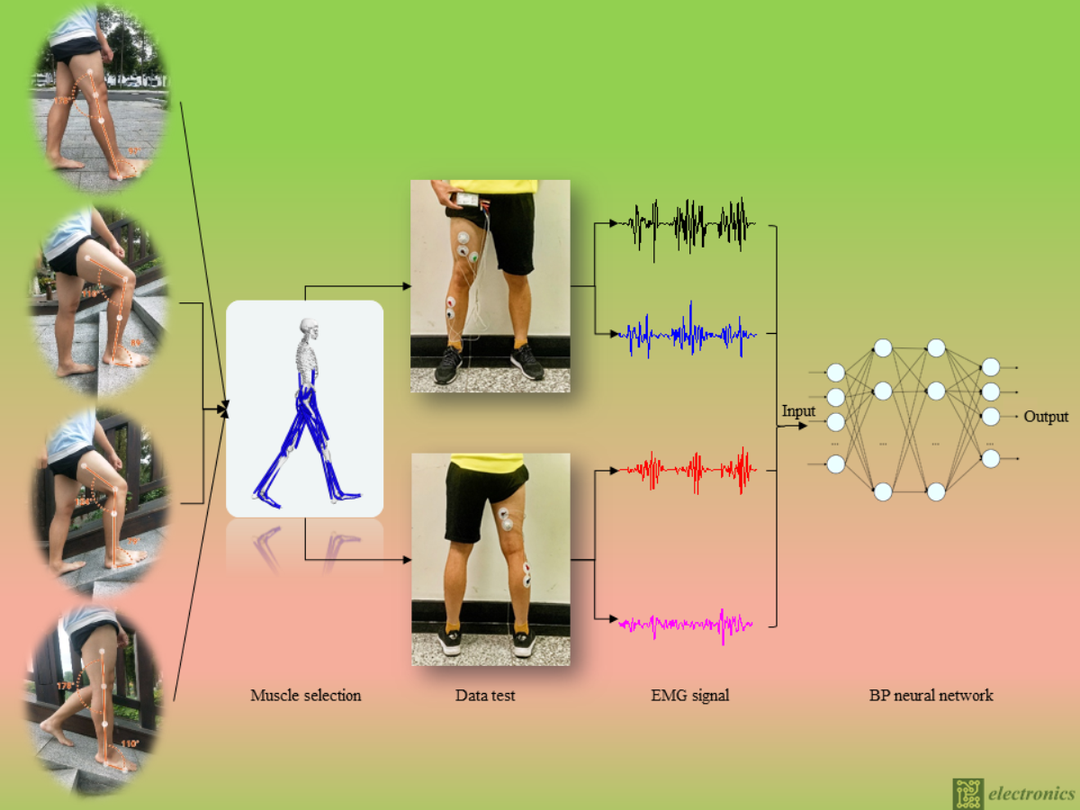
We proceeded as follows to select the appropriate muscles to measure EMG signals and to verify their feasibility for identifying different lower-limb movements. Firstly, the data for the length change of lower limb muscles in the process of gait movement were obtained using the OpenSim musculoskeletal simulation software. Then, SPSS was utilized to analyze the correlations among those data, the selected muscles (including the rectus femoris, biceps femoris, tibialis anterior muscle and gastrocnemius) being related to lower limb movement but irrespective of length change. In Section 2, IMU and EMG sensors were applied to collect the angle data and EMG data during exercise. After de-noising and feature extraction in Section 3, the signals are devoted to identifying seven kinds of slopes, five kinds of gait, and four kinds of movements. This paper’s structure is shown in Figure 1.

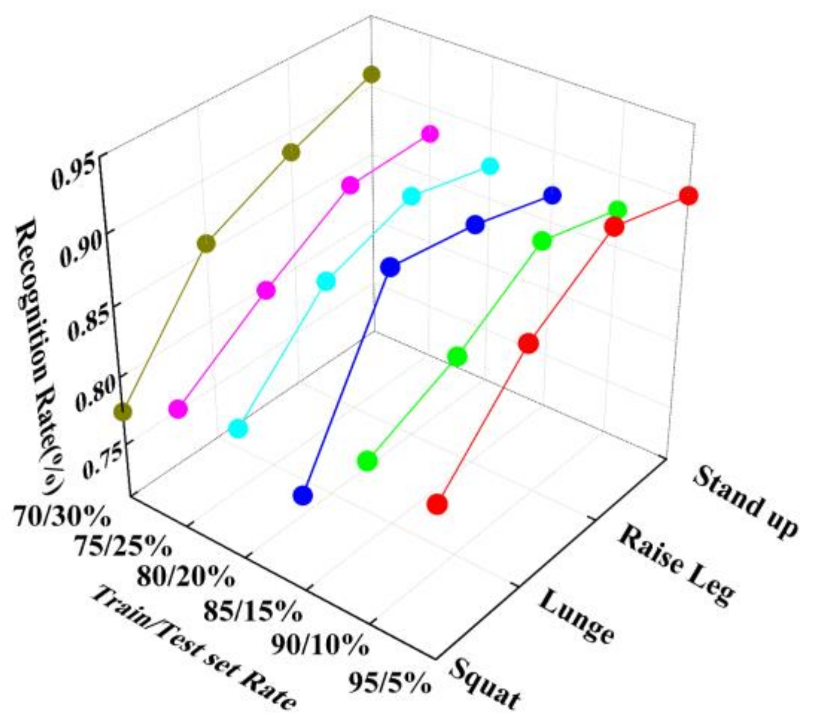
In the existing research on lower limb movement classification by EMG signals, when concluding the experiment, the methods used for selecting muscles are mostly based on the distribution position of human muscles or on the convenience of collection by researchers [12,13,14]. Although the results are still objective, they lack a certain scientific basis. Therefore, the contributions of this paper are summarized as follows. (1) We registered the changes in data of muscle length during gait movement according to OpenSim. To reduce the interaction and redundancy between various EMG signals, the principles of statistical mathematics and human anatomy are innovatively used to select those muscles with low correlation in the process of movement from numerous muscles of the lower limbs. (2) The correctness of muscle selection is verified by the use of a BP neural network. To make the results universal, we divided the proportions of the training set and test set into 95%/5%, 90%/10%, 85%/15%, 80%/20%, 75%/25%, and 70%/30%.

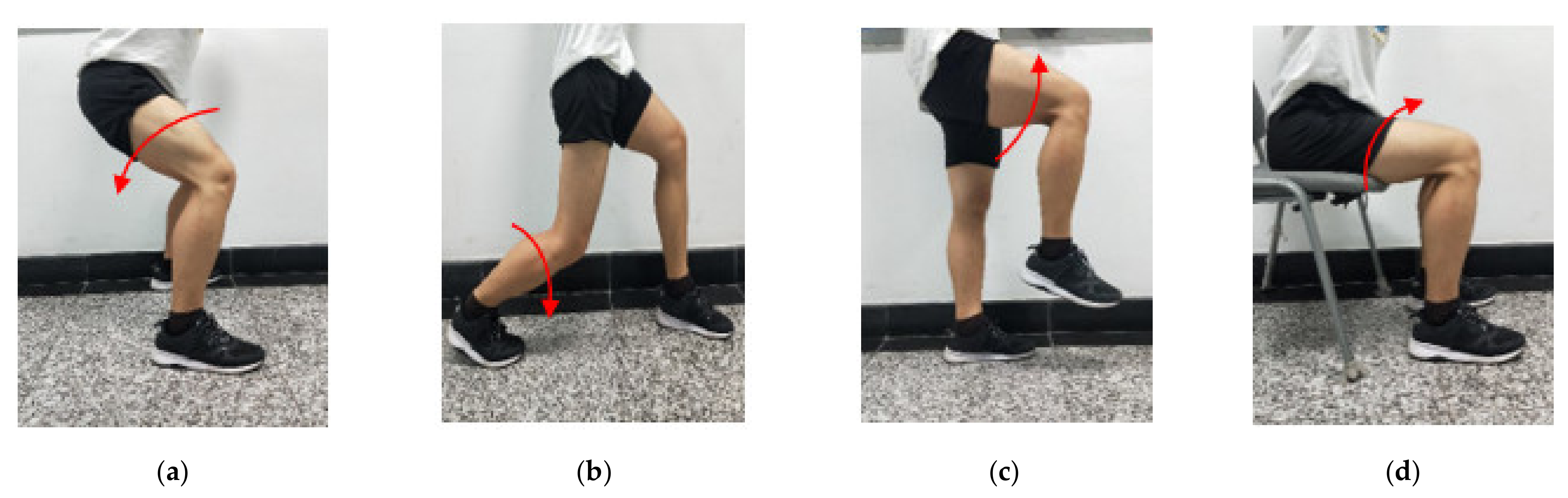
The road slopes, different gaits and lower limb movements selected in this paper are commonly found in work and life, and can be used for mutual verification of the muscle selection method and pattern recognition. The research results help to identify the states of movement of human beings and predict human movement intention, so as to achieve efficient and safe operation at work and at home.

2. Experiments and Methods

2.1. Research Objects and Test Parameters

We selected 10 healthy students (5 males and 5 females); their average age is 22.6 years (male) and 21.3 years (female); the average height is 175.59 cm (male) and 160.75 cm (female); the average weight is 74.86 kg (male) and 55.35 kg (female). All subjects had no motor dysfunction or congenital diseases, and all of them volunteered to participate in this research. Before the test, the volunteers did not undergo any strenuous exercise or suffer any fatigue, strain, or pain of lower limb muscles within the previous 24 h.

2.2. Angle Signal Measurement Method

The IMU sensor is tied onto the center of mass of the experimenter’s thigh and calf, to measure lower limb angle data in the sagittal plane. The value is the angle between the lower limb and vertical axis (thigh angle α and calf angle β). When the thigh and calf are perpendicular to the ground, angles α and β equal 0. When the thigh rotates counterclockwise relative to the hip joint, α is positive, and when the thigh rotates clockwise, α is negative. When the calf rotates counterclockwise relative to the knee joint, β is positive, and when the calf rotates clockwise, β is negative. A complete gait cycle is defined as: (a) bipedal standing (α = 0, β = 0); (b) lift the thigh, bend the knee and flex the calf (α > 0, β < 0); (c) extend knee into the gait support phase (α > 0, β > 0); (d) lift the thigh and bend the knee to flex the calf (α < 0, β < 0); (e) return to bipedal standing (α = 0, β = 0). Standing for the first time is defined as 0% in the gait cycle and standing a second time is defined as 100% in the gait cycle. The duration of the whole process is 2.5 s. The diagram mapping lower limb gait movement is shown in Figure 2.

2.3. EMG Signal Measurement Method

The periodicity of action of the lower limb determines the periodicity of muscle contraction. Movement of the ankle joint depends on calf muscle contraction, and the movement of the knee angle depends on thigh and calf muscle contraction. Therefore, selecting the right muscle and collecting its micro-EMG signal can reflect the macro movement of the lower limbs. However, due to the distribution of muscle positions (the EMG signal of deep muscles cannot be obtained) and the function of the muscle itself, we cannot obtain all muscle EMG signals. It is also unrealistic and unnecessary (excessive multi-dimensional EMG signals will cause signal redundancy and also become a burden for the classifier). Simultaneously, according to the principles of human anatomy and lower limb kinematics, there is a situation whereby the same action is completed by multiple muscle contractions. For example, the lateral femoral, medial femoral and rectus femoral muscle serve the same function in knee extension, the length of the muscle changes together with the angle of the knee joint [12]. In theory, their EMG signals also have a certain correlation.

Therefore, in order to select the appropriate muscles from which to collect EMG signals and optimize the original data, we chose 10 muscles related to gait movement according to muscle structure and distribution. They are the biceps femoris, the lateral head of the gastrocnemius, the medial head of the gastrocnemius, the rectus femoris, the sartorius muscle, semitendinosus, the tensor fascia lata, the tibialis anterior muscle, the lateral femoral muscle, and the medial femoral muscle. OpenSim (a form of musculoskeletal analysis software) was used to simulate the changes of those muscles in the process of gait movement. The selected human model, gait 2392_Simbody.osim, involves 19 bones and 92 muscles, and its height and weight are set at 1.8 m and 75 kg, respectively, giving us the data of muscle length change in the process of gait motion. To analyze the correlation among data of each muscle length and to decide which muscles could be selected to test the EMG signal, the correlation analysis module in SPSS (a statistical analysis software) was used in this paper. The parameter of PEARSON in the SPSS program was chosen as the correlation coefficient, and TWOTAIL NOSIG was selected for the significance test. The p-value shows the significant index, p > 0.05 indicates that the two variables are not related and are not significant; 0.01 < p < 0.05 is significant, whereas p < 0.01 is extremely significant. R is the correlation coefficient, and a negative R-value indicates a negative correlation, while a positive R-value indicates a positive correlation. The results are given in

Table 1. Correlation between lower limb muscles.

	Bi_fem		Lat_gas		Med_gas		Rec_fem		Sar
	R	P	R	P	R	P	R	P	R	P
Bi_fem	1		0.325	0.02	0.328	0.019	−0.934	0.000	−0.643	0.000
Lat_gas			1		1.000	0.000	−0.620	0.000	0.449	0.001
Med_gas					1		−0.623	0.000	0.449	0.001
Rec_fem							1		0.333	0.017
Sar									1

and

Table 2. Correlation between lower limb muscles.

	Sem		Tfl		Tib		Lat_fem		Med_fem
	R	P	R	P	R	P	R	P	R	P
Bi_fem	−0.988	0.000	−0.892	0.000	−0.056	0.698	−0.470	0.001	−0.468	0.001
Lat_gas	0.452	0.001	0.111	0.436	−0.882	0.000	−0.928	0.000	−0.928	0.000
Med_gas	0.455	0.001	0.109	0.445	−0.879	0.000	−0.930	0.000	−0.931	0.000
Rec_fem	−0.977	0.000	0.682	0.000	0.308	0.028	0.754	0.000	0.753	0.000
Sar	−0.524	0.000	0.909	0.000	−0.482	0.000	−0.366	0.008	−0.367	0.008
Sem	1		−0.820	0.000	−0.159	0.265	−0.596	0.000	−0.595	0.000
Tfl			1		−0.304	0.030	0.042	0.770	0.041	0.775
Tib					1		0.643	0.000	0.644	0.000
Lat_fem							1		1.000	0.000
Med_fem									1

.

According to the principles of mathematical statistics, if there is a high positive correlation between muscles, this indicates that the length of the two muscles tends to be consistent in the gait process; that is, the role of the two muscles in the flexion and extension of the joint is the same [13]. For example, in terms of the lateral femoral muscle and the medial femoral muscle, their function is to extend the knee, and their position on the thigh is similar, thus their correlation is 1, as with the lateral head and medial head of the gastrocnemius. The highly negative correlation between the muscles indicates that the length changes of the two muscles tend to be opposite in gait motion, that is, they play opposite roles in joint flexion and extension [13]. For example, the anterior tibialis and gastrocnemius are used for plantar and dorsal flexion of the ankle, so their correlation was −0.879.

According to the above analysis, in order to avoid data redundancy and repeatedly collect the EMG signals of muscles with the same function, we selected unrelated muscles from Table 1 and Table 2 above, which are the biceps femoris (knee flexion), the rectus femoris (knee extension), the lateral head of the gastrocnemius (knee flexion and plantar flexion), and the tibialis anterior muscle (dorsiflexion). The position of muscles in the lower limb of the volunteer is shown in Figure 3. The muscle surface has been cleaned by removing the hair and using a 70% concentration of alcohol to reduce EMG signal errors. The EMG sensor’s positive and negative electrodes were attached along the long axis of the muscle. Each volunteer walked on the experimental platform, keeping a standard gait; meanwhile, the EMG signals of the tested muscles were collected by an EMG signal measurement system (BIO-8). The test interval between each group of EMG signals was 30 min to ensure that the volunteers rested enough that their muscles could be fully relaxed.

EMG signals can be extracted and used for recognition, then they can help to control an exoskeleton or prosthesis [14,15]. However, excessive noise in the EMG signals will adversely affect the recognition rate. Therefore, it is critical to perform denoising. The noise is principally caused by power frequency interference during the acquisition process, and poor contact between the electrodes and the body surface will also result in the generation of noise [16]. According to the general characteristics of EMG signal noise, the Butterworth filter was adopted to denoise the signals. The frequency spectrum for EMG signals is primarily distributed in a range of 20 to 500 Hz [17]. Therefore, we used the Butterworth bandpass filter to filter out all noise except signals in the same frequency range. Then, a 50 Hz Butterworth notch filter was designed to filter the power frequency interference. Finally, the baseline drift signals were removed by an elliptic filter.

Then, the signals were extracted in time and frequency domains. Time-domain features included iEMG, RMS, and VAR. Frequency domain features included MF and MPF. The calculation formulas were as follows.

iEMG: This parameter reflects the muscle activity state in real-time and reflected muscle contraction characteristics in unit time [18].

$$iEMG={\displaystyle \underset{t}{\overset{t+T}{\int }}\left|EMG(t)\right|dt}$$

(1)

where t is time and EMG (t) is the voltage of EMG signal, T is the time window.

RMS: Changes in this parameter primarily reflect the number of motor units activated during muscle action, the types of motor units involved, and the degree of synchronization [18].

$$RMS=\sqrt{\frac{{\displaystyle \sum _{i=1}^N{X}_i^2}}{N}}=\sqrt{\frac{X_1^2+X_2^2+\dots +X_N^2}{N}}$$

(2)

where X_i is the voltage of EMG signal and N is the number of data in a signal time window.

VAR: This value reflects the variance in the EMG signals [18].

$$VAR=\frac{1}{N-1}{\displaystyle \sum _{i=1}^N{(X_i-\overline{X})}^2}$$

(3)

where X_i is the voltage of EMG signal and N is the number of data in a signal time window. $\overline{X}$ is the average value of EMG signal voltage in the time window.

Mean Power Frequency (MPF): At a certain point in time, the results included the fast Fourier transformation for all the active EMG signals power spectrum, and the frequency values corresponding to the average value of power [18]:

$$f_{mean}={\displaystyle {\int }_0^{+\infty }fP(f)}df/{\displaystyle {\int }_0^{+\infty }P(f)}df$$

(4)

where $P(f)$ represents the power spectral density function and f is the frequency of EMG signal.

Median Frequency (MF): This parameter was the point on the power spectrum where the energy on the left and right sides were equal [18]:

$${\displaystyle {\int }_0^{f_{mf}}P(f)}df={\displaystyle {\int }_{f_{mf}}^{+\infty }P(f)}df=\frac{1}{2}{\displaystyle {\int }_0^{+\infty }P(f)}df$$

(5)

where $f_{mf}$ represents the median frequency to be determined and $P(f)$ represents the power spectral density function.

The acquisition frequency of the EMG signal is 2000 Hz/s, and the acquisition time of each action/gait is 60 s, so each action/gait has 120,000 data points. The window size of each feature is 10 ms; that is, one eigenvalue is calculated for every 20 pieces of raw data; the size of the sliding window is 10 ms, which is calculated every 10 ms. Therefore, 6000 eigenvalues are reserved for each action/gait and are put to use as the input of the BP neural network.

2.4. Pattern Recognition Algorithm

The BP neural network, one of the most classic classifiers, adopts the learning algorithm of error backpropagation. Its outstanding advantages are a strong nonlinear mapping ability and flexible network structure [19]. Any continuous function in the closed interval can be approximated by the BP neural network with a single hidden layer, so a 3-layer BP neural network can complete the mapping from the N-dimension to the M-dimension. However, in order to achieve the expected mapping effect and to verify the ability of the EMG signal to reflect the lower-limb movement in each case, we chose a double hidden-layer BP neural network as the classifier of lower-limb movement. Its structure diagram is shown in Figure 4. The input of the BP neural network is the eigenvalue matrix of the EMG signal, and the output is the various gaits or actions. The BP neural network used in this paper has 1 input layer, 2 hidden layers and 1 output layer. The number of input layer nodes is 20 (20 eigenvalues of 4 muscles), and the number of hidden-layer nodes is 15. The output layer changes according to the needs of the classification process. The specific values are described in the following sections. The learning rate was set to 0.001, the epoch was set to 100, and the training goal was set to 0.00004. After the above data processing was completed, each action or gait retained 6000 groups of EMG signal data.

In this paper, the purpose of using the classifier to identify the movements of lower limbs is to verify the correctness of the muscles selected by the SPSS statistical mathematics method and human anatomy principles. Thus, the BP neural network is only a classification tool; the focus is not to prove that BP is inherently superior to other classifiers. Simultaneously, in order to make the results universal, we divided the proportions of the training set and test set into 95%/5%, 90%/10%, 85%/15%, 80%/20%, 75%/25%, and 70%/30%. Therefore, this paper does not compare the BP network with other classification algorithms. Finally, this research was funded by the Aerospace Research Project of China. The research aim of the project is to enhance the abilities of normal people, not to be involved in the field of rehabilitation medicine. Therefore, there were no comparisons made between able and disabled people.

3. Analysis and Recognition

3.1. Recognition of Road Gradient Based on EMG Signals

To study the influence of slope on the angle of the lower limb and the EMG signal, 7 different slopes were simulated via a treadmill to complete the walking gait; the slopes were –15%, −10%, −5%, 0%, 5%, 10%, and 15%. According to the method of measuring the angle signal above, we established the angles of the thigh and calf at different slopes in a single gait cycle, which is shown in Figure 5. It can be seen that the thigh angles on different slopes are basically the same. There are two peaks of the thigh angle through the whole gait cycle, and the first peak is higher. The first peak occurs at 20% of the gait cycle, which is the initial stage of the supporting phase. The extreme angle of the thigh increases as the road slope increases, from −15% to 15%. However, there was no significant difference in the second peak, which appears at 80% of the gait cycle. The thigh angles on different slopes are basically the same except for the slope of 15%. The first minimum of the calf angle appeared earlier than that of the thigh, at about 3% of the gait cycle. There is one situation where the calf angle remains unchanged, at 40–60% when the road slope reaches more than 10%. It is also demonstrated in Figure 5 that when the road slope tends to be gentle, the first maximum value of the calf angle is larger. The flat ground is the largest value, which is about 20° higher than the maximum slope.

Therefore, the difference in slope is mainly reflected in the first peak of the thigh angle. There is a positive linear correlation between the slope and the peak angle of the thigh. This is determined by the gait characteristics. The peak of the thigh angle appears at the beginning of the support phase; when the foot touches the ground, the thigh angle reaches the maximum, then decreases. Figure 6 illustrates the thigh angle α of the test leg under different slopes during gait movement. The following conclusions can be drawn from Figure 6: when the slope increases, the center of gravity of the calf and foot becomes higher at the beginning of the support phase, which makes the thigh rotate more counterclockwise around the hip joint.

According to the above analysis, there are slight differences in the angle of the lower limbs on different slopes. In order to explore the feasibility of using the EMG signal to identify road slope. In this paper, the EMG signals of the lower limbs of the test subjects, walking on different slopes, were collected via the BIO-8 system (equipment for collecting EMG signals). The EMG signals from three gait cycles are shown in Figure 7.

Figure 7 illustrates the EMG signals of the 4 muscles of the lower limbs when the test subject walks on 7 different slopes. It can be seen from the figures that the EMG signals of the selected muscles change periodically during walking, and each cycle has a certain separability. The EMG signal of the biceps femoris is the strongest, and the amplitude is up to above ±10 mV. The amplitude of the gastrocnemius EMG signal becomes larger with the slope increasing from −15% to 15%. After filtering results of feature extraction, the EMG signals are constructed into a 20-dimensional feature matrix, which is used as the input of a double hidden-layer BP neural network to identify 7 different slopes. The number of input layer nodes is 20, the number of hidden layer nodes is 15, and the number of output layer nodes is 7. Taking 95%, 90%, 85%, 80%, 75% and 70% of the total data as the training set of the BP neural network, and taking 5%, 10%, 15%, 20%, 25% and 30% of the total data as the test set of the BP neural network to identify the feasibility of recognizing the slope of the ramp by the EMG signal. The recognition results are shown in Figure 8.

As can be seen in Figure 8, the double hidden-layer BP neural network has a good recognition effect according to the slope.

Table 3. Recognition rate in 7 slopes under different test set/verification set ratios.

Training/Test Set Rate	95%/5%	90%/10%	85%/15%	80%/20%	75%/25%	70%/30%
Average Recognition Rate	0.8680	0.8704	0.8587	0.8653	0.8728	0.8537

indicates the average recognition rate of each training/test set for 7 kinds of gait. The recognition rate of the slope of the test set/verification set at various proportions is above 85%, which means that the EMG signal of lower-limb muscles can achieve the effect of identifying the slope of the ramp.

The division ratio of the training set and test set of the EMG data is set at 70%/30%, and the BP neural network is iteratively trained. The error curve is shown in Figure 9. It shows that when the number of iterations reaches 40, the iterative error of the BP neural network tends to be stable and fluctuates within a certain value.

The average recognition rate of the BP neural network for 7 kinds of slope is shown in

Table 4. Average recognition rates in 7 slopes of the BP neural network.

Slope	−15%	−10%	−5%	0%	5%	10%	15%	Average
Average Recognition Rate	0.7925	0.8867	0.923	0.8827	0.8526	0.7988	0.9175	0.8649

. The recognition rate of the BP neural network for −15% and 10% is low and is only 0.79. But the recognition rate for 15% is above 0.91. The recognition rates of slopes with gradients of −5% and 15% are 0.923 and 0.9175, respectively.

3.2. Recognition of Gait Based on EMG Signal

In order to ensure that the slope of the ramp and the step are the same, the selected test site is arranged as shown in Figure 10. There are 12 steps in the flight of stairs in total, the height is 0.15 m, the width is 0.40 m, the length of the step is 3 m, and the vertical height at the last step is 1.8 m. The slope of the step (the included angle between the line of each leading edge of each step and the horizontal plane) is 37.5%. The ramp is built on both sides of the step to ensure that the gradient of the step and the ramp are the same, so the slope gradient is also 37.5%. Marked points on the slope, according to the corresponding position of the step, ensure the same stride of the tester when walking on either the step or the slope. The specific parameters of the flat test site are as follows: selecting a spacious and barrier-free flat area and marking points in the test site to ensure the same stride length (0.42 m) according to the parameters of the slope and step.

According to the gait database curve, the lower-limb joint angle changes periodically during the natural human walking gait cycle [20]. Specifically, the lower limb joint angle is variable when walking on different course surfaces. However, the changes of limb and joint angles during exercise have not been clearly studied. At the same time, the recognition of human motion states based on the angle of the lower limbs needs further research.

Based on these findings, IMU sensors were attached to the center of mass of the thigh, leg and instep of the test subject to measure the kinematic parameters of the lower limbs in the sagittal plane during various gait processes. The 3 road conditions are set at flat, a ramp and steps, so the 5 gait types are walking on flat ground, uphill, downhill, up steps and down steps. Figure 11 expresses the angle signals of the thigh and calf in a single gait cycle. In Figure 11a, when the cycle is at 20%, the angle of the thigh reaches the maximum value, and the angle of the thigh in the upward step is the greatest (65°), followed by uphill (58°), and the last three are almost the same. When the gait cycle is 65%, the angle of the thigh reaches the lowest value, and the angle of downward step and downhill is smaller than the other three. When the gait cycle reached 85%, the thigh angle reached the maximum value for the second time, and the down-step gait was the largest (35°), while the flat gait was the lowest (0°).

Figure 11b depicts the calf angle of different gaits. When the cycle is 15%, the calf angle reaches the maximum value for the first time, and the angle of the upward step is the largest (33°), followed by the angle of uphill (25°), and the other 3 gaits are the same; then, the calf angle decreases. When the gait period is 25%, it reaches the minimum for the first time. Simultaneously, the angle uphill and up the step is obviously larger than for the other three. When the gait cycle is at 80%, the calf angle reaches the minimum value for the second time. Simultaneously, the angle values, ranging from smallest to largest, are downward step, downhill, upward step, flat ground and uphill, respectively, but the angle difference between each gait is relatively small.

The EMG signal acquisition test was carried out on the test site in Figure 12, and the signal of each gait was collected for 60 s. Each gait type is extracted according to the characteristics of the signal, of which three cycles are set as the research objects, and the results are shown in Figure 12a–e. It can be seen that the waveform of the lower-limb EMG signal is different and presents a different periodicity in each different gait, and the same muscle in each different gait showed different periodic strength. When walking on the flat ground, the signals of the rectus femoris, biceps femoris and anterior tibialis have strong periodicity. The signal range of the rectus femoris is −6.5–6.0 mV, the signal range of the biceps femoris is 0.5–2 mV, and the signal range of the anterior tibialis is −11.5–10.5 mV. There is no obvious periodicity of the gastrocnemius muscle because the ankle angle does not change significantly when walking on flat ground, so the periodicity of the gastrocnemius muscle EMG signal is poor. The signal intensity of the rectus femoris when moving uphill was stronger than that in the flat gait, whose range is from −9.5–8.5 mV. The periodicity of the EMG signal of the biceps femoris is weak in this gait. The EMG signals of the tibialis anterior muscle and gastrocnemius muscle of the calf are periodically weak when walking downhill. The EMG waveform of the rectus femoris was similar to that of walking on flat ground. The periodicity of the biceps femoris and anterior tibialis were stronger when walking up steps and down steps.

The lower limb angles of 5 different gaits under 3 different surface conditions are similar but there are still some differences. Based on this finding, we collected the EMG signals of lower limbs in 5 kinds of gait and used those EMG signals as the input of the double hidden-layer BP neural network to identify 5 kinds of gait. The number of nodes in the input layer of the BP neural network is 20 (a 20-dimensional characteristic matrix of 4 muscles), the number of nodes in the hidden layer is 15, and the number of nodes in the output layer is 5 (5 kinds of gait). The results are shown in Figure 13.

Table 5. The recognition rates of 5 gaits under different test set/verification set ratios.

Test/Verification Set Ratio	95%/5%	90%/10%	85%/15%	80%/20%	75%/25%	70%/30%
Average Recognition Rate	0.9331	0.9383	0.9435	0.9393	0.9366	0.9344

shows the average recognition rate of the double hidden-layer neural network for 5 kinds of gait under different training set/test set ratios. As seen in Table 5, the double hidden-layer BP neural network has a good recognition effect for different gaits, and the recognition rate of the slope of the test set/verification set at various proportions is above 93%, which is better than that based on the EMG signal for recognizing 7 kinds of slope. The reason for this is that the discrimination of 5 movements is greater than that of 7 slopes, and the periodicity of the EMG signals of five movements is more obvious so the recognition rate is higher.

Similarly, the data set was divided up in the proportion of 70%/30%, and the training curve of the BP neural network is as follows. Figure 14 shows the training curves of the BP neural network for 5 gait types. The horizontal ordinate is the number of iterations (from 0 to 100), and the longitudinal coordinates are the recognition error. It can be seen from Figure 14 that when the number of iterations reaches 18, the recognition error of the double hidden-layer BP neural network for 5 gait types tends to be a stable value, and the convergence speed of the BP neural network is fast. This shows that the EMG signals of the rectus femoris, biceps femoris, anterior tibial muscle and gastrocnemius muscle can typify different gaits.

The average recognition rate of the BP neural network for 5 different kinds of gait is shown in

Table 6. Average recognition rate in 5 gaits of the BP neural network.

Gait	Flat Ground	Uphill	Downhill	Up Step	Down Step	Average
Average Recognition Rate	0.9429	0.9075	0.9224	0.9228	0.9923	0.9376

. The recognition rate of the double hidden-layer BP neural network is 0.9923 for the downward step, 0.9429 for the flat ground, and 0.9075 for uphill movement. From the above analysis of lower-limb angles in different gaits, it can be seen that the joint angles of lower limbs are quite different in the 5 different gaits. Therefore, there is a difference in the contractions of the lower limb muscles and their EMG signals [21]. Thus, the recognition rate of the BP neural network for the 5 kinds of gait is higher. The average recognition rate was 0.9376, which was higher than that of the BP neural network for 7 slopes (0.8649).

3.3. Recognition of Movement Based on the EMG Signal

In this section, we explore the similarities and differences in the EMG signals of lower limb muscles. The joint movements of knee flexion and extension are the same but the lower limb movements are different, and the feasibility of identifying different movements with EMG signals is also discussed in this case. We selected 4 common movements, which are:

Squatting (feet shoulder-width apart. The thigh rotates counterclockwise around the knee joint to make the center of gravity move down and then reset, which is a squat cycle. The position of the knee joint remains unchanged during the movement).

Lunging (stand with both feet forward and backward, rotate the calf clockwise around the knee joint to make the center of gravity move down and then reset, which is a lunge cycle. During the movement, the position of the knee joint first decreases and then increases with the movement).

Raising the leg (the thigh rotates anticlockwise around the hip joint horizontally and then resets, which is a raised leg cycle; the body’s center of gravity remains unchanged, the knee joint first rises and then drops with the rotation of the thigh during the movement).

Standing up (from standing, down to sitting on the chair, and then standing up forms a standing-up cycle; the position of the knee joint remains unchanged during the movement.) The schematic diagram of the 4 actions is shown in Figure 15.

The figures below indicate the angle changes of the thigh and calf in a movement cycle. As can be seen from Figure 16a,b, the 4 movements are mainly the change of thigh angle. Their change trend is the same but there is some difference at the maximum value; the highest is in the raise leg movement (107°), the second is stand up (98°), the third is squat (76°), and the lowest is the lunge (61°). There was no obvious regularity in the changes of calf angle; only the lunge had the largest range (−53°).

It is required that the subject completes the specified action within 2 s and repeats it after 2 s. Therefore, a total of 15 motion cycles were collected in the sampling period of 60 s. The results are shown in Figure 17a–d. The EMG signals of each muscle of the lower limbs during each action suggest good periodicity, and the active state and the resting state of the signals have a good distinction. The same muscle shows different EMG signal waveforms during different actions. When squatting, the EMG signal of the gastrocnemius muscle is weak, when lunging, the rectus femoris muscle has a strong signal in the resting state, which leads to the weak periodicity of the signal. The signal amplitude of the tibialis anterior muscle and gastrocnemius muscle on the calf was smaller when raising the leg and standing up. This is because these two movements are mainly completed via the active movement of the thigh [22]. As seen in Figure 17b, there is no certain regularity in the angle change of the calf during the two movements.

After noise reduction and feature extraction, the EMG signals of these 4 movements are used for input in the double hidden-layer BP neural network. The number of nodes in the input layer of the BP neural network is 20 (20-dimensional characteristic matrix of 4 muscles), the number of nodes in the hidden layer is 15, and the number of nodes in the output layer is 4 (4 kinds of movement). The results are shown in Figure 18. The recognition rate of the BP neural network for the 4 movements is low, but it still remains above 0.75 (squatting). When the proportion of the training set/test set reaches 95%/5%, the recognition rate of the BP neural network for squatting is the lowest (0.7747). When the proportion of the training set/test set reaches 70%/30%, the recognition rate of the BP neural network for standing movements is the highest, reaching 0.9185.

Table 7. Recognition rate in 4 movements under different test set/verification set ratios.

Training/Test Set Ratio	95%/5%	90%/10%	85%/15%	80%/20%	75%/25%	70%/30%
Average Recognition Rate	0.8809	0.8620	0.8571	0.8581	0.8496	0.8562

shows the average recognition rate of the double hidden-layer BP neural network for 4 kinds of movement under different training set/test set ratios. As can be seen, the double hidden-layer BP neural network has a good recognition effect for different movements and the recognition rate at various proportions is above 0.84.

The dataset was divided in the proportion of 70%/30%, and the training curve of the BP neural network for 4 movements is as follows (Figure 19). It demonstrates that the training curves of the BP neural network for 4 movements converge faster.

Table 8. Average recognition rate in 4 movements of the BP neural network for the ramp.

Movements	Squat	Lunge	Raise Leg	Stand Up	Average
Average Recognition Rate	0.801	0.8653	0.8911	0.8853	0.8607

shows the average recognition rate of each action in different training set/test set proportions. The recognition rate is 0.801 for the squat, 0.8653 for the lunge, 0.8911 for raising the leg, and 0.8853 for standing up. The average recognition rate was 0.8607, which was lower than that of the BP neural network for 5 gaits (0.9376), and almost equal to that of the BP neural network for 7 slopes (0.8649).

4. Discussions

Sensors are now the eyes and ears of automatic control. When they are applied to the human body, we hope that the sensor has the same perception ability as the human sensory organ it mimics. Sensors have the ability to detect the potential human perception of the external environment, such as vision, force, touch, smell and taste inside the human body or on the human surface [5,6,7], which has gradually become an indispensable part of the control system when wearing robot or intelligent prostheses. With the development of human motion intention recognition technology, soft and comfortable EMG sensors stand out among the many forms of human motion signal sensors. Surface EMG signals also offer various excellent properties and are well known by researchers.

Through the evolution of human beings, lower limb muscles are numerous and more developed. Each muscle performs its own duties in the process of exercise and also emits various EMG signals. However, which EMG signal from which muscle is more representative has not yet seen a mature method of assessment and conclusion. Methods of selecting muscles are mostly based on the distribution position of human muscles or on the convenience of collection for testers when finishing an experiment. Therefore, to solve this problem, the change data of muscle length during gait was simulated according to OpenSim in this article; several principles of statistical mathematics and human anatomy analysis are innovatively used to select muscles from the numerous muscles of the lower limbs for the first time. Four muscles in the lower limb with a low correlation through gait were selected via OpenSim and the SPSS correlation analysis module. These muscles are proven to reduce the interaction and redundancy between various EMG signals. To test this conclusion, a BP neural network with a double hidden layer was utilized at different proportions of the training set and test set. After denoising with a Butterworth filter and feature extraction in the time and frequency domain, EMG signals were used as the input of the BP neural network to recognize various gaits/movements. The road slopes, different gaits and lower limb movements selected in this paper are common in work and life and can be used in the mutual verification of muscle selection methods and pattern recognition. To make the results universal, we divided the proportions of the training set and test set into 95%/5%, 90%/10%, 85%/15%, 80%/20%, 75%/25%, 70%/30%. The results indicate that the muscles with a low correlation in the lower limbs can be distinguished by statistical principles. Taking the selected four muscles as the input for the recognizer, different road slopes, road conditions and lower limb movements can also be typified, which shows a better recognition result than other signal-based methods [23,24,25,26]. The research results help to identify the movement states of humans and predict human movement intention, so as to achieve efficient and safe operation.

5. Conclusions

In this paper, four muscles in the lower limb with a low correlation through gait were selected by the OpenSim and SPSS correlation analysis module. The lower limb angle and EMG signals were collected for seven slopes, five gaits and four movements through experiments. After denoising with a Butterworth filter and feature extraction in the time and frequency domain, EMG signals were used as the input of a BP neural network to recognize various gaits/movements. The conclusions are as follows:

(1)

With the increase of slope, the thigh angle peak increases, but there is no obvious difference in the changes of calf angle. The periodicity of the EMG signal of these four muscles is obvious. The BP neural network recognition rate of seven kinds of slope were 0.7925, 0.8867, 0.923, 0.8827, 0.8526, 0.7988, and 0.9175, which shows that the EMG signals of muscles selected by correlation analysis can identify various road slopes.

(2)

Different gaits had significant effects on the angles of the thigh and calf, and the maximum angle of the thigh was 65° and 58° when walking uphill and up steps. The minimum value of the calf was −48° and −58° when walking downhill and up steps. The EMG signal had good periodicity and it shows different waveforms in different gaits. Moreover, the periodicity of the gastrocnemius muscle is weak when walking downhill and up steps. The recognition effect of the BP neural network for five gaits is better than that for seven slopes, and the recognition rate for the gait of the downward step was the best, reaching 0.9923. The average recognition rate also reached 0.9376, which means that the EMG signals of muscles selected by correlation analysis can identify different gaits.

(3)

Four movements (squats, lunges, raising a leg and standing up) that were the same as in knee rotation, but where the muscles work in different ways, were selected. The study found that the thigh angle in each instance was basically the same, while the calf angle did not change regularly. The periodicity of the EMG signals in the gastrocnemius muscle was weak during the squat and the tibialis anterior muscle of the calf was weak during standing up. The recognition rates of the BP neural network for four movements were 0.801, 0.8653, 0.8911, and 0.8853, respectively, which illustrates that the EMG signals of muscles selected by correlation analysis can identify different movements of the lower limb.

References

1. Liu, L.; Yang, P.; Liu, J. Human Motion Intent Recognition Based on Kernel Principal Component Analysis and Relevance Vector Machine. Robot 2017, 5, 661–669. [Google Scholar]
2. Yang, Z.Z.; Wu, D.W.; Tao, J. Review and Prospect of Study on Energy Metabolism in Manned Space Flight. Manned Spacefl. 2016, 22, 655–662. [Google Scholar]
3. Xu, H.Q.; Liu, F.; Nan, J.W. Motion Research of Power-Assisted Lower Extremity Exoskeleton under Walking Process. Mach. Des. Manuf. 2019, 341, 107–110. [Google Scholar]
4. Wu, X.; Fang, K.; Chen, C.; Zhang, Y. Development of a lower limb multi-joint assistance soft exosuit. Sci. China Inf. Sci. 2020, 63, 1–3. [Google Scholar] [CrossRef]
5. Lu, D.M. Measurement Methods of Sports Biomechanics; Beijing Sport University Press: Beijing, China, 2001; pp. 65–71. [Google Scholar]
6. Li, Y.; Wang, L. Gait and face profile fusion based human identification at a distance in video. Chin. J. Sci. Instrum. 2011, 32, 264–270. [Google Scholar]
7. Zhang, K.; Luo, J.; Xiao, W.; Zhang, W.; Liu, H.; Zhu, J.; Rong, Y.; de Silva, C.W.; Fu, C. A Subvision System for Enhancing the Environmental Adaptability of the Powered Transfemoral Prosthesis. IEEE Trans. Cybern. 2020, 51, 3285–3297. [Google Scholar] [CrossRef] [PubMed]
8. Zhong, B.; da Silva, R.L.; Li, M.; Huang, H.; Lobaton, E. Environmental context prediction for lower limb prostheses with uncertainty quantification. IEEE Trans. Autom. Sci. Eng. 2020, 18, 458–470. [Google Scholar] [CrossRef]
9. Wan, D.; Zhang, L.; Bai, Y.; Xie, Y. Research on Identification Algorithm Based on ECG Signal and Improved Convolutional Neural Network. J. Phys. Conf. Ser. 2021, 1757, 012046. [Google Scholar] [CrossRef]
10. Laport, F.; Iglesia, D.; Dapena, A.; Castro, P.M.; Vazquez-Araujo, F.J. Proposals and Comparisons from One-Sensor EEG and EOG Human-Machine Interfaces. Sensors 2021, 21, 2220. [Google Scholar] [CrossRef]
11. Chowdhury, R.H.; Reaz, M.B.I.; Ali, M.A.B.M.; Bakar, A.A.A.; Chellappan, K.; Chang, T.G. Surface Electromyography Signal Processing and Classification Techniques. Sensors 2013, 13, 12431–12466. [Google Scholar] [CrossRef]
12. Li, Q.; Zhang, A.; Li, Z.; Wu, Y. Improvement of EMG Pattern Recognition Model Performance in Repeated Uses by Combining Feature Selection and Incremental Transfer Learning. Front. Neurorobot. 2021, 15, 699174. [Google Scholar]
13. Moreira, L.; Figueiredo, J.; Fonseca, P.; Vilas-Boas, J.P.; Santos, C.P. Lower limb kinematic, kinetic, and EMG data from young healthy humans during walking at controlled speeds. Sci. Data 2021, 8, 103. [Google Scholar] [CrossRef]
14. Rainoldi, A.; Melchiorri, G.; Caruso, I. A method for positioning electrodes during surface EMG recordings in lower limb muscles. J. Neurosci. Methods 2004, 134, 37–43. [Google Scholar] [CrossRef] [PubMed]
15. Rafiee, J.; Rafiee, M.A.; Yavari, F.; Schone, M.P. Feature extraction of forearm EMG signals for prosthetics. Expert Syst. Appl. Int. J. 2011, 38, 4058–4067. [Google Scholar] [CrossRef]
16. Bisi, S.; Luca, L.D.; Shrestha, B. Development of an EMG-Controlled Mobile Robot. Robotics 2018, 7, 36. [Google Scholar] [CrossRef] [Green Version]
17. Majid, M.S.H.; Khairunizam, W.; Shahriman, A.; Zunaidi, I.; Sahyudi, B.N.; Zuradzman, M. EMG Feature Extractions for Upper-Limb Functional Movement During Rehabilitation. In Proceedings of the 2018 International Conference on Intelligent Informatics and Biomedical Sciences (ICIIBMS), Bangkok, Thailand, 21–24 October 2018; pp. 314–320. [Google Scholar]
18. Liu, D.R.; Paweł, B. Influence of type of MVC test on electromyography measures of biceps brachii and triceps brachii. Int. J. Occup. Saf. Ergon. 2018, 24, 200–206. [Google Scholar]
19. Omari, F.A.; Hui, J.; Mei, C.; Liu, G. Pattern Recognition of Eight Hand Motions Using Feature Extraction of Forearm EMG Signal. Proc. Natl. Acad. Sci. USA 2014, 84, 473–480. [Google Scholar] [CrossRef]
20. Zhang, L. An upper limb movement estimation from electromyography by using BP neural network. Biomed. Signal Process. Control 2019, 49, 434–439. [Google Scholar] [CrossRef]
21. Allen, D.G.; Lamb, G.D.; Westerblad, H. Skeletal muscle fatigue: Cellular mechanisms. Physiol. Rev. 2008, 88, 287–332. [Google Scholar] [CrossRef] [Green Version]
22. Wankhade, P.S.; Rajani, R. A Study of Various Methods for Detection and Analysis of EMG Signal and Its Application. Iosr J. Electron. Commun. Eng. 2019, 14, 48–54. [Google Scholar]
23. Tomasevicz, C.L.; Woldstad, J.C.; Jones, D.D. Risk of injury analysis in depth jump and squat jump. J. Hum. Sport Exerc. 2021, 17. [Google Scholar] [CrossRef]
24. Rezazadeh, S.; Quintero, D.; Divekar, N.; Reznick, E.; Gray, L.; Gregg, R.D. A Phase Variable Approach for Improved Rhythmic and Non-Rhythmic Control of a Powered Knee-Ankle Prosthesis. IEEE Access 2018, 7, 109840–109855. [Google Scholar] [CrossRef] [PubMed]
25. Madgwick, S.O.H.; Harrison, A.J.L.; Vaidyanathan, R. Estimation of IMU and MARG orientation using a gradient descent algorithm. In Proceedings of the 2011 IEEE International Conference on Rehabilitation Robotics, Zurich, Switzerland, 29 June–1 July 2011; pp. 1–7. [Google Scholar]
26. Liu, L.; Jiao, Y.; Meng, F. Key Algorithm for Human Motion Recognition in Virtual Reality Video Sequences Based on Hidden Markov Model. IEEE Access 2020, 8, 159705–159717. [Google Scholar] [CrossRef]
Figure 1. Research process in this paper.
Electronics 10 02473 g001
Figure 2. Relative position model of lower limb. (a) α = 0, β = 0; (b) α > 0, β < 0; (c) α > 0, β > 0; (d) α < 0, β < 0; (e) α = 0, β = 0.
Electronics 10 02473 g002
Figure 3. Position of selected muscles and reference electrodes: (a) front side; (b) back side.
Electronics 10 02473 g003
Figure 4. Double hidden-layer BP network structure diagram.
Electronics 10 02473 g004
Figure 5. Angle of the lower limb on different slopes. (a) Thigh angle on different slopes; (b) calf angle under different slopes.
Electronics 10 02473 g005
Figure 6. The ultimate angle of the thigh on different slopes.
Electronics 10 02473 g006
Figure 7. EMG signal of the lower limb in 7 slopes. (a) EMG signal of the rectus femoris; (b) EMG signal of the biceps femoris; (c) EMG signal of the tibialis anterior muscle; (d) EMG signal of the gastrocnemius.
Electronics 10 02473 g007
Figure 8. The recognition rate of lower-limb EMG signal according to the slope.
Electronics 10 02473 g008
Figure 9. Training curves of the BP neural network for 7 slopes.
Electronics 10 02473 g009
Figure 10. Test site for steps and ramps.
Electronics 10 02473 g010
Figure 11. Angle of the lower limb in different gaits. (a) Thigh angle in different gaits; (b) calf angle in different gaits.
Electronics 10 02473 g011
Figure 12. EMG of lower limb in different gait. (a) Flat ground; (b) uphill; (c) downhill; (d) squat; (e) side squat.
Electronics 10 02473 g012
Figure 13. The recognition rate of the lower limb EMG signal according to gait.
Electronics 10 02473 g013
Figure 14. Training curves of the BP neural network for 5 gait types.
Electronics 10 02473 g014
Figure 15. Four movements of the lower limb. (a) Squatting; (b) lunging; (c) raising the leg; (d) standing up.
Electronics 10 02473 g015
Figure 16. Changes of lower limb angle in 4 movements. (a) Thigh angle; (b) calf angle.
Electronics 10 02473 g016
Figure 17. EMG of the lower limb in different movement. (a) Squatting; (b) lunging; (c) raising the leg; (d) standing up.
Electronics 10 02473 g017
Figure 18. The recognition rate of lower-limb EMG signal to movements.
Electronics 10 02473 g018
Figure 19. Training curves of the BP neural network for 4 movements.
Electronics 10 02473 g019