Multi-Connectivity Enhanced Communication-Incentive Distributed Computation Offloading in Vehicular Networks

Abstract

Flexible resource scheduling and network forecast are crucial functions to enhance mobile vehicular network performances. However, BaseStations (BSs) and their computing unit which undertake the functions cannot meet the delay requirement because of limited computation capability. Offloading the time-sensitive functions to User Equipment (UE) is believed to be an effective method to tackle this challenge. The disadvantage of the method is offloading occupies communication resources, which deteriorate the system capability. To better coordinate offloading and communication, a multi-connectivity enhanced joint scheduling scheme for distributed computation offloading and communication resources allocation in vehicular networks is proposed in this article. Computation tasks are divided into many slices and distributed to UEs to aggregate the computation capability. A communication-incentive mechanism is provided for involving UEs to compensate the loss of UEs, while multi-connectivity is adopted to enhance the system throughput. We also defined offloading failure ratio as a conclusive condition for offloading size by analyzing the movement of UEs. By a two-step optimization, the co-scheduling of offloading size and throughput is solved. The system-level simulation results show that the offloading size and throughput of the proposed scheme are larger than comparisons when the time constraint is tight.

1. Introduction

The mobile communication network has grown rapidly in the past few decades. Global mobile data traffic will reach 77.5 Exabytes per month in 2022, which will increase seven-fold in 5 years [1]. The Fifth-Generation Mobile Communication System (5G) operated in 2019 brings various new features to the network. Many requirements, including latency, reliability, and connection brought by new applications, are different from traditional traffic. New communication devices, such as vehicles, which can provide computation services, relay, and cache, bring enormous extensibilities to the networks. The explosion of network data, various requirements, and new types of devices not only are significant challenges but also great opportunities to the existing mobile networks. High-performance computation is regarded as one of the feasible ways to tackle these challenges and opportunities [2,3,4].

On the Radio Access Network (RAN) side, BSs use computation and machine learning to realize complex schedule algorithms and prepare communication resources in advance. However, the capability of BSs is not always powerful enough to do the computation. Clouds equipped with high-performance Central Processing Units (CPUs) are adopted to make up for the shortage [5]. Through high-speed fiber, BSs offload part of computation tasks to the cloud and retrieve the results after computing is accomplished. In this way, BSs realize flexible resource scheduling and network forecast to improve the system performance.

However, vehicular networks often serve time-sensitive traffic. Although the computation capability of the cloud is high, the signal spreading delay brought by the long physical distance between cloud and BSs cannot satisfy the time requirement of such traffic [6]. With the development of low-power CPUs, mobile computing devices, especially vehicles, have much more powerful computing capability than ever [7]. UEs surrounding BSs become another computation capacity resource. Although the computation capability is weak compared to cloud, the weakness of UE offloading over computation capability can be covered by distributed computation [8]. Additional, UE offloading has the ascendancy over cloud computing on delay because of the short distance between BSs and UEs.

Many works have been focused on computation offloading [9,10,11,12], but only a few works consider the effect of computation offloading on system throughput. In the situation that UEs process computation tasks from BSs, computation offloading helps BSs improve the capability of networks. Meanwhile, they consume the energy of UEs and occupy bandwidth initially used for communication, which decreases system throughput. Computation and communication which restrict and promote each other are tightly associated in the future networks. How to jointly schedule them is a great challenge.

Another important factor to influence the action of UEs in the computation offloading research is the movement of UE. When UEs move out of the offloading area of BSs, BSs cannot transmit offloading tasks to UEs, which means this part of offloading is failed. Some works researched mobility in the computation offloading problems [13,14,15]. However, the movement of UEs is considered to bejust one dimensional path along a straight line, which is too simple to reflect the real situation.

In this paper, we introduce a multi-connectivity enhanced joint scheduling scheme of distributed computation offloading and communication resource allocation in vehicular networks. The scheme aims to improve the utility combined by offloading size and system throughput. Computation tasks from BSs will be split and distributed to UEs, while bandwidth is used to reward UE for offloading. Movement analysis is adopted to restrict the offloading proportion, and multi-connectivity is adopted to enhance the system throughput. The main contributions of this article are summarized as follows.

(1) We propose a joint scheduling scheme for distributed computation offloading and communication resources allocation to improve system throughput in vehicular networks. The time-sensitive computation task that BSs cannot complete in time will be split into many pieces and distributed to UEs. The offloading size and throughput are considered to realize the joint scheduling, where multi-connectivity is adopted to enhance the throughput by translating strong interferences to useful signals.

(2) The communication resources are explored to stimulate UEs to participate in the offloading. To compensate and stimulate UE, UEs involving in the offloading will gain more bandwidth. The bandwidth rewards factor is decided by the offloading size and UE characters, including the tolerance factor and requirement factor. Computation offloading and communication are associated as Multi-connectivity enhanced Communication-incentive Distributed Computation (MCDC) in the system.

(3) We analyze the movement of UEs for BSs to decide the maximum offloading proportion. A tolerance factor $\delta$ is introduced to illustrate the failure size that BSs can accept. By analyzing the movement of different UEs, including pedestrians and vehicles, BSs will decide the offloading proportion to make sure the failure size not exceeding $\delta$.

(4) The Co-scheduling of Communication and Computation Offloading (CCCO) is formed as mixed-integer non-linear programming and solved by the two-step optimization. The system-level simulation results show that the co-scheduling gains $11.9\%$ on throughput than the simple Max-RSRP algorithm and 5.8% when the offloading size is bigger than cloud.

The rest of this article is organized as follows. In Section 2, we present the literature about computing offloading, the scheduling of communication and computation, movement analysis, and multi-connectivity. In Section 3, the MCDC model is proposed, where the movement of UE is also analyzed. The CCCO optimization is proposed in Section 4. Section 5 presents the numerical results of system simulation and further discussions. Our work is concluded in Section 6.

2. Related Works

In the literature, the computation offloading problem has been studied by many research teams. Cloud with powerful computation capacity is a major research object in this field [5,9,10]. In Reference [5], a problem of multi-user computation offloading was investigated by Zheng et al. under the dynamic environment. Pillai et al. proposed a resource allocation strategy for cloud computing using the uncertainty principle of game theory in Reference [9]. You et al. integrated mobile cloud computing and Microwave Power Transfer (MPT) to enhance computation of passive low-complexity devices in Reference [10]. On account of the inherent delay of cloud offloading, Mobile Edge Computing (MEC) which is near the UEs was proposed for time-sensitive traffic [11,12,16,17,18]. Chiu et al. leveraged limited-computing-power small cells to achieve the low latency by joint edge computing between multiple Fog groups in Reference [11]. Dong et al. constructed a cooperative fog computing system for jointly optimizing the quality of experience and energy under fairness policy in Reference [12]. Zeng et al. discussed wireless energy harvesting in edge computing for mobile devices [16]. In some works, cloud and edge computing were combined to improve the system performance [19].

As two primary resources in 5G networks, the scheduling of computation and communication are hot topics in the literature [14,20,21,22,23]. Ge researched the joint optimization of computation and communication power for multi-user massive Multi-Input Multi-Output (mMIMO) systems with partially connected structures and proved the energy efficiency of mMIMO systems descends with more antennas in Reference [20]. Wang et al. studied the joint offloading of traffic and computation in vehicular networks where the tradeoff between service delay and the energy consumption is considered in Reference [21]. However, the above works only considered the communication resources used in computation offloading, the interaction of computation and communication was given no much attention. The co-offloading of computation and traffic assisted by Unmanned Aerial Vehicles (UAVs) is discussed in Reference [22] by Hu et al., where UAV can provide computation and communication services for UEs in its area.

Movement analysis is an important item in the researches of wireless mobile communications [13,24,25,26,27]. Zhao et al. presented a collaborative MEC and cloud computing scheme using truncated Gaussian distribution for vehicular velocity [13]. Yousefi et al. researched the distance between cars in the vehicular networks and obtained the distribution of the distance [24]. Ma et al. proposed a new scheme called mobility pattern-based scheme to forecast the UE location based on the UE movement in Reference [26]. Khabazian et al. analyzed the movement of vehicles on the highway and obtained the distribution of the location of vehicles in Reference [27].

Multi-connectivity is seen as a critical technology in the 5G networks to achieve the performance goal. The architecture of multi-connectivity has a great influence on the capacity of 5G networks, which was discussed in References [28,29]. The benefit for different options of connecting to multiple radio access points (RATs) was analyzed by Chandrashekar et al. in Reference [28]. To improve the throughput, some new solutions were proposed in References [30,31,32]. Du et al. proposed a Control-plane/User-plane (C/U) split multi-connectivity in Reference [30] by setting the control-plane and user-plane on different BSs. Because of the multiple-link feature of multi-connectivity, enhancing the reliability of traffic by multi-connectivity was discussed in References [33,34]. The application of multi-connectivity in the mm-wave scenario was also discussed in Reference [35], by Petrov, and Reference [36], by Liu.

3. System Model

As shown in Figure 1, the system is based on the practical urban grid layout. The roads are perpendicular to the others and split the urban area into several rectangular parts. The roads are straight, and the width of the road is neglected. In every rectangular part, there is a macro BS and many pico BSs. The macro BSs and pico BSs operate on different frequencies, such as macro BSs on a lower frequency and pico BSs on a higher frequency. Therefore, macro BSs can maintain a wide control plane for the UEs in the whole street, while pico BSs maintain the user plane, which is called C/U split [30]. To utilize the communication resource more efficiently, macro BSs do not undertake the data transmission job and let them to be completed by the pico BSs. The pico BSs equip with computation units, with which pico BSs can process not only the radio signal but also the computation task. We assume that the system consists of M pico BSs represented as $\mathcal{M}=\{1,2,\cdots$$m\}$ and U UEs represented as $\mathcal{U}=\{1,2,\cdots$ $u\}$. Among these users, there are two types of users as vehicles and pedestrians. The vehicles run on the road, while the pedestrians pace on the whole area. The equipment on vehicles and pedestrians, such as on-board computer or mobile phones, can do some computation tasks. The differences between the two types of UEs are the capability of computation and velocity. Generally, the CPU on vehicles is much more power than that on pedestrians. On the contrary, the remaining time of vehicles in the area of pico BSs is much shorter than that of pedestrians because of velocity. The parameters used in this article are summarized in

Table 1. Notations.

Notations	Meanings
$P_{m,u}$	pico BS transmission power on 1 Hz
$H_{m,u}$	channel gain between pico BS m and UE u
$N_0$	power of Gaussian white noise on 1 Hz
$SIN{R}_{m,u}$	SINR of UE u received from pico BS m
$F_{m,u}$	association exists between BS m and UE u
$B_u^d$	bandwidth of BSs the UE u occupies
$R_u^d$	data rate of UE u
$G_m$	computation task load of pico BS m
$S_{m,u}$	proportion of the task the pico BS m allocates to the UE u
$B_u^d$	bandwidth of BSs the UE u occupies
$R_{m,u}^s$	computation task transmission rate from pico BS m to UE u
$t_{m,u}^c$	computing time of UE u for pico BS m
$t_{m,u}^s$	transmission time of UE u for pico BS m
$V_t^v$	velocity of vehicle at time t
$\alpha$	control parameter representing the randomness of the velocity
$V^v$	mean velocity of vehicles
$w_t$	Gaussian random with zero mean and ${\sigma }^2$ variance
$V^p$	velocity of pedestrian
D	moving distance
$P_u$	probability of staying within the area of pico BSs
$l_u$	tolerance factor
$d_u$	requirement factor
C	computation capability baseline

.

3.1. Channel Model

We consider the downlink scenario. The total available bandwidths in the system are W Hz. W Hz are available for all pico BSs, which means the system works on the same frequency. The pico BS transmission power on 1 Hz is set as P. Then, the Signal-to-Interference-and-Noise-Ratio (SINR) of UE u received from pico BS m is

$$SIN{R}_{m,u}=\frac{P_{m,u}{H}_{m,u}}{{\sum }_{n\in \mathcal{M},n\ne m}{P}_{n,u}{H}_{n,u}+N_0},$$

(1)

where $H_{m,u}$ is the channel gain between pico BS m and UE u, and $N_0$ is the power of Gaussian white noise on 1 Hz. The distance between pico BSs is so small that the interference will be pretty strong when they work on the same frequency. The traditional interference management methods, such as power control, is ineffective on the interference of pico BSs. Multi-connectivity is a good way to deal with the problem. By multi-connectivity, the UE can receive multiple signals from different pico BSs simultaneously. When pico BS m transmits the signal to UE u, the signal from BS n is the interference for UE u. If BS n transmits the same signal as BS m to UE u on the same frequency, the signals from BS n, which are interferences in the situation of single-connectivity, will be the useful signal now. The signal aggregates and is jointly decoded at the UE side. The SINR that UE u received can be calculated as

$$SIN{R}_u=\frac{{\sum }_m{F}_{m,u}{P}_{m,u}{H}_{m,u}}{{\sum }_m(1-F_{m,u})P_{m,u}{H}_{m,u}+N_0},$$

(2)

where $F_{m,u}$ represents whether the association exists between BS m and UE u, e.g., $F_{m,u}=1$ means BS m and UE u is associated. Here, the function of SINR is suitable for both multi-connectivity and single-connectivity. When BS n and UE u are associated, the signal from BS n is not the interference for UE u only if the useful signals are on the same frequency. Let $B_u$ be the bandwidth of BSs the UE u occupies. According to the Shannon–Hartley theorem, the rate of UE u is

$$\begin{array}{cc}\hfill R_u^d& =B_u^{d}log2\left(1+SIN{R}_u\right)\hfill \\ & =B_u^{d}log2\left[1+\frac{{\sum }_m{F}_{m,u}{P}_{m,u}{H}_{m,u}}{{\sum }_m\left(1-F_{m,u}\right)P_{m,u}{H}_{m,u}+N_0}\right]\hfill \\ & =B_u^{d}log2\left[\frac{{\sum }_m{P}_{m,u}{H}_{m,u}+N_0}{{\sum }_m(1-F_{m,u})P_{m,u}{H}_{m,u}+N_0}\right].\hfill \end{array}$$

(3)

3.2. Computation Model

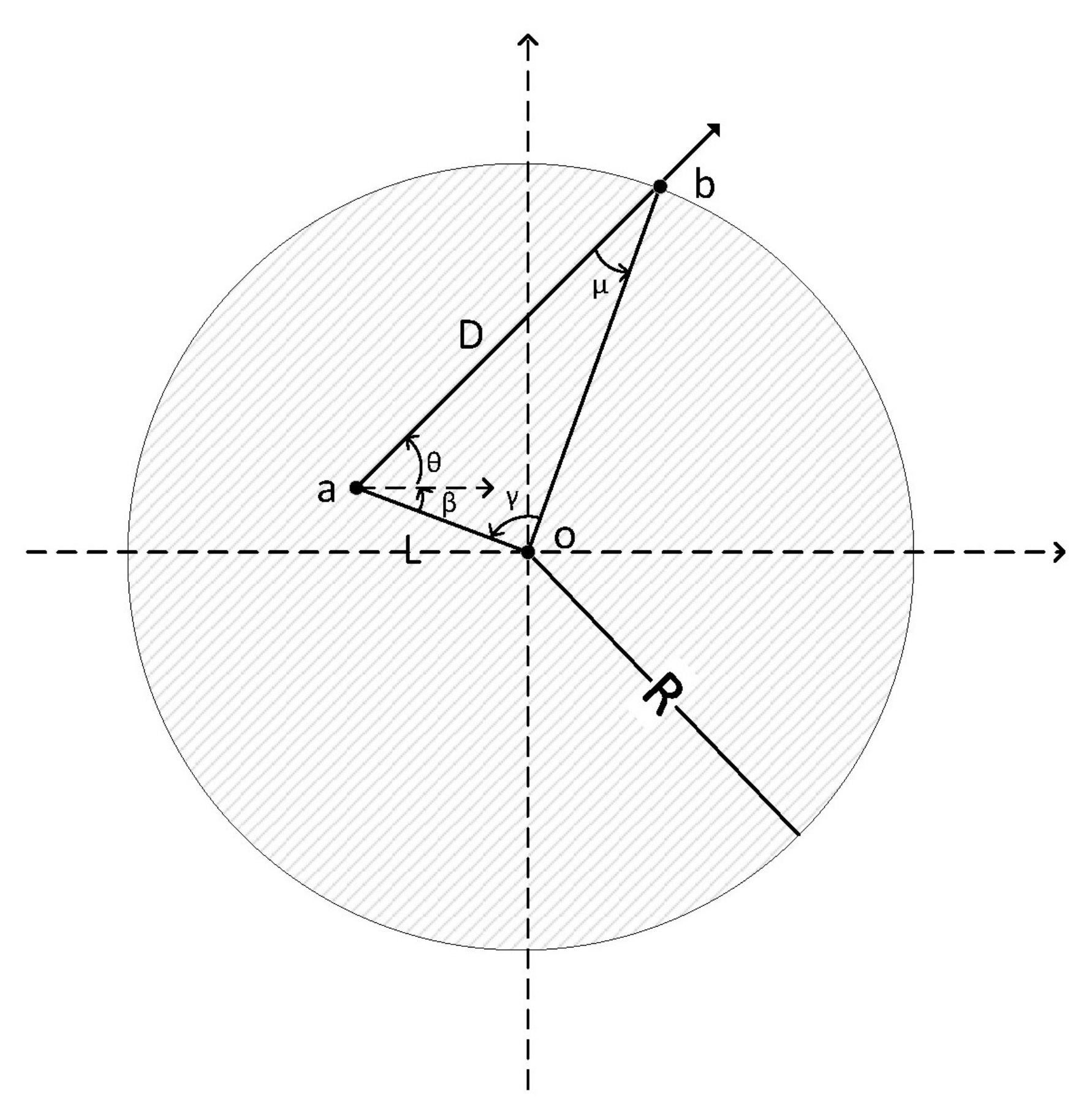
In the 5G network, the pico BSs have lots of computation tasks to solve. If the computation tasks exceed the computation capability of pico BSs and their computation units, such as MEC, pico BSs can offload the extra tasks to the stations with more powerful computation units, such as cloud computation units. However, the disadvantage of this solution is that the latency of the computation tasks transmission between pico BSs and cloud units cannot conform to the requirements.

Around the pico BSs, many UEs are equipping with computation units, including vehicles and mobile phones. These computation units are available to provide computation capability in a part of time. If the pico BSs aggregates the UEs into a cluster and split the computation task to every member in the cluster, the capability of the cluster is comparable to the capability of the cloud center unit. Meanwhile, short-distance between UEs and pico BSs can significantly reduce the computation task transmission latency compared to the cloud center unit.

UEs have two offloading states: busy and idle. UE in busy state means UEs are processing the computation tasks offloading, while idle state means UEs have no computation tasks. Because the computation capability of the UEs is weak, we assume that UE will use all available computation capability to solve the computation tasks. Therefore, accepting new tasks is not a practical option for busy UEs before they complete the ongoing computation tasks offloading. Only idle UEs that do not have computation tasks can accept new offloading. However, because the capability of UEs is different, the maximum number of tasks is unlimited, which means UEs can accept multiple tasks from different pico BSs simultaneously. In this situation, the computation capacity is allocated according to the task load. Then, the computation time $t_u^c$ is

$$\begin{array}{c}\hfill t_u^c=\sum _m\frac{S_{m,u}}{C_u}{G}_m,\end{array}$$

(4)

where $S_{m,u}\in (0,1)$ represents the proportion of the computation task that the pico BS m allocates to the UE u, $C_u$ is the computation capability of the UE u, and $G_m$ is the computation task load of pico BS m. The computation task load G is different for pico BSs.

Because the computation tasks from different pico BSs are different, multi-connectivity is not feasible for this. According to the Shannon–Hartley theorem, the transmission time of the computation task from pico BS m to UE u can be calculated as

$$\begin{array}{cc}\hfill t_{m,u}^s& =\frac{S_{m,u}{G}_m}{R_{m,u}^s}\hfill \\ & =\frac{S_{m,u}{G}_m}{B_{m,u}^{s}lo{g}_2(1+\frac{P_{m,u}{H}_{m,u}}{{\sum }_{j,j\ne m}{P}_{j,u}{H}_{j,u}+N_0})}\hfill \\ & =\frac{S_{m,u}{G}_m}{B_{m,u}^s{k}_{m,u}},\hfill \end{array}$$

(5)

where we replace $lo{g}_2(1+\frac{P_{m,u}{H}_{m,u}}{{\sum }_{j,j\ne m}{P}_{j,u}{H}_{j,u}+N_0})$ by $k_{m,u}$ for the simplification. Then, the time consumed by the computation task is the summary of transmission time and calculation time as $t_{m,u}=t_u^c+t_{m,u}^s$.

3.3. Moving Model

3.3.1. Vehicles

As shown in Figure 1, the system is based on the urban model. The vehicles run on the road, while the pedestrians move in the whole area. On the road, vehicles have two directions, forward or backward. They cannot change the direction, e.g., make a u-turn, while they are in the middle of the road. When they arrive at the crossing, three options can be chosen, go straight, turn left, and turn right. The probability of going straight, turn left, and turn right are 50%, 25%, and 25%, respectively. The velocity of the vehicles is changing all the time. We adopt the Gauss-Markov model as the principle of the velocity calculation [37]. Assume that the velocity of vehicles is constant within a time slot; then, we can get the relationship between the velocity at time t and the velocity at time $t+1$ as

$$\begin{array}{c}\hfill V_{t+1}^v=\alpha V_t^v+(1-\alpha )V^v+\sqrt{1-{\alpha }^2}{w}_t,\end{array}$$

(6)

where $\alpha \in \left[0,1\right]$ is the control parameter representing the randomness of the velocity, which is about the correlation between the velocities at different times, $w_t$ is the Gaussian random with zero mean and ${\sigma }^2$ variance, and $V^v$ keeping constant is the mean velocity of all vehicles. When $\alpha =1$, then, $V_{t+1}^v=V_t^v$, which means the velocity is constant. On the contrary, when $\alpha =0$, then, $V_{t+1}^v=V^v+w_t$, which means the velocity is random and independent of the previous movement. Based on Equation (6), we can get the velocity after time $k(k\in N^0)$ as

$$\begin{array}{c}\hfill V_{t+k}^v={\alpha }^k{V}_t^v+(1-{\alpha }^k)V^v+\sqrt{1-{\alpha }^2}\sum _{i=0}^{k-1}{\alpha }^{k-i-1}{w}_{t+i}.\end{array}$$

(7)

Based on the promise that the velocity in a time slot $\Delta t$ is constant, the total distance from time slot t to time slot $t+k$ is

$$\begin{array}{cc}\hfill D& =\sum _{j=0}^k\Delta t{V}_{t+j}^v\hfill \\ & =\Delta t\left\{V_t^v+\sum _{j=1}^k\left[{\alpha }^j{V}_t^v+(1-{\alpha }^j)V^v+\sqrt{1-{\alpha }^2}\sum _{i=0}^{j-1}{\alpha }^{j-i-1}{w}_{t+i}\right]\right\}\hfill \\ & =\Delta t\left[\frac{1-{\alpha }^k}{1-\alpha }{V}_t^v+(k-\frac{1-{\alpha }^k}{1-\alpha })V^v+\sqrt{1-{\alpha }^2}\sum _{j=1}^k\sum _{i=0}^{j-1}{\alpha }^{j-i-1}{w}_{t+i}\right].\hfill \end{array}$$

(8)

For $w_t$ as a Gaussian random, according to the character of the Gaussian distribution, the summary of the independent Gaussian random still follows the Gaussian distribution. Therefore, ${\sum }_{j=0}^k{\sum }_{i=0}^{j-1}{\alpha }^{j-i-1}{w}_{t+i}$ in (9) is also a Gaussian random. The mean is zero and variance is $\frac{{\sigma }^2(1-{\alpha }^2)}{{(1-\alpha )}^2}{(k-\frac{1-{\alpha }^{k-1}}{1-\alpha })}^2$. The first and the second part of Equation (9) is constant. Finally, total distance D is a Gaussian random with mean $\Delta t\left[\frac{1-{\alpha }^k}{1-\alpha }{V}_t^v+(k-\frac{1-{\alpha }^k}{1-\alpha })V^v\right]$ and variance ${\Delta }^{2}t\frac{{\sigma }^2(1-{\alpha }^2)}{{(1-\alpha )}^2}{(k-\frac{1-{\alpha }^{k-1}}{1-\alpha })}^2$.

When vehicles are at the crossing, they can go straight, turn left, or turn right. The probability of not going out the area of the pico BSs under these three choices can be set as $P_u^s=P(D\le D_u^s),P_u^l=P(D\le D_u^l),P_u^r=P(D\le D_u^r)$, respectively. The probability of staying within the area of pico BSs in a certain time can be calculated as

$$\begin{array}{c}\hfill P_u^v=0.5P_u^s+0.25P_u^l+0.25P_u^r.\end{array}$$

(9)

3.3.2. Pedestrians

Pedestrians move on the whole area. The Random Way Point (RWP) model is a widely used moving model to demonstrate the trail of pedestrians [38] and is also adopted by our article. In this model, a pedestrian chooses a destination randomly in the whole area, then chooses a random velocity $V^p$ and random staying time $t^s$ in the feasible region $[V^{min},V^{max}]$ and $[t^{min},t^{max}]$, respectively. Firstly, the pedestrian moves to the destination with velocity $V^p$. After arriving at the destination, the pedestrian will stay at the destination for time $t^s$. Then, the pedestrian chooses a new destination and repeats the procedures mentioned above. Pico BSs transmit the computation tasks to the pedestrians only if the pedestrians are within the area of pico BSs. After moving out of the area of pico BSs, the transmission will terminate.

If pedestrians pass the area of pico BSs, the trail of pedestrians can be divided into two situations. The first one is that the destination is within the area of pico BSs. The second one is that the destination is without the area of pico BS, but a part of the trail is within the area of pico BSs. In the first situation, pedestrians will stay in the area of pico BSs before going to the new destination. The stay time of pedestrians $t^s$ can be considered larger than the needed computation task transmission time. In the second situation, after getting the information about location and direction, as well as the velocity of pedestrians, the distance $D_u$ that pedestrian goes out the area of the pico BSs can be calculated.

As illustrated in Figure 2, o point is the pico BS with coordinates ($x_1$,$y_1$), a point is the pedestrian with coordinates ($x_2$,$y_2$), b point is the location that pedestrian move out the area of pico BS, and $\theta$ is the direction of movement. $D_u$ can be calculated using these parameters as

$$\begin{array}{cc}\hfill D_u& =\frac{Rsin\gamma }{sin(\theta +\beta )}\hfill \\ & =\sqrt{R^2-{\left[sin\theta (x_2-x_1)-cos\theta (y_2-y_1)\right]}^2}-cos\theta (x_2-x_1)-sin\theta (y_2-y_1).\hfill \end{array}$$

(10)

According to Equation (9), the probability that pedestrian can complete the transmission of computation task is $P_u^p=P(D_u\le t^t{V}_u^p)$, where $t^t$ is the computation task transmission time.

3.3.3. Transmission Time Limit

According to Equation (9), the distribution of the distance that users go through is Gaussian. The mean and variance of the distribution are about the moving time slot k, the origin velocity $V_t$ and the mean velocity for all users V. For independent UE, the maximum available transmission time is equal to the moving time determined by the distance mentioned above. The moving time in Equation (9) is discrete, different from the transmission time which is continuous. To unify these two variables, we transfer the variance and mean in Equation (9) as follows,

$$\begin{array}{cc}\hfill variance& ={\Delta }^{2}t\frac{{\sigma }^2(1-{\alpha }^2)}{{(1-\alpha )}^2}{(k-\frac{1-{\alpha }^{k-1}}{1-\alpha })}^2\hfill \\ & =\frac{{\sigma }^2(1+\alpha )}{(1-\alpha )}{(k\Delta t-\Delta t\frac{1-{\alpha }^{k-1}}{1-\alpha })}^2\hfill \\ & =\frac{{\sigma }^2(1+\alpha )}{(1-\alpha )}{(t-\Delta t\frac{1-{\alpha }^{k-1}}{1-\alpha })}^2\hfill \end{array}$$

(11)

$$\begin{array}{cc}\hfill mean& =\Delta t\left[\frac{1-{\alpha }^k}{1-\alpha }{V}_t^v+(k-\frac{1-{\alpha }^k}{1-\alpha })V\right]\hfill \\ & =\Delta t\frac{1-{\alpha }^k}{1-\alpha }(V_t^v-V)+\Delta tkV\hfill \\ & =\Delta t\frac{1-{\alpha }^k}{1-\alpha }(V_t^v-V)+tV.\hfill \end{array}$$

(12)

Let the time slot $\Delta t$ tend to be infinitesimal, and the time in (9) can be seen as continuous. Then, the variance and mean are $\frac{(1+\alpha )}{(1-\alpha )}{(\sigma t)}^2$ and $tV$, separately.

The success of transmission cannot be guaranteed because of the random movement. We consider that pico BSs have the error tolerance $\delta$ for the transmission. Transmission is deemed successful if the ratio of the unfinished transmission is less than $\delta$.

3.4. Incentive Model

For UEs involved in the computation task offloading, the awards are necessary to offset energy consumption and the loss of throughput. Communication resources are good rewards for UEs because every UE needs bandwidth to communicate. Therefore, we adopt bandwidth as the reward to stimulate UE to involve computation offloading.

At the beginning of the offloading, pico BSs propose offers to UEs, and then UEs decide whether to accept or reject according to the characteristics of the devices. If the offer is smaller than the price of UE, UE will reject. Then, BSs improve the offer and repeat the above processes again and again until they reach agreement. The offloading will happen many times. After several rounds, the system reaches steady state, and BSs know the relationship between minimum price and the characteristics of every UE. We assume the system is in the steady state, and the offer from BSs is the minimum price in the paper.

The characteristics include conditions and requirements of UE. The condition of the UEs is different. For example, the computation capability and the energy of vehicles are much larger than that of mobile phones. Vehicles have more tolerance for resource consumption than pedestrians. We define the tolerance factor $l_u=\frac{C_u}{C}$ to depict this character, where C represents the computation capability baseline. Additionally, the bandwidth requirement is different among UEs. The requirement is much more urgent for the UEs with real-time traffic, e.g., online video or surfing the internet, than for those with no real-time traffic, e.g., downloading. The requirement factor $d_u$ is defined to depict this character. Overall, the larger $l_u$ is, the more willing to join the offloading UEs have. The larger $d_u$ is, the less willing to join the offloading UEs have.

For the pico BSs, the rewards for computation task offloading are one of their biggest concerns. If the reward for UE is bigger than the revenue from task offloaded, pico BSs are not eager to do the offloading. The task load $S_{m,u}{G}_m$, tolerance factor $l_u$, and requirement factor $d_u$ determine the rewards for every UE. We define the minimum incentive for UE u to join the task offloading as $\frac{S_{m,u}{G}_m}{l_u{d}_u}$. If the rewards that pico BSs provide are larger than the minimum incentive, UE will join the task offloading. After accepting the proposal, the bandwidth that UE is allocated is $1+\frac{S_{m,u}{G}_m}{l_u{d}_u}$ times as much as before. Then, the rate of UE u for communication $R_u^{*}$ is

$$\begin{array}{cc}\hfill R_u^{*}& =(1+\sum _m\frac{S_{m,u}{G}_m}{l_u{d}_u})B_u^{d}lo{g}_2\left[1+\frac{{\sum }_m{F}_{m,u}{P}_{m,u}{H}_{m,u}}{{\sum }_m(1-F_{m,u})P_{m,u}{H}_{m,u}+N_0}\right]\hfill \\ & =(1+\sum _m\frac{S_{m,u}{G}_m}{l_u{d}_u})B_u^{d}lo{g}_2\left[\frac{{\sum }_m{P}_{m,u}{H}_{m,u}+N_0}{{\sum }_m(1-F_{m,u})P_{m,u}{H}_{m,u}+N_0}\right].\hfill \end{array}$$

(13)

3.5. Problem Formulation

MCDC contains throughput improvement and computation offloading expenses. To balance the revenue from computation task offloading and the variation of communication rate, we define the utility function as the function of offloading size and transmission rate

$$\begin{array}{cc}\underset{{\mathcal{B}}^d,{\mathcal{B}}^s,\mathcal{S},\mathcal{F}}{max}\hfill & \Theta =\sum _u\sum _m{S}_{m,u}{G}_m+\beta \sum _u{R}_u^{*}\hfill \\ & \mathrm{s}.\mathrm{t}.\hfill \\ & (c_{14.1})B_u^d,B_{m,u}^s\in N^0\hfill & \forall m\in \mathcal{M},u\in \mathcal{U}\hfill \\ & (c_{14.2})S_{m,u}\in (0,1)\hfill & \forall m\in \mathcal{M},u\in \mathcal{U}\hfill \\ & (c_{14.3})F_{m,u}\in \left\{0,1\right\}\hfill & \forall m\in \mathcal{M},u\in \mathcal{U}\hfill \\ & (c_{14.4})\sum _u{S}_{m,u}\le 1\hfill & \forall m\in \mathcal{M}\hfill \\ & (c_{14.5})\sum _u\left[(1+\sum _m\frac{S_{m,u}{G}_m}{l_u{d}_u})B_u^d{F}_{m,u}+B_{m,u}^s\right]\le W\hfill & \forall m\in \mathcal{M}\hfill \\ & (c_{14.6})(1+\sum _m\frac{S_{m,u}{G}_m}{l_u{d}_u})B_u^d+\sum _m{B}_{m,u}^s\le W\hfill & \forall u\in \mathcal{U}\hfill \\ & (c_{14.7})t_{m,u}^c+t_{m,u}^s\le t\hfill & \forall u\in \mathcal{U}\hfill \\ & (c_{14.8})(1-p_u)S_{m,u}\le \delta \hfill & \forall m\in \mathcal{M}\hfill \\ & (c_{14.9})B_u^d\le W_{max}\hfill & \forall u\in \mathcal{U},\hfill \end{array}$$

(14)

where $\beta$ is the adjustment factor for offloading size and transmission rate. Constraint ($c_{14.1}$) represents the feasible area of the communication bandwidth and offloading bandwidth, respectively. Constraint ($c_{14.2}$) represents the feasible area of the proportion of the offloading task. Constraint ($c_{14.3}$) represents the feasible area of the connection between UEs and pico BSs in communication. Constraint ($c_{14.4}$) prohibits the offloading task to all UEs exceeding the total task size. In Constraint ($c_{14.5}$), the first part $(1+{\sum }_m\frac{S_{m,u}{G}_m}{l_u{d}_u})B_u^d{F}_{m,u}$ and the second part $B_{m,u}^s$ on the right side of equation is the bandwidth that pico BS m allocated to UE u for communication and computation task offloading, respectively. Constraint ($c_{14.5}$) ensures that the total available bandwidth of pico BS m is less than the system bandwidth W. The correspondent of constraint ($c_{14.5}$) is constraint ($c_{14.6}$). Different from the traditional resource allocation, constraint ($c_{14.6}$) is added in the optimization to ensure that the bandwidth allocated to UE u from different pico BSs is not overlapping. Because of the multi-connectivity, a UE can associate with multiple pico BSs. Though with the guarantee of constraining ($c_{14.5}$) the allocated bandwidth from pico BS is not larger than total bandwidth W, the bandwidth allocated to UE u from different pico BSs could be the same then overlapping, which is against to Equation (4). Constraint ($c_{14.7}$) represents the limitation of time for task offloading, where t is the maximum allowable time. Constraint ($c_{14.8}$) represents the error tolerance of pico BSs for the computation task offloading. Constraint ($c_{14.9}$) promises the fairness of the bandwidth allocation, where $W_{max}$ is the maximum bandwidth for a single UE.

4. Co-Scheduling of Communication and Computation Optimization

The problem (14) involves both integer (F) and continuous ($B^d,B^s,S$) optimization variables with non-linear functions, which is a typical Mixed Integer Non-linear Programming (MINLP) problem. Generally, MINLP is hard to solve as they combine the difficulty of optimizing over integer variables with the handling of non-linear functions. We split the integer and continuous variables and then figure out the optimal result by a two-step optimization.

4.1. Branch and Bound Method for Integer Variables

For integer variables F, with every feasible individual $B^{d*},B^{s*},S^{*}$, the utility function (14) can be reconstructed as

$$\begin{array}{cc}\hfill \underset{\begin{array}{c}\mathcal{F}\end{array}}{max}\sum _u& \left[(1+\sum _m\frac{S_{m,u}{G}_m}{l_u{d}_u})B_u^{d}lo{g}_2(\frac{{\sum }_m{P}_{m,u}{H}_{m,u}+N_0}{{\sum }_m(1-F_{m,u})P_{m,u}{H}_{m,u}+N_0})\right]\hfill \\ & \mathrm{s}.\mathrm{t}.\hfill \\ & (c_{14.3})F_{m,u}\in \left\{0,1\right\}\hfill & \forall m\in \mathcal{M},u\in \mathcal{U}\hfill \\ & (c_{14.5})\sum _u\left[(1+\sum _m\frac{S_{m,u}^{*}{G}_m}{l_u{d}_u})B_u^{d*}{F}_{m,u}+B_{m,u}^{s*}\right]\le W\hfill & \forall m\in \mathcal{M}.\hfill \end{array}$$

(15)

Integer variables (F) are contained in a very complex non-linear function. The only way to find the optimal parameter is the branch-and-bound method. To maximize the throughput, UEs with high received signals are prior to bandwidth. Based on this premise, the branch follows the sequence of the received signal from largest to smallest. On the other hand, ($c_{14.9}$) restricts the maximum bandwidth for a single UE, which means the value of UEs associated to every BSs is $\lceil W/W_{max}\rceil$, where $\lceil ·\rceil$ means rounding up an integer. The feasible area of UE is top $\lceil W/W_{max}\rceil$ UE of every BSs according to the sequence.

4.2. Continuous Variables with Barrier Function

Obviously, the utility function (14) and constraints $(c_{14.4})$, $(c_{14.5})$, as well as $(c_{14.6})$, $(c_{14.7})$, are convex about variables ($B^d,B^s,S$). To verify Constraint $(c_{14.8})$’s convexity is very complex. For convenience, $(c_{14.8})$ is developed to full form as

$$\begin{array}{c}\hfill \left[1-\frac{\sqrt{1-\alpha }}{\sigma t\sqrt{2\pi (1+\alpha )}}{\int }_{-\infty }^{D_u}{e}^{-\frac{{(x-tV)}^2(1-\alpha )}{2(1+\alpha ){(\sigma t)}^2}}dx\right]·S_{m,u}\le \delta .\end{array}$$

(16)

Let $z=\frac{(1-\alpha )}{2(1+\alpha ){(\sigma )}^2}$, substituting $y=\sqrt{{(\frac{x}{t}-V)}^{2}z}$ into (16), and we obtain

$$\begin{array}{ccc}& & \left[1-\sqrt{\frac{z}{\pi t^2}}{\int }_{-\infty }^{D_u}{e}^{-y^2}d(\sqrt{\frac{1}{z}}ty+tV)\right]·S_{m,u}\le \delta \hfill \\ \hfill then& & \left[1-\sqrt{\frac{1}{\pi }}{\int }_{-\infty }^{\sqrt{z}(\frac{D_u}{t}-V)}{e}^{-y^2}dy\right]·S_{m,u}\le \delta ,\hfill \end{array}$$

(17)

where t is the moving time for UE, which can be seen as the maximum transmission time $t_{m,u}^s$ for the computation task, substituting $t_{m,u}^s=\frac{S_{m,u}{G}_m}{B_{m,u}^s{k}_{m,u}}$ into (17), and then

$$\begin{array}{c}\hfill f(B^s,S)=\left[1-\sqrt{\frac{1}{\pi }}{\int }_{-\infty }^{\sqrt{z}(\frac{B_{m,u}^s{k}_{m,u}{D}_u}{S_{m,u}{G}_m}-V)}{e}^{-y^2}dy\right]·S_{m,u}-\delta \le 0.\end{array}$$

(18)

To verify the convexity of (18), take the derivative of (18) for $B^s$ as

$$\begin{array}{ccc}\hfill f{(B^s)}^{\prime }& & =-\sqrt{\frac{z}{\pi }}{S}_{m,u}·e^{-z{(\frac{B_{m,u}^s{k}_{m,u}{D}_u}{S_{m,u}{G}_m}-V)}^2}\frac{k_{m,u}{D}_u}{S_{m,u}{G}_m}\hfill \\ & & =-\sqrt{\frac{z}{\pi }}\frac{k_{m,u}{D}_u}{G_m}·e^{-z{(\frac{B_{m,u}^s{k}_{m,u}{D}_u}{S_{m,u}{G}_m}-V)}^2},\hfill \end{array}$$

(19)

and the second derivative for $B^s$ of (18) as

$$\begin{array}{c}\hfill f{(B^s)}^{″}=\sqrt{\frac{4z^3}{\pi }}\frac{k_{m,u}^2{D}_u^2}{S_{m,u}{G}_m^2}(\frac{B_{m,u}^s{k}_{m,u}{D}_u}{S_{m,u}{G}_m}-V)e^{-z{(\frac{B_{m,u}^s{k}_{m,u}{D}_u}{S_{m,u}{G}_m}-V)}^2}.\end{array}$$

(20)

It is easy to find the part $(\frac{B_{m,u}^s{k}_{m,u}{D}_u}{S_{m,u}{G}_m}-V)$ decides the positive or negative of (20). Noticing that $t_{m,u}^s=\frac{S_{m,u}{G}_m}{B_{m,u}^s{k}_{m,u}}$, substitute $t_{m,u}^s$ into the above part as $(\frac{D_u-tV}{t})$. Constraint $(c_{14.8})$ ensures that the error data size for the computation task offloading is smaller than the tolerance $\sigma$ that is very small, which means error probability $p_u$ also needs to be small enough, e.g., several percent. To ensure this point, according to the character of Gaussian Distribution, distance $D_u$ has to be much larger than the mean $t{V}^v$, which means $(\frac{D_u-tV}{t})>0$.

Next, take the derivative of (18) for S as

$$\begin{array}{c}\hfill f{(S)}^{\prime }=\left[1-\sqrt{\frac{1}{\pi }}{\int }_{-\infty }^{\sqrt{z}(\frac{B_{m,u}^s{k}_{m,u}{D}_u}{S_{m,u}{G}_m}-V)}{e}^{-y^2}dy\right]+\sqrt{\frac{z}{\pi }}{e}^{-z{(\frac{B_{m,u}^s{k}_{m,u}{D}_u}{S_{m,u}{G}_m}-V)}^2}\frac{B_{m,u}^s{k}_{m,u}{D}_u}{S_{m,u}{G}_m},\end{array}$$

(21)

and the second derivative for S of (18) is

$$\begin{array}{ccc}\hfill f{(S)}^{″}=& & \sqrt{\frac{z}{\pi }}{e}^{-z{(\frac{B_{m,u}^s{k}_{m,u}{D}_u}{S_{m,u}{G}_m}-V)}^2}\frac{B_{m,u}^s{k}_{m,u}{D}_u}{S_{m,u}^2{G}_m}\hfill \\ & & +\sqrt{\frac{z}{\pi }}{e}^{-z{(\frac{B_{m,u}^s{k}_{m,u}{D}_u}{S_{m,u}{G}_m}-V)}^2}\frac{B_{m,u}^s{k}_{m,u}{D}_u}{S_{m,u}^2{G}_m}2z(\frac{B_{m,u}^s{k}_{m,u}{D}_u}{S_{m,u}{G}_m}-V)\frac{B_{m,u}^s{k}_{m,u}{D}_u}{S_{m,u}{G}_m}\hfill \\ & & -\sqrt{\frac{z}{\pi }}{e}^{-z{(\frac{B_{m,u}^s{k}_{m,u}{D}_u}{S_{m,u}{G}_m}-V)}^2}\frac{B_{m,u}^s{k}_{m,u}{D}_u}{S_{m,u}^2{G}_m}\hfill \\ \hfill =& & 2\sqrt{\frac{z^3}{\pi }}{e}^{-z{(\frac{B_{m,u}^s{k}_{m,u}{D}_u}{S_{m,u}{G}_m}-V)}^2}\frac{B_{m,u}^{s2}{k}_{m,u}^2{D}_u^2}{S_{m,u}^3{G}_m^2}(\frac{B_{m,u}^s{k}_{m,u}{D}_u}{S_{m,u}{G}_m}-V),\hfill \end{array}$$

(22)

and we have proven $(\frac{B_{m,u}^s{k}_{m,u}{D}_u}{S_{m,u}{G}_m}-V)>0$; therefore, (22) is positive, and then (18) is convex about S. To solve the programming, we conduct the barrier function by logarithmic function as

$$\begin{array}{ccc}\hfill \Gamma =& & -\gamma \sum _m\sum _u{S}_{m,u}{G}_m-\gamma \beta \sum _u{R}_u-\sum _{u}log(B_u^d)-\sum _m\sum _{u}log(B_{m,u}^s)-\sum _m\sum _{u}log(S_{m,u})\hfill \\ & & -\sum _{u}log(1-\sum _u{S}_{m,u})-\sum _{u}log\left\{W-\sum _u\left[(1+\sum _m\frac{S_{m,u}{G}_m}{l_u{d}_u})B_u^d{F}_{m,u}+B_{m,u}^s\right]\right\}\hfill \\ & & -\sum _{u}log\left[W-(1+\sum _m\frac{S_{m,u}{G}_m}{l_u{d}_u})B_u^d-\sum _m{B}_{m,u}^s\right]-\sum _m\sum _{u}log(t-t_{m,u}^c-t_{m,u}^s)\hfill \\ & & -\sum _m\sum _{u}log\left[\delta -(1-p_u)S_{m,u}\right],\hfill \end{array}$$

(23)

where $\gamma$ is penalty factor. Both utility function (14) and constraints $(c_{14.4})$, $(c_{14.5})$, $(c_{14.6})$, $(c_{14.7})$, as well as $(c_{14.8})$, have been proven to be convex. Hence, barrier function $\Gamma (B^d,B^s,S)$ is also convex. We propose the total algorithm about parameters $(F,B^d,B^s,S)$ in Algorithm 1.

Algorithm 1: Co-scheduling of Communication and Computation.

Initially$\tau =10$, $\omega =0.01$, $\beta =0.5$,$\epsilon =0.01;$,$\zeta =0.01$,$k=0.01;$     $B^d$ satisfying $(c_{14.1})$, $(c_{14.5})$, $(c_{14.6})$, $(c_{14.9})$,$B^s=0,S^{}=0$, $y=(B^d,B^s,S^{})$;

1: Repeat

2:    Branch and bound $F_k$ following policy with parameters $y_k$

3:    $\gamma :=1,x=y_k;$

4:    While $2m·u/\gamma \ge \omega$

5:       Do

6:          $\Delta x=-{\nabla }^2{\Gamma }^{-1}\nabla \Gamma$;            ${\lambda }^2=\nabla \Gamma {\nabla }^2{\Gamma }^{-1}\nabla \Gamma$;

7:          If ${\lambda }^2/2\le \epsilon$

8:            Break

9:          End

10:          $\mu :=1;$

11:          If $\Gamma (x+\mu \Delta x)-\Gamma (x)-\omega \mu \nabla \Gamma \Delta x\le 0$

12:             $\mu :=\beta \mu$;

13:          End

14:          $x:=x+\mu \Delta x$;

15:       End

16:       $\gamma :=\tau \gamma$;

17:    End

18:    If $\Theta (F_k,y_k)-\Theta (F_{k-1},y_{k-1})<\zeta$

19:       Break

20:    End

21:    $k:=k+1,y_k:=x;$

22: End

5. Performance Evaluations and Simulation Results

In this section, we evaluate the performance of the multi-connectivity enhanced offloading scheme with system-level simulations using MATLAB R2017a. The offloading ratio is illustrated in the following paragraph compared with cloud offloading. Throughput under the influence of computation offloading is also demonstrated in this part.

5.1. Simulation Setting

According to the system model, we consider a system that comprises regular streets, pico BSs, pedestrians, and vehicles. Streets are North-South direction and East-West direction. The distance between two adjoining parallel streets is 200 m. In the area of 400 m times 400 m, there are 12 pico BSs with 120 pico UEs and 40 vehicles. Every four pico BSs form a cluster. The pico UEs are evenly distributed in the cluster area, which is around 100 m in diameter. Vehicles run on the street with different locations, directions, and velocities. The width of the street is neglected when calculating distances regarding the location of vehicles. We apply cyclic boundary conditions to the system when calculating the SINR. The pathlossmodel is based on 3GPP TR 36.814 [39] and TR 36.872 [40]. To avoid the influence of the system scale, which can be extended by just replication and translational movement of the original system, the results about throughput and offloading size will be divided by the value of pico BSs, which means the results mentioned above are mean values about one pico BS. The system configuration is summarized in

Table 2. System configuration.

Parameter	Value
Number of pico BSs	12
Number of pedestrians	120
Number of Vehicles	40
Power of pico BSs per 10 MHz	30 dBm
Power of Gaussian noise per 10 MHz	−95 dBm
Bandwidth of pico BSs	2–20 MHz
Computation task size G	1–20 MB
Time limit t	0.5–10 s
Computation capability multiplier $mt$	1–20
Mean velocity of pedestrians $V^p$	1 m/s
Mean velocity of vehicles $V^v$	10 m/s
Control parameter $\alpha$	0.5
Computation baseline C	1
Requirement factor $d_u$	0.5–1
Adjustment parameter $\beta$	0.02
Variance $\sigma$	$\frac{1}{\sqrt{6}}{V}^v$

. The main parameters are based on the 3GPP standards [39,40].

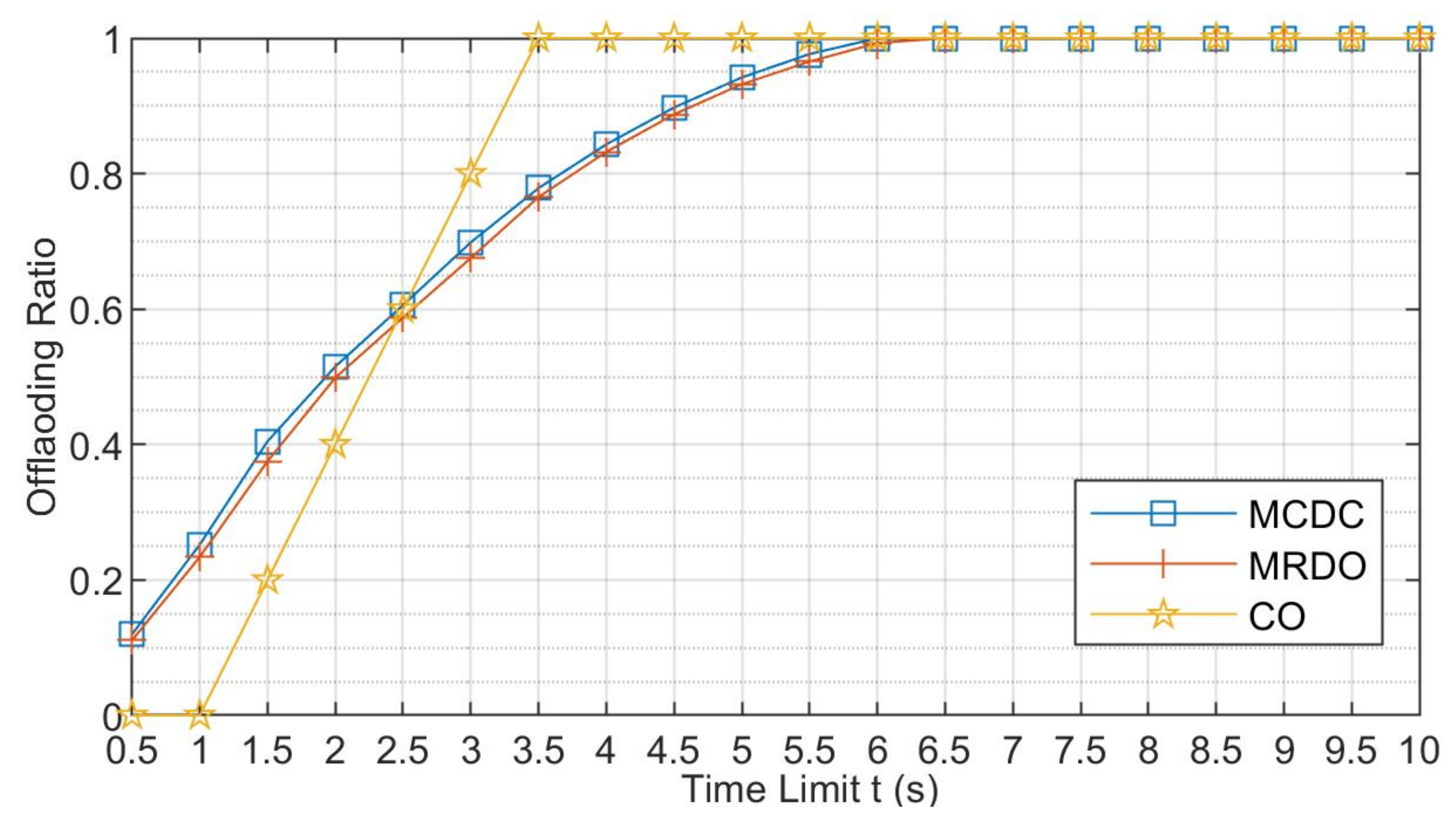
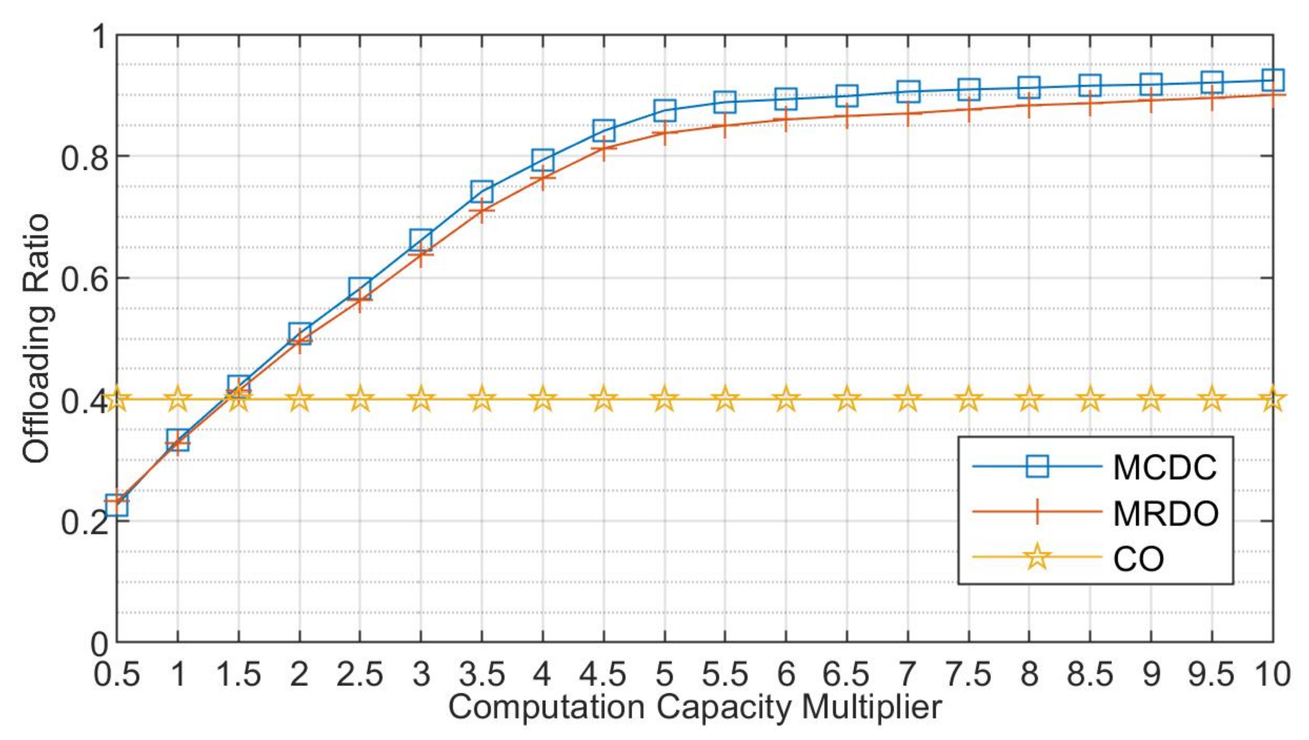
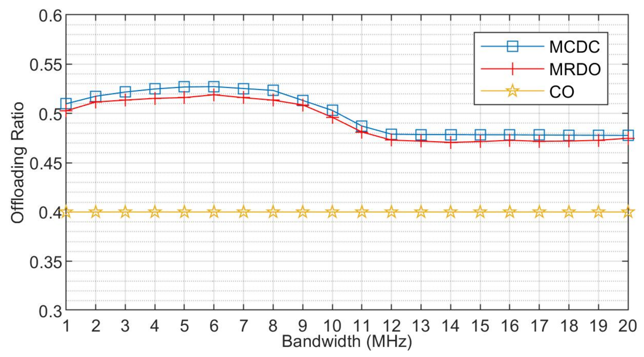
5.2. Simulation Results and Discussions

In the first place, we evaluate the computation offloading ratios with different strategies under various conditions. In the figures, MRDO means Max-RSRP Distributed Offloading, where UEs will choose the BS with Max-RSRP to access, and CO means Cloud Offloading. Unlike the unstable wireless channel, the link between BSs and the cloud is wired channels, such as optical fiber. The transmission speed of optical fiber is constant, the computation capacity of the cloud is also constant. Generally, the cloud is far away from pico BSs and UEs. The delay brought by the long-distance is non-negligible. We assume the inherent delay of optical fiber is 1 s. The computation task that cloud can be solved in 1 s, including transmission time and computing time, is 28.8 MB. To make the simulation as real as possible, the computation capacity of UEs is random. The actual capacity of pedestrians and vehicles are $0.1·mt·(1\pm 20\%)$ MB/s and $0.4·mt·(1\pm 20\%)$ MB/s, respectively, where $mt$ is the computation capability multipliers.

Figure 3 shows the offloading ratio of different strategies under various time limit t. For offloading to the cloud, the total delay includes a 1-s inherent delay. If the maximum tolerance for the time is less than 1 s, the cloud cannot complete the offloading task. As Figure 3 shows, with the time limit t ascend, the cloud can solve 28.8 MB computation task every second, which is 40% of the total 72 MB task. After 2.5 s, the cloud will accomplish the whole task. For the distributed methods, the computation capacity of UEs is only about 0.2 MB/s, which is 1/144 of the cloud. The computation capacity of vehicles is about 0.8 MB/s, which is 1/36 of the cloud. Despite this, UEs are close to pico BSs. UEs could receive the task without waiting for the signal transmitting. When the cloud begins to receive and calculate the task at t is 1 s, UEs have solved about 23% task. Although the cloud is greatly more powerful than UEs, it is dragged by the long distance. The advantage of the cloud emerges only the t is bigger than 2.5 s. In the area that t is less than 2.5 s, the offloading ratio of the distributed method is larger than that of the cloud method, which means the distributed method is a better way for the time-sensitive task.

Figure 4a depicts the offloading ratio using three different strategies under various loads. On the account that the capability of the cloud is constant, the offloading size will not change when the computation task load fluctuates. Therefore, the offloading ratio is a truncated inverse proportional function where the ratio is 100% in the area of load less than 2.4 MB. On the contrary, the offloading size of distributed mode ascends with the load, although the offloading ratio descends with the load, which can be obtained from Figure 4b. The offloading size will increase with the load because the utility function benefits from the increasing offloading size. While load grows to a point, UEs cannot adopt more computation tasks due to that the offloading of computation tasks occupies the bandwidth of communication. We can obtain this conclusion from Figure 4b. When the load is 10 MB, the offloading size will not rise. On the other hand, the offloading size cannot keep pace with the load increase, which leads to the decrease of offloading size. What has to be pointed out is that, when the load is less than 4 MB, offloading to the cloud is better than distributed offloading. Because the capacity of the cloud is constant, bandwidth does not influence offloading, which is different from distributed offloading. However, if decreasing the time limit, the cloud offloading ratio will be lower than distributed offloading.

The computation capacity is another critical factor to influence the offloading ratio. We can imply, from Figure 5, that distributed offloading ratio will exceed the cloud offloading ratio with computation capability increasing. The direct influential factor of offloading size is the time limit t that contains offloading time and computation time. Offloading bandwidth decides the offloading time, while computation capacity decides the computation time. According to (4) and ($c_{14.7}$), increasing the computation capacity will offload more computation tasks because the change of computation capacity does not directly disturb the throughput. At the same time, the offloading time restricts the increase of offloading size. The growth of offloading size will slow down with the computation capacity increasing. If the computation time is much less than offloading time, the offloading time will play a pivotal role. For example, let $t=2,t^c=0.1,t^s=1.9$. Doubling computation capability, offloading size only increases 2.56%. In this situation, the offloading size can be taken as constant, as shown in Figure 5.

Additionally, the offloading bandwidth competes with communication bandwidth that is nearly linearly related to the throughput. Allocation of bandwidth for offloading or communication depends on the utility function (14). If the computation capacity of UE is constant, the growth of offloading size will slow down with the offloading bandwidth increasing as Figure 6, which is different from the situation of transmission bandwidth. When bandwidth is small, the transmission of offloading tasks consumes much more time than computing. A little more offloading bandwidth greatly enlarges offloading size, while communication cannot get so much benefit from the same bandwidth. However, the profit from bandwidth decreases with bandwidth larger. Offloading gains the upper hand at about 6MHz and then descends. When the offloading ratio gets to a balancing point, the offloading ratio levels off because the decrease of offloading bandwidth impair unitality function.

From Figure 3, Figure 4, Figure 5 and Figure 6, we find that the offloading ratio of MCDC is larger than MRDO. With multi-connectivity, the interference can be translated into a useful signal. UEs can get higher transmission rates from the same bandwidth, which increases the offloading size. However, the gap between the two strategies is tiny because the bandwidth has little effect on the offloading size, which has been mentioned above. In Figure 6, the fluctuation of offloading ratio because of bandwidth is only 0.05, which can explain why the gap of multi-connectivity and Max-RSRP is less than 0.04.

On the contrary, the influence of multi-connectivity on throughput is much more than that on offloading size. In the second place, the throughput of different strategies under various conditions are illustrated in Figure 7, Figure 8, Figure 9 and Figure 10, where Multi-Connectivity Communication Only (MCCO) and Max-RSRP Communication Only (MRCO) strategies are without computation offloading. In the figures, Available Ratio means the throughput of other strategies divided by MCCO. According to figures, throughput can get 7.5~15.1% gain using multi-connectivity compared to the Max-RSRP, at most. If we choose the time limit, bandwidth, load, and computation capability as 2 s, 10 MHz, 6 MB, and 2, respectively, the offloading size of distributed and cloud methods are approximately equal. The loss of throughput from offloading using multi-connectivity is 13%. The loss of throughput from offloading using Max-RSRP is 21%. The improvement of multi-connectivity is 10.2%.

The computation of advanced algorithms, such as multi-connectivity, is much more complex than simple methods, such as Max-RSRP. If the computation workload of Max-RSRP is set as the capacity of BSs, offloading size will be the extra expense to realize the advanced algorithm. However, the computation offloading will decrease the throughput. This conflict underlines the importance of co-scheduling of communication and computation. By co-scheduling, the throughput will gain 11.9% compared to Max-RSRP. In Figure 7, we can see that, when the load is less than 6 MB, the throughput of MCDC is bigger than MRCO. Likewise, in Figure 8, when the computation multiplier is larger than 6.5, the performance of MCDC is better than MRCO. When the computation size of MCDC is the same as CO, the throughput will gain 5.8%.

The relationship between throughput and load is depicted in Figure 7. It is easy to understand that the offloading occupying a part of system bandwidth let throughput descend with load increasing. After the load is heavy enough, the load would not affect the throughput and offloading size anymore, which agrees with Figure 4 and Figure 7. Figure 8 shows the throughput under different computation capability multiples, where throughput initially descends and then ascends. Referring to Figure 5, when the computation capability multiplier is less than 5, throughput is decreasing, while the offloading size is increasing. When computation capability multiplier exceeds 5, throughput increases, while offloading size maintains constant. The offloading grabs a part of the bandwidth as computation capability is small. Then, communication recaptures bandwidth after offloading size is steady.

Figure 9 illustrates the relationship between throughput and time limit. According to (4) and (6), and ($c_{14.7}$), the offloading ratio is a nearly linear increase with the time limit, which means the time limit has little influence on offloading bandwidth. The bandwidth for communication keeps constants leading to constant throughput with the different time limits. On the contrary, it can be learned from Figure 10 that bandwidth is the primary factor influencing throughput. Because it is not involved in the offloading, the throughput of MCCO linearly relates to bandwidth. As the upper bound, the gap between MCCO and other strategies is the loss caused by offloading. When bandwidth is small, the gap is most conspicuous because the bandwidth is used for offloading to get more utility than communication, which has been discussed before. As bandwidth gets larger and larger, offloading bandwidth stops growing as the benefit from more offloading bandwidth is small than transmission bandwidth. The ratio of offloading bandwidth in total bandwidth keeps decreasing with total bandwidth increasing. Then, along comes that gap, little by little.

6. Conclusions

In the article, we propose a multi-connectivity enhanced co-scheduling scheme of communication resource allocation and distributed computation offloading. We choose to offload time-sensitive computation tasks to the UEs surrounding BSs to avoid the significant delay of cloud offloading. The scheme splits the computation task and distributes the pieces to nearby UEs, including vehicles and pedestrians added, to overcome the limit of computation capability of UEs. UEs are compensated and stimulated to join the offloading based on the communication incentive mechanism, where involved UEs will be allocated more bandwidth on throughput according to rewards factors decided by offloading size and UE characters, such as tolerance factor and requirement factor. The probability that UEs move out the area of BSs is calculated by analyzing the movement of vehicles and pedestrians based on two moving models. Offloading failure rate, which is a conclusive condition to decide the offloading size, is defined according to the above probability. Multi-connectivity is used to improve throughput and reduce the loss caused by offloading. The computation offloading enables BSs to achieve the more powerful performance, while bringing more workload than ever to the wireless communication. By the co-scheduling of the communication and computation scheme, the impairment brought by offloading workload is diminished. Moreover, the scheme helps that the benefit of offloading exceeds the damage of offloading. The system throughput is improved by the proposed scheme. The system-level simulation shows that the proposed scheme will improve 11.9% throughput compared to Max-RSRP and gain 5.8% throughput compared to cloud offloading.

References

1. Cisco. Cisco Visual Networking Index: Forecast and Trends. Available online: https://www.cisco.com/c/en/us/solutions/collateral/service-provider/visual-networking-index-vni/white-paper-c11-741490.html (accessed on 19 December 2018).
2. Feriani, A.; Hossain, E. Single and Multi-Agent Deep Reinforcement Learning for AI-Enabled Wireless Networks: A Tutorial. IEEE Commun. Surv. Tutor. 2021, 23, 1226–1252. [Google Scholar] [CrossRef]
3. Letaief, K.B.; Chen, W.; Shi, Y.; Zhang, J.; Zhang, Y.J.A. The Roadmap to 6G: AI Empowered Wireless Networks. IEEE Commun. Mag. 2019, 57, 84–90. [Google Scholar] [CrossRef] [Green Version]
4. Zhang, J.; Xu, X.; Zhang, K.; Han, S.; Tao, X.; Zhang, P. Learning Based Flexible Cross-layer Optimization for Ultra-reliable and Low Latency Applications in IoT Scenarios. IEEE Internet Things J. 2021. [Google Scholar] [CrossRef]
5. Zheng, J.; Cai, Y.; Wu, Y.; Shen, X. Dynamic Computation Offloading for Mobile Cloud Computing: A Stochastic Game-Theoretic Approach. IEEE Trans. Mob. Comput. 2019, 18, 771–786. [Google Scholar] [CrossRef]
6. Jalali, F.; Hinton, K.; Ayre, R.; Alpcan, T.; Tucker, R.S. Fog Computing May Help to Save Energy in Cloud Computing. IEEE J. Sel. Areas Commun. 2016, 34, 1728–1739. [Google Scholar] [CrossRef]
7. Zhang, K.; Mao, Y.; Leng, S.; He, Y.; Zhang, Y. Mobile-Edge Computing for Vehicular Networks: A Promising Network Paradigm with Predictive Off-Loading. IEEE Veh. Technol. Mag. 2017, 12, 36–44. [Google Scholar] [CrossRef]
8. Huang, X.; Yu, R.; Kang, J.; Zhang, Y. Distributed Reputation Management for Secure and Efficient Vehicular Edge Computing and Networks. IEEE Access 2017, 5, 25408–25420. [Google Scholar] [CrossRef]
9. Pillai, P.S.; Rao, S. Resource Allocation in Cloud Computing Using the Uncertainty Principle of Game Theory. IEEE Syst. J. 2016, 10, 637–648. [Google Scholar] [CrossRef]
10. You, C.; Huang, K.; Chae, H. Energy Efficient Mobile Cloud Computing Powered by Wireless Energy Transfer. IEEE J. Sel. Areas Commun. 2016, 34, 1757–1771. [Google Scholar] [CrossRef] [Green Version]
11. Chiu, T.; Pang, A.; Chung, W.; Zhang, J. Latency-Driven Fog Cooperation Approach in Fog Radio Access Networks. IEEE Trans. Serv. Comput. 2019, 12, 698–711. [Google Scholar] [CrossRef]
12. Dong, Y.; Guo, S.; Liu, J.; Yang, Y. Energy-Efficient Fair Cooperation Fog Computing in Mobile Edge Networks for Smart City. IEEE Internet Things J. 2019, 6, 7543–7554. [Google Scholar] [CrossRef]
13. Zhao, J.; Li, Q.; Gong, Y.; Zhang, K. Computation Offloading and Resource Allocation For Cloud Assisted Mobile Edge Computing in Vehicular Networks. IEEE Trans. Veh. Technol. 2019, 68, 7944–7956. [Google Scholar] [CrossRef]
14. Dai, Y.; Xu, D.; Maharjan, S.; Zhang, Y. Joint Load Balancing and Offloading in Vehicular Edge Computing and Networks. IEEE Internet Things J. 2019, 6, 4377–4387. [Google Scholar] [CrossRef]
15. Lin, C.; Han, G.; Qi, X.; Guizani, M.; Shu, L. A Distributed Mobile Fog Computing Scheme for Mobile Delay-Sensitive Applications in SDN-Enabled Vehicular Networks. IEEE Trans. Veh. Technol. 2020, 69, 5481–5493. [Google Scholar] [CrossRef]
16. Zeng, D.; Pan, S.; Chen, Z.; Gu, L. An MDP-Based Wireless Energy Harvesting Decision Strategy for Mobile Device in Edge Computing. IEEE Netw. 2019, 33, 109–115. [Google Scholar] [CrossRef]
17. Luo, S.; Chen, X.; Zhou, Z.; Chen, X.; Wu, W. Incentive-Aware Micro Computing Cluster Formation for Cooperative Fog Computing. IEEE Trans. Wirel. Commun. 2020, 19, 2643–2657. [Google Scholar] [CrossRef]
18. Han, S.; Xu, X.; Fang, S.; Sun, Y.; Cao, Y.; Tao, X.; Zhang, P. Energy Efficient Secure Computation Offloading in NOMA-Based mMTC Networks for IoT. IEEE Internet Things J. 2019, 6, 5674–5690. [Google Scholar] [CrossRef] [Green Version]
19. Gao, X.; Huang, X.; Bian, S.; Shao, Z.; Yang, Y. PORA: Predictive Offloading and Resource Allocation in Dynamic Fog Computing Systems. IEEE Internet Things J. 2020, 7, 72–87. [Google Scholar] [CrossRef]
20. Ge, X.; Sun, Y.; Gharavi, H.; Thompson, J. Joint Optimization of Computation and Communication Power in Multi-User Massive MIMO Systems. IEEE Trans. Wirel. Commun. 2018, 17, 4051–4063. [Google Scholar] [CrossRef]
21. Wang, Y.; Wang, K.; Huang, H.; Miyazaki, T.; Guo, S. Traffic and Computation Co-Offloading With Reinforcement Learning in Fog Computing for Industrial Applications. IEEE Trans. Ind. Inform. 2019, 15, 976–986. [Google Scholar] [CrossRef]
22. Hu, X.; Zhuang, X.; Feng, G.; Lv, H.; Wang, H.; Lin, J. Joint Optimization of Traffic and Computation Offloading in UAV-Assisted Wireless Networks. In Proceedings of the 2018 IEEE 15th International Conference on Mobile Ad Hoc and Sensor Systems (MASS), Chengdu, China, 9–12 October 2018; pp. 475–480. [Google Scholar] [CrossRef]
23. Feng, J.; Pei, Q.; Yu, F.R.; Chu, X.; Shang, B. Computation Offloading and Resource Allocation for Wireless Powered Mobile Edge Computing with Latency Constraint. IEEE Wirel. Commun. Lett. 2019, 8, 1320–1323. [Google Scholar] [CrossRef]
24. Yousefi, S.; Altman, E.; El-Azouzi, R.; Fathy, M. Analytical Model for Connectivity in Vehicular Ad Hoc Networks. IEEE Trans. Veh. Technol. 2008, 57, 3341–3356. [Google Scholar] [CrossRef]
25. Tang, X.; Xu, X.; Haenggi, M. Meta Distribution of the SIR in Moving Networks. IEEE Trans. Commun. 2020, 68, 3614–3626. [Google Scholar] [CrossRef]
26. Ma, W.; Fang, Y.; Lin, P. Mobility Management Strategy Based on User Mobility Patterns in Wireless Networks. IEEE Trans. Veh. Technol. 2007, 56, 322–330. [Google Scholar] [CrossRef]
27. Khabazian, M.; Ali, M.K.M. A Performance Modeling of Connectivity in VehicularAd Hoc Networks. IEEE Trans. Veh. Technol. 2008, 57, 2440–2450. [Google Scholar] [CrossRef]
28. Chandrashekar, S.; Maeder, A.; Sartori, C.; Höhne, T.; Vejlgaard, B.; Chandramouli, D. 5G multi-RAT multi-connectivity architecture. In Proceedings of the 2016 IEEE International Conference on Communications Workshops (ICC), Kuala Lumpur, Malaysia, 23–27 May 2016; pp. 180–186. [Google Scholar] [CrossRef]
29. Ravanshid, A.; Rost, P.; Michalopoulos, D.S.; Phan, V.V.; Bakker, H.; Aziz, D.; Tayade, S.; Schotten, H.D.; Wong, S.; Holland, O. Multi-connectivity functional architectures in 5G. In Proceedings of the 2016 IEEE International Conference on Communications Workshops (ICC), Kuala Lumpur, Malaysia, 23–27 May 2016; pp. 187–192. [Google Scholar] [CrossRef] [Green Version]
30. Du, L.; Zheng, N.; Zhou, H.; Chen, J.; Yu, T.; Liu, X.; Liu, Y.; Zhao, Z.; Qian, X.; Chi, J.; et al. C/U Split Multi-Connectivity in the Next Generation New Radio System. In Proceedings of the 2017 IEEE 85th Vehicular Technology Conference (VTC Spring), Sydney, Australia, 4–7 June 2017; pp. 1–5. [Google Scholar] [CrossRef]
31. Zhang, K.; Xu, X.; Zhang, J.; Zhang, B.; Tao, X.; Zhang, Y. Dynamic Multiconnectivity Based Joint Scheduling of eMBB and uRLLC in 5G Networks. IEEE Syst. J. 2021, 15, 1333–1343. [Google Scholar] [CrossRef]
32. Zhang, B.; Xu, X.; Zhang, K.; Zhang, J.; Guan, H.; Zhang, Y.; Zhang, Y.; Zheng, N.; Teng, Y. Goodput-Aware Traffic Splitting Scheme with Non-ideal Backhaul for 5G-LTE Multi-Connectivity. In Proceedings of the 2019 IEEE Wireless Communications and Networking Conference (WCNC), Marrakech, Morocco, 15–19 April 2019; pp. 1–6. [Google Scholar] [CrossRef]
33. Wolf, A.; Schulz, P.; Dörpinghaus, M.; Filho, J.C.S.S.; Fettweis, G. How Reliable and Capable is Multi-Connectivity? IEEE Trans. Commun. 2019, 67, 1506–1520. [Google Scholar] [CrossRef] [Green Version]
34. Suer, M.; Thein, C.; Tchouankem, H.; Wolf, L. Multi-Connectivity as an Enabler for Reliable Low Latency Communications—An Overview. IEEE Commun. Surv. Tutor. 2020, 22, 156–169. [Google Scholar] [CrossRef]
35. Petrov, V.; Solomitckii, D.; Samuylov, A.; Lema, M.A.; Gapeyenko, M.; Moltchanov, D.; Andreev, S.; Naumov, V.; Samouylov, K.; Dohler, M.; et al. Dynamic Multi-Connectivity Performance in Ultra-Dense Urban mmWave Deployments. IEEE J. Sel. Areas Commun. 2017, 35, 2038–2055. [Google Scholar] [CrossRef]
36. Liu, R.; Yu, G.; Li, G.Y. User Association for Ultra-Dense mmWave Networks With Multi-Connectivity: A Multi-Label Classification Approach. IEEE Wirel. Commun. Lett. 2019, 8, 1579–1582. [Google Scholar] [CrossRef]
37. Musolesi, M.; Mascolo, C. Designing Mobility Models based on Social Network Theory. ACM SIGMOBILE Mob. Comput. Commun. Rev. 2007, 11, 59–70. [Google Scholar] [CrossRef]
38. Zhang, L.; Leng, S.; Cook, S.C. Effects of mobility on stability in vehicular ad hoc networks. In Proceedings of the 2010 IEEE 6th International Conference on Wireless and Mobile Computing, Networking and Communications, Chengdu, China, 23–25 September 2010; pp. 707–712. [Google Scholar] [CrossRef]
39. 3GPP. Evolved Universal Terrestrial Radio Access (E-UTRA); Further Advancements for E-UTRA Physical Layer Aspects. Tech. Rep 36.814, 3GPP. v9.0.0. 2010. Available online: https://portal.3gpp.org/desktopmodules/Specifications/SpecificationDetails.aspx?specificationId=2493 (accessed on 10 October 2021).
40. 3GPP. Small Cell Enhancements for E-UTRA and E-UTRAN—Physical Layer Aspects. Tech. Rep 36.872, 3GPP. v12.1.0. 2013. Available online: https://portal.3gpp.org/desktopmodules/Specifications/SpecificationDetails.aspx?specificationId=2573 (accessed on 10 October 2021).
Figure 1. System model. The urban area is split by the parallel and perpendicular road into several rectangular part. Macro BaseStations (BSs) and pico BSs are located on the parts, and pedestrians are distributed around BSs, while vehicles run on the road.
Electronics 10 02466 g001
Figure 2. Movement of pedestrian when in the area of BS. Point o is location of BS, and point a is location of pedestrian, while point b is the location pedestrian moves out of area of BS whose radius is R.
Electronics 10 02466 g002
Figure 3. Offloading ratios under different time limits. Offloading task per pico BS is 6 MB. Bandwidth of BSs is 10 MHz. Computation capability multiplier is 2, which means the computation capability of pedestrians and vehicles are 0.16~0.24 MB/s and 0.64~0.96 MB/s, respectively.
Electronics 10 02466 g003
Figure 4. Offloading sizes and offloading ratios under various loads. Time limit t is 2 s. Bandwidth of BSs is 10 MHz. Computation capability multiplier is 2.
Electronics 10 02466 g004
Figure 5. Offloading ratios under different computation capability multipliers. Time limit t is 2 s. Offloading task per pico BS is 6 MB. Bandwidth of BSs is 10 MHz.
Electronics 10 02466 g005
Figure 6. Offloading ratios under different bandwidth. Time limit t is 2 s. Offloading task per pico BS is 6 MB. Computation capability multiplier is 2.
Electronics 10 02466 g006
Figure 7. Throughput of different strategies under various load. Time limit is 2 s. Bandwidth is 10 MHz. Computation capability multiplier is 2.
Electronics 10 02466 g007
Figure 8. Throughput of different strategies under various computation capability multipliers. Time limit is 2 s. Offloading task per pico BS is 6 MB. Bandwidth is 10 MHz.
Electronics 10 02466 g008
Figure 9. Throughput of different strategies under various time limit. Offloading task per pico BS is 6 MB. Bandwidth is 10 MHz. Computation capability multiplier is 2.
Electronics 10 02466 g009
Figure 10. Throughput of different strategies under various time limit. Offloading task per pico BS is 6 MB. Bandwidth is 10 MHz. Computation capability multiplier is 2.
Electronics 10 02466 g010