Article

Design of Integrated Autonomous Driving Control System That Incorporates Chassis Controllers for Improving Path Tracking Performance and Vehicle Stability

1
Graduate School of Automotive Engineering, Kookmin University, Seoul 02707, Korea
2
Department of Automotive Engineering, Kookmin University, Seoul 02707, Korea
*
Author to whom correspondence should be addressed.
Electronics 2021, 10(2), 144; https://doi.org/10.3390/electronics10020144
Submission received: 23 November 2020 / Revised: 30 December 2020 / Accepted: 5 January 2021 / Published: 11 January 2021
(This article belongs to the Section Systems & Control Engineering)

Abstract

:
This paper describes an integrated autonomous driving (AD) control system for an autonomous vehicle with four independent in-wheel motors (IWMs). The system consists of two parts: the AD controller and the chassis controller. These elements are functionally integrated to improve vehicle stability and path tracking performance. The vehicle is assumed to employ an IWM independently at each wheel. The AD controller implements longitudinal/lateral path tracking using proportional-integral(PI) control and adaptive model predictive control. The chassis controller is composed of two lateral control units: the active front steering (AFS) control and the torque vectoring (TV) control. Jointly, they find the yaw moment to maintain vehicle stability using sliding mode control; AFS is prioritized over TV to enhance safety margin and energy saving. Then, the command yaw moment is optimally distributed to each wheel by solving a constrained least-squares problem. Validation was performed using simulation in a double lane change scenario. The simulation results show that the integrated AD control system of this paper significantly improves the path tracking capability and vehicle stability in comparison with other control systems.

1. Introduction

Recently, there have been many efforts to develop path tracking algorithms since they are essential in autonomous driving (AD) maneuvers such as lane following, lane change, and collision avoidance. There are methods based on kinematic vehicle models [1,2,3,4] including the pure pursuit method and the Stanley method. However, by not considering a vehicle’s dynamics, these methods may not properly resolve stability issues that can occur when the vehicle is undergoing severe lateral motions. Secondly, there are methods based on dynamic vehicle models that can overcome the stability problems of kinematic methods. Various control schemes such as model predictive control (MPC) and linear quadratic regulator (LQR); and H-infinity, fuzzy, and genetic algorithms have been adopted to achieve reliable path tracking capabilities [5,6,7,8,9,10,11,12,13,14,15,16,17,18,19].
Many of the recent studies have adopted the MPC method and its variants. MPC is similar to LQR in that both methods compute control values by solving optimization problems. However, MPC solves an optimization problem in smaller time windows at every sample, while LQR uses a single optimal solution computed off-line for the whole time horizon. MPC can handle nonlinear models and constraints while LQR cannot. After optimizing for a finite number of samples including the current step and several future steps, MPC takes only the current step’s solution for control action. By repeatedly doing this at every sample, MPC has the capability of predicting future events that other conventional controllers such as PID do not have.
Ji et al. [11] adopted MPC with multiple constraints for steering control to avoid crashes with the vehicle ahead. Yoshida et al. [12] considered constraints on the tire forces and applied MPC for lane change control. Nam et al. [13] considered characteristics of the electric power steering system and achieved steering control with a quick response by using MPC. Gao et al. [14] applied nonlinear model predictive control (NMPC) to steering and braking control to develop obstacle avoidance logic. Rafaila et al. [15] considered nonlinear tire models and implemented steering control by NMPC.
Similar to any other linear control design method, the performance of MPC can deteriorate when the driving conditions deviate significantly from the setpoint where the model was linearized—for example, when the vehicle speed changes greatly or when the yaw motion becomes large. NMPC can be a solution to this problem, since it allows nonlinearities in the model, in the cost function, and in the constraints. However, this versatility of NMPC can be unfavorable for control purposes, since the nonlinear optimization problem can be nonconvex, and its minimum may not be found soon enough [16].
Adaptive model predictive control (AMPC) is another variant of MPC that can update model parameters such as mass, cornering stiffness, and velocity. Lin et al. [17] adopted AMPC for path tracking with consideration of tire cornering stiffness and road friction. Ercan et al. [18] considered the dynamic properties of the steering system and applied AMPC for steering control. Petersson et al. [19] divided the vehicle model into two categories, a low-speed model and a high-speed model, and applied AMPC to the high-speed model to achieve steering control.
There have been research efforts to design integrated chassis control systems for AD path tracking, and many of these studies considered the integration of electronic stability control (ESC) and active front steering (AFS). Both ESC and AFS generate a yaw moment to enhance lateral vehicle stability, but they work in different ways. ESC generates a yaw motion by differential braking, while AFS generates a yaw motion by additional steering. Since both controllers generate a yaw motion, their integration requires careful investigation of both synergistic and conflicting effects when they are working together. Yim et al. [20] integrated ESC and AFS using a weighted pseudo-inverse-based control allocation method that produces an algebraic solution. Zhang et al. [21] integrated a direct yaw moment and AFS using a null-space-based control reallocation method. Cho W et al. [22] formulated an optimization problem with an objective integrating ESC and AFS and solved the problem using the Karush–Kuhn–Tucker method.
Since electric vehicles are becoming popular, a powertrain system equipped with four independent in-wheel motors (IWMs) is drawing attention from the automotive industry [23,24,25,26,27]. This system enables torque vectoring (TV), since any combination of the longitudinal forces at the four wheels is possible with each wheel independently delivering tractive, braking, or zero force. Unlike ESC, TV can generate a yaw motion without decelerating the vehicle. The fact that a motor’s output torque can be estimated with ease and accuracy is another advantage of IWM-equipped electric vehicles for TV control implementation [28].
In this paper, an integrated AD control system is proposed for an autonomous vehicle with four independent IWMs. The system consists of an AD controller and a chassis controller that are functionally integrated to achieve improved vehicle stability and path tracking performance. The AD controller implements longitudinal/lateral path tracking control using PI control and AMPC. The chassis controller is composed of two lateral control units: AFS control and TV control. Jointly, they find the yaw moment to maintain the vehicle stability using sliding mode control, where AFS is prioritized over TV to enhance the safety margin and save energy. Then, the command yaw moment is optimally distributed to each wheel by solving a constrained least-squares problem.
The contributions of this study can be summarized as follows. There have been many studies for improving vehicle stability in lateral chassis control and also many studies for improving the path tracking performance in AD, but there have been few studies that consider both at the same time. As AD technology advances, both objectives should be considered together since they both contribute significantly to the safety of the autonomous vehicle but often affect each other in conflicting ways. To address this problem, an integrated AD control system that consists of the AD controller and the chassis controller has been developed in this study. The proposed algorithm was tested on various scenarios, and the simulation results verified that the proposed algorithm could significantly improve both path tracking capability and vehicle stability compared with other control systems.
This paper is organized as follows: Section 2 introduces the vehicle models used to design the controllers. Section 3 discusses the AD controller; it describes how the desired acceleration was computed for longitudinal control and how AMPC was designed for path tracking. Section 4 describes how the chassis controller improves vehicle stability by integrating the control of AFS and TV. Section 5 presents the simulation results that validate the proposed control system, and Section 6 concludes the paper.

2. Vehicle Modeling

This chapter introduces the vehicle models that were used in this study. Two different models were used to design the integrated AD control system. Since AFS affects a vehicle’s yaw motion only by steering action, a 2 degree of freedom (DOF) vehicle model that accounts for the lateral vehicle motion in response to the front steering angle was used for AFS. Since TV achieves yaw motion by having different rotational torques at each of the four wheels, a 7-DOF vehicle model that accounts for the wheel spin dynamics at each wheel was used for TV.

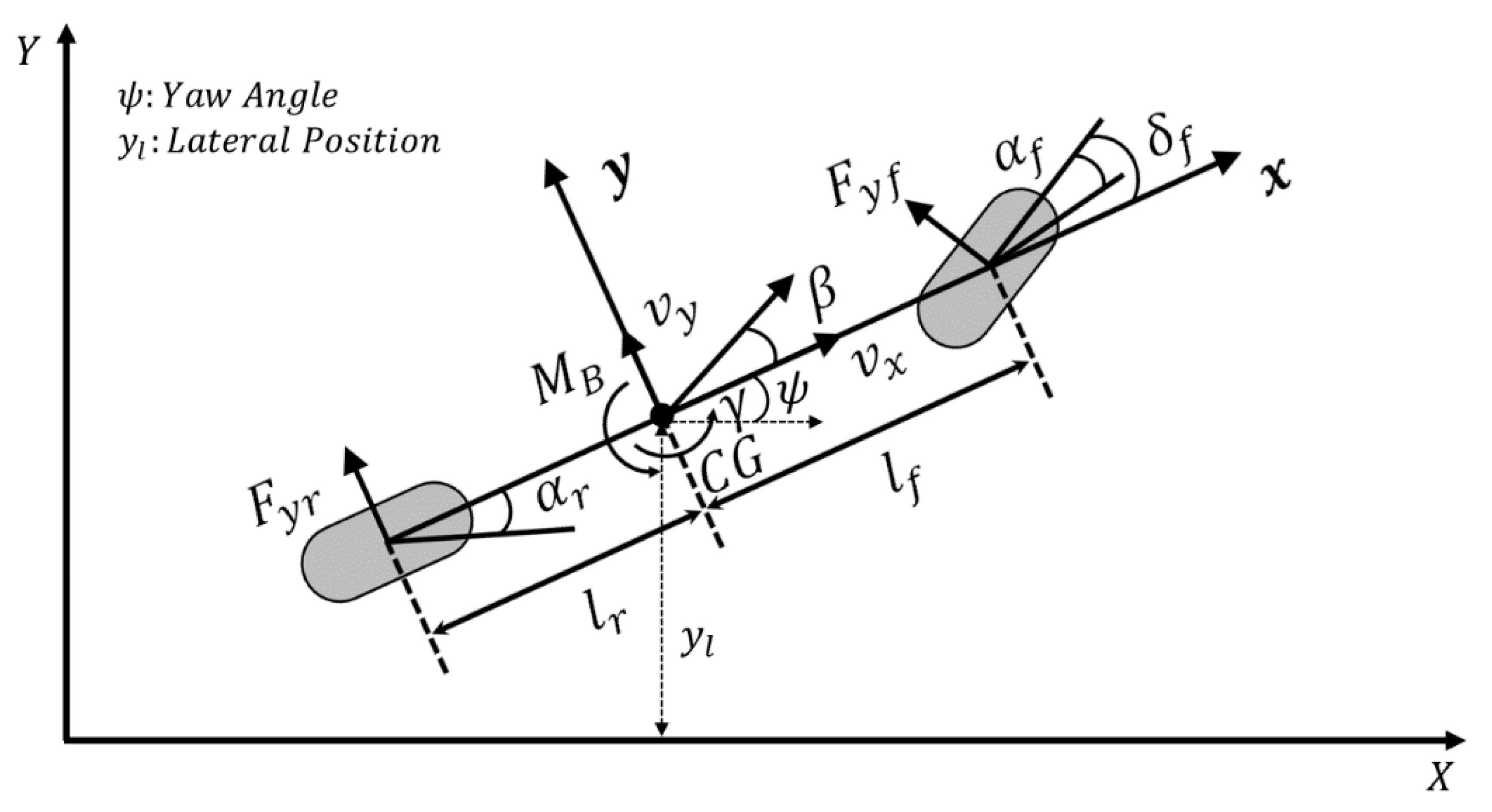
2.1. Vehicle Model for Path Tracking

Figure 1 shows the 2-DOF vehicle model, also known as a bicycle model, that accounts for the lateral translational motion and the yaw motion. Equation (1a,b) are the corresponding equations of motion [29].
m v x ( β ˙ + γ ) = F y f + F y r
I z γ ˙ = l f F y f l r F y r + M B
In this paper, the subscripts (   ) f and (   ) r are used to denote the front wheel and the rear wheel, respectively. In Equation (1a,b), m is the vehicle mass, l f is the distance from CG to the front axle, l r is the distance from CG to the rear axle, I z is the moment of inertia of the vehicle about the z-axis, v x is the longitudinal vehicle speed, γ is the yaw rate, β is the side-slip angle of the vehicle, F y (   ) is the lateral force at each wheel, and M B is the yaw moment that acts on the vehicle body.
Equation (2) shows the lateral tire model used in the above vehicle model.
F y f = 2 C f α f ,     F y r = 2 C r α r
In Equation (2), C (   ) is the cornering stiffness and α (   ) is the wheel slip angle. Each wheel slip angle can be computed from the variables in Equation (3a,b) as follows:
α f = δ f β l f γ v x
α r = β + l r γ v x .
To implement path tracking control, the vehicle’s location with respect to global coordinates is required. Equation (4a–c) show the kinematic equations to this end where ψ and y l represent the yaw angle and the lateral vehicle position, respectively, relative to global coordinates. Since ψ and β are small when they are properly controlled, Equation (4b) was linearized as Equation (4c).
ψ ˙ = γ
y ˙ l = v x ( s i n ψ + t a n β c o s ψ )
y ˙ l = v x ( ψ + β )

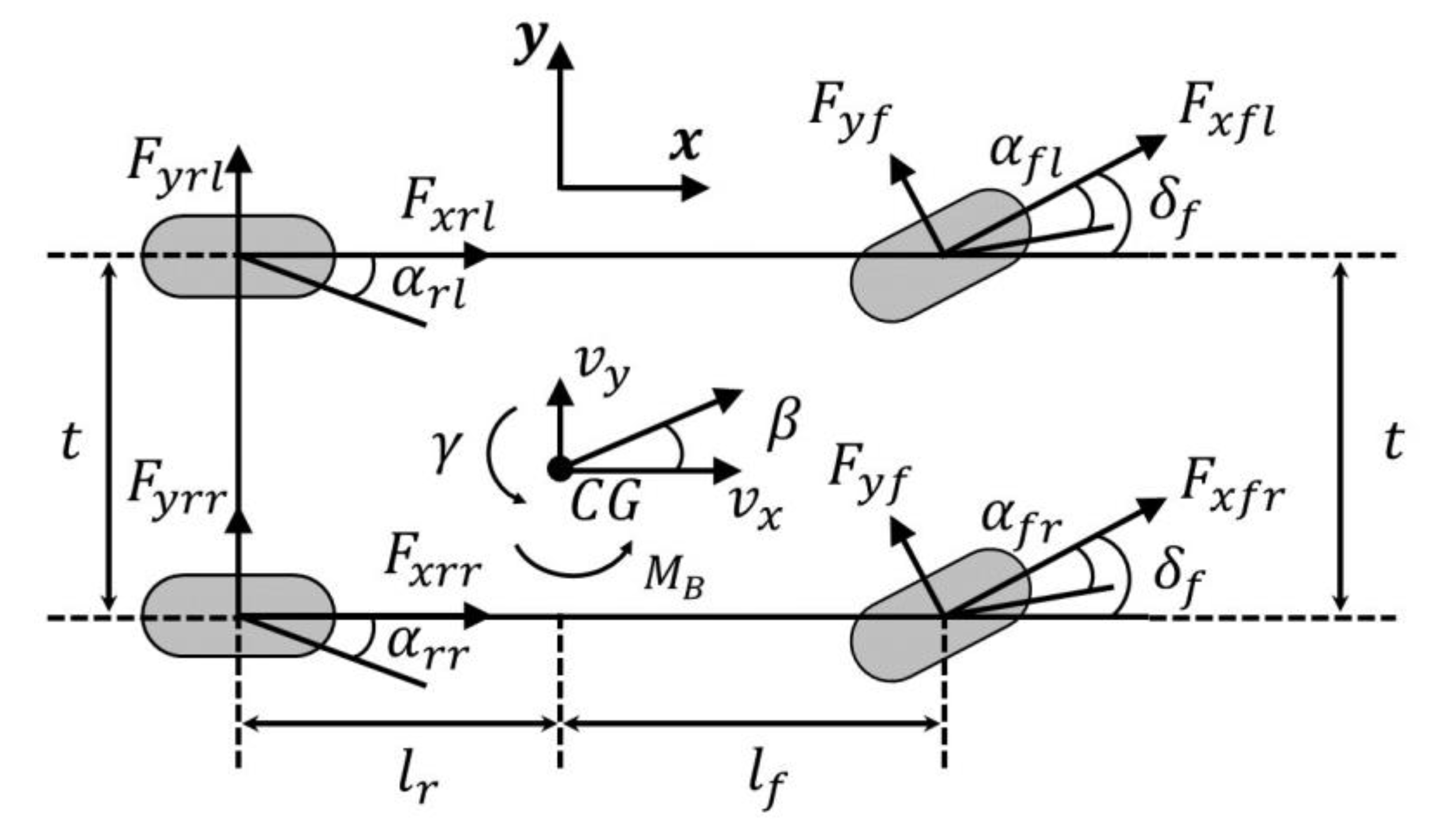
2.2. Vehicle Model for Torque Vectoring

Figure 2 shows the 7-DOF vehicle model used to develop the TV controller [30]. This model is composed of three equations to represent the vehicle body dynamics plus four equations to represent the wheel dynamics. The 2-DOF vehicle model in the previous section cannot be used here, since it does not contain the wheel dynamics that are necessary to implement the TV control logic. In contrast, the 7-DOF vehicle model is not appropriate for the AFS controller, since AFS does not need to consider wheel dynamics. It is common practice to use the lowest order vehicle model for controller design, since it will minimize the computational load when implementing the control logic on a real electronic control unit (ECU).
Equation (5a–c) describe vehicle body dynamics.
m x ¨ = ( F x f l + F x f r ) cos δ f + F x r l + F x r r ( F y f l + F y f r ) sin δ f + m γ y ˙
m y ¨ = F y r l + F y r r + ( F x f l + F x f r ) sin δ f + ( F y f l + F y f r ) cos δ f m γ y ˙
I z γ ˙ = l f ( F x f l + F x f r ) sin δ f + l f ( F y f l + F y f r ) cos δ f l r ( F y r l + F y r r ) + t 2 ( F x f r F x f l ) cos δ f + t 2 ( F x r r F x r l ) + t 2 ( F y f l F y f r ) sin δ f + M B
In Equation (5), the subscripts (   ) f l , (   ) f r , (   ) r l , and (   ) r r are used to indicate the location of the tire: front left, front right, rear left, and rear right, respectively. The parameters and variables used previously in Equations (1)–(4) have the same meanings in Equation (5). Additionally, t is the track width, x is the displacement in the local x-axis, y is the displacement in the local y-axis, F x (   ) is the longitudinal tire force, and F y (   ) is the lateral tire force.
The equations of Equation (6) show the rotational dynamics of the four tires.
J w ω ˙ i j = T w i j r e f f F x i j r e f f F x i j ,       i = f ,   r ,       j = r ,   l
In Equation (6), J w is the rotational moment of inertia of a tire, r e f f is the effective radius of a tire, and ω (   ) is the rotational velocity of each wheel. T w (   ) is the driving torque to each wheel, which is positive for traction and negative for braking.

3. AD Controller

Figure 3 shows the overall architecture of the integrated AD control system that was designed for this study. It consists of the AD controller and the chassis controller.
The AD controller performs the longitudinal/lateral path control of the vehicle. For longitudinal control, a proportional-integral(PI) controller was designed for acceleration control. For lateral control, the target path of the vehicle was planned at the current vehicle position, and steering control with AMPC was performed for path tracking. A time delay of 0.01 s was added to the model to account for the sampling interval of 100 Hz, which most chassis controllers adopt. The AMPC logic was made to work at an even slower 20 Hz sampling interval to allow for its heavy computational load, which is more than that of the PI controller. The details of the AD controller are presented in the following sections.

3.1. Longitudinal Controller

As seen in Figure 3, the AD controller consists of a longitudinal controller and a lateral controller. Since the main focus of this study lies in designing the lateral controller, a relatively simple PI control method was used to design the longitudinal controller. That controller performs acceleration control so that the autonomous vehicle can run at the desired speed v d e s .
To do this, the controller first computes the desired acceleration a d e s with Equation (7a).
a d e s = { a r e f i f   | a r e f | a u p p e r a u p p e r   s i g n ( a r e f )       o t h e r w i s e }
w h e r e a r e f = k a ( v d e s v x ) v x
The magnitude of the desired acceleration is limited by its upper bound a u p p e r to prevent excessive acceleration or deceleration. In Equation (7b), k a serves as a design parameter for computing the desired acceleration from the velocity error. A large k a results in a large desired acceleration value and vice versa. Careful tuning is necessary for k a , since it affects the performance of the TV logic that follows; a large k a strengthens speed tracking, but at the same time, it lessens the maintenance of vehicle stability. k a was set to 10 for this study. Once the desired acceleration is computed, acceleration control is performed by the PI controller. Since this PI controller has a straightforward and simple structure, its details are omitted in this paper.

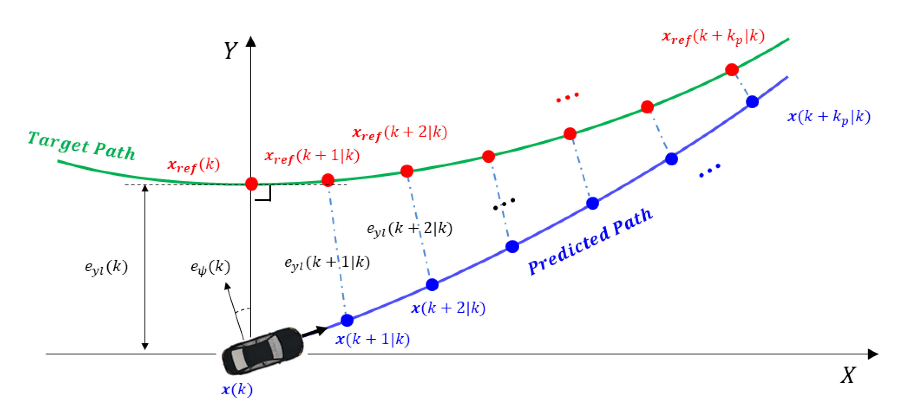
3.2. Lateral Controller

The lateral control function of the AD controller is implemented with AMPC. The motivation for adopting AMPC in this study can be explained by comparing it with the pure pursuit method, which is widely used in lateral control logic in autonomous vehicles. AMPC and pure pursuit are similar in that both methods compute the steering angle so that the vehicle follows the target path that lies ahead, but while Pure Pursuit sets a single waypoint in front as the target point to pass through, AMPC considers multiple waypoints within a certain time horizon. This improves lateral vehicle stability while achieving good path tracking performance. AMPC also allows considers control usage, while pure pursuit does not. Finally, only AMPC provides a lateral position error after a certain time horizon with steering control accounted for. This error data allows a good desired yaw moment to be computed to further improve the lateral vehicle stability and path tracking performance.
AMPC works by predicting the future behavior of a system by using two finite-time horizons: the prediction horizon and the control horizon. The prediction horizon is a multiple of the sampling period for which the state variables are predicted. The control horizon is the time interval in which the control variables are computed by solving an optimization problem. Until recently, MPC was hardly used in the field of vehicle control, since most vehicle controllers use in-vehicle sensors that can only detect what is currently happening, but MPC is beginning to draw attention since many of today’s vehicles are equipped with environmental sensors that can reveal what will shortly happen to the vehicle.
Choosing wider horizons in AMPC allows the controller to see farther into the future so it can be prepared for coming dangers. However, wider horizons can cause an ECU computational burden since the prediction is done by solving an optimization problem at every sample for the horizon interval. Given this, the prediction horizon is normally selected to be between 20 and 30, and the control horizon is selected to be 1/4 to 1/3 of the prediction horizon [31]. For this paper, the prediction horizon was set to 20 and the control horizon was set to 6.
The process of converting the original system equations into a form relevant for AMPC is described below. Equations (1)–(4) can be put into the compact form shown in Equation (8a–c) where x represents the state and u represents the control.
x ˙ = A x + B u
where     x = [ β γ ψ y l ] T ,     u = δ f
A = [ 2 ( C f + C r ) m v x 1 2 ( C f l f C r l r ) m v x 2 0 0 2 ( C f l f C r l r ) I z 2 ( C f l f 2 + C r l r 2 ) I z v x 0 0 0 1 0 0 v x 0 v x 0 ] ,    B = [ 2 C f m v x 2 l f C f I z 0 0 ]
To implement the optimization process required by AMPC, the above system can be transformed into a recursive form in discrete state space. First, A and B in Equation (8c) are converted into their discrete-time forms with T representing the sampling time:
A ¯ k = e A T
B ¯ k = k T ( k + 1 ) T e A [ ( k + 1 ) T τ ] B d τ .
Then, the state at k + k p , where k p denotes the prediction horizon, can be derived as below. In Equation (10c), k c denotes the control horizon.
x ( k + 1 | k ) = A ¯ k x ( k ) + B ¯ k u ( k )
x ( k + 2 | k ) = A ¯ k x ( k + 1 | k ) + B ¯ k u ( k + 1 ) = A ¯ k 2 x ( k ) + A ¯ k B ¯ k u ( k ) + B ¯ k u ( k + 1 )
x ( k + k p | k ) = A ¯ k k p x ( k ) + A ¯ k k p 1 B ¯ k u ( k ) + A ¯ k k p 2 B ¯ k u ( k + 1 ) + + A ¯ k k p k c B ¯ k u ( k + k c 1 ) .
Figure 4 illustrates how the target path is computed.
In Figure 4, x ( k + m | k ) is the state estimation at m samples after the current step, which is calculated by AMPC based upon the current state. Out of the four elements of the state vector in Equation (8b), the third element, the fourth element, the lateral position, and the yaw angle, respectively, represent the path of the vehicle. In the figure, x r e f ( k + m | k ) represents the target path of the vehicle m samples later.
Equation (11a–e) formulate the optimization problem for AMPC to find the front steering angle to track the vehicle’s desired path.
m i n   u ˜   m = 1 k p | | x r e f ( k + m | k ) x ( k + m | k ) | | Q 2 + m = 0 k c 1 | | u ( k + m | k ) | | R 2
s u b j e c t   t o         x ^ ( k + 1 ) = A ^ k   x ^ ( k ) + B ^ k u ^ ( k )
u m i n u ( k + m | k ) u m a x   ,         m = 0 , , k c 1
Δ u m i n Δ u ( k + m | k ) Δ u m a x   ,       m = 1 , , k c 1
where     Δ u ( k ) = u ( k ) u ( k 1 )            
For Equation (11b), A ^ k and B ^ k are defined in Equation (12a), and x ^ ( k + 1 ) and u ^ ( k ) are defined in Equation (12b).
A ^ k = [ A ¯ k A ¯ k 2 A ¯ k k p ]   ,     B ^ k = [ B ¯ k 0 0 A ¯ k B ¯ k B ¯ k 0 A ¯ k k p 1 B ¯ k A ¯ k k p 2 B ¯ k A ¯ k k p k c B ¯ k ]
x ^ ( k + 1 ) = [ x ˜ ( k + 1 | k ) x ˜ ( k + 2 | k ) x ˜ ( k + k p | k ) ]   ,     u ^ ( k ) = [ u ˜ ( k ) u ˜ ( k + 1 | k ) u ˜ ( k + k c 1 | k ) ]
Equation (11c) prevents the excessive use of the front steering angle, and Equation (11d) prevents an excessive change of the front steering angles between adjacent samples. Breuer et al. demonstrated that a driver can turn a steering wheel by 250 degrees with an angular rate of up to 1000 degrees per second [32]. However, when such a severe steering input is applied to an autonomous vehicle, its stability can be seriously endangered. In this design, the maximum front steering angle and its maximum change rate are limited to the values in Equation (13a,b) to retain vehicle stability. They roughly correspond to 90 [deg] of the steering wheel angle with 600 [deg/s] of the steering wheel angle rate.
u m i n = 0.0044 ,     u m a x = 0.0044
Δ u m i n = 0.029 ,     Δ u m i n = 0.029
In Equation (11a), Q and R are the weights for the state and the control, respectively. Equation (14) shows their values as used in this study. The first two diagonal elements in Q are zero because the corresponding state elements, the side-slip angle β , and the yaw rate γ are not directly related to the vehicle path.
Q = [ 0 0 0 0 0 0 0 0 0 0 1.5 0 0 0 0 10.3 ] ,     R = 96.5

4. Chassis Controller

As seen in Figure 3, the chassis controller of this study consists of two layers: the upper chassis controller and the lower chassis controller. The upper chassis controller computes the desired yaw moment from the yaw rate error and the lateral position error. The lower chassis controller realizes the desired yaw moment by integrated control of AFS and TV. The details of the chassis controller are presented in this section.

4.1. Upper Chassis Controller

Conventional chassis controllers maintain lateral vehicle stability by regulating the yaw rate to its desired value. However, for autonomous vehicles, the lateral position of the vehicle must be considered as well, since the chassis controller must replace the human driver for a lateral maneuver. As seen in Figure 4, MPC steering control enables the prediction of the lateral position error in the future. Based on this, the chassis controller in this paper was designed to reduce the yaw rate error at the current moment and the lateral position error at some future moment k p samples later. The chassis controller consists of the upper and the lower controllers shown in Figure 3, and the upper controller is described in this section. Both the side-slip angle and the yaw rate are widely used to improve the lateral stability of a vehicle. However, it is not possible to directly measure the side-slip angle on a real vehicle, and it is also hard to estimate this parameter with sufficient accuracy. In consideration of this issue, only the yaw rate was utilized for designing the chassis controller.
The lateral vehicle stability can be maintained by regulating the yaw rate to the desired value. For the desired yaw rate, the steady-state yaw rate at the current values of δ f and v x , which is widely used in many ESC algorithms [20,21,22], was also adopted in this paper.
γ s s = v x l f + l r + m v x 2 ( l r C r l f C f ) 2 C f C r ( l f + l r ) δ f
In this paper, two additional aspects were considered when upgrading the desired yaw rate from the one formulated in Equation (15). First, the upper limit of the yaw rate due to the road friction limit was considered. Secondly, a smoother profile was sought for the desired yaw rate to avoid demanding too abrupt a change from the controller. Equation (16) is the final desired yaw rate with these considerations.
γ d e s = {   γ s s 1 + τ s i f   | γ s s | γ u p p e r γ u p p e r 1 + τ s s i g n ( γ s s )     o t h e r w i s e           }  
γ u p p e r = 0.85 μ g v x
In Equation (16b), g is the gravitational acceleration, and μ is the road friction coefficient. The parameter τ is a time constant chosen to give γ d e s a smooth time profile. Equation (16b) provides the upper limit that is imposed on the steady-state yaw rate γ s s in Equation (15). This was added to account for the road friction effect that Equation (15) does not include; the stability of a vehicle can be degraded when the desired yaw rate is controlled with only Equation (15) on a low friction road. The constant 0.85 was added to compensate for ignoring the effect of lateral acceleration in the derivation of the yaw rate limit.
The upper chassis controller in this paper incorporates sliding mode control (SMC) to find the desired yaw moment from the outputs of the previous AMPC controller: the lateral position error and the yaw rate error. The adoption of SMC was motivated since SMC can consider the nonlinear system characteristics—in this case, the nonlinear tire characteristics when computing the desired yaw moment. In Equation (17), s is the sliding surface that is composed of the yaw rate error and the lateral position error with λ used as a weight to determine the relative importance of the two errors.
s = ( γ γ d e s ) + λ e y l
In Equation (17), e y l is the lateral position error at k p samples after the current step, which was computed by the AMPC algorithm in the AD controller.
e y l = y l ( k + k P | k ) y l d e s ( k + k P | k )
By using the predicted value of the lateral position error in the sliding surface, the upper chassis controller can move the vehicle back to the desired path in a stable manner. This is similar to the preview control strategies that are adopted in the lateral control of many autonomous vehicles [1,2].
V = 1 2 s 2
The following shows that the function V in Equation (19) formed from s in Equation (17) is a Lyapunov function. Equation (20) calculates the time derivative of the sliding surface.
s ˙ = γ ˙ γ ˙ d e s + λ e ˙ y l
Considering the uncertainties of the vehicle model in Equations (1)–(3), γ ˙ can be expressed as below.
γ ˙ = 2 ( C f l f + C r l r ) I z β + 2 ( C f l f 2 + C r l r 2 ) I z v x γ + 2 C f l f I z δ f + 1 I z M B + d
In Equation (21), d represents uncertainties that were not accounted for in the bicycle model such as the nonlinear characteristics of the tires. By substituting Equation (21) in Equation (20), the following equation is obtained:
s ˙ = 2 ( C f l f + C r l r ) I z β + 2 ( C f l f 2 + C r l r 2 ) I z v x γ + 2 C f l f I z δ f + 1 I z M B γ ˙ d e s + λ e ˙ y l + d .
For the function V in Equation (19) to be a Lyapunov function, the sufficient condition for the existence of the sliding mode ( V ˙ = s s ˙ < 0 ) must be met; this happens when the yaw moment satisfies the following equations:
M B = I z ( 2 ( C f l f + C r l r ) I z β + 2 ( C f l f 2 + C r l r 2 ) I z v x γ + 2 C f l f I z δ f ) k · s i g n ( s )
where   k = I z ( | γ ˙ d e s + λ e ˙ y l | + η ) .
In Equation (23a), k is a variable that can compensate for three components: the yaw rate error, the lateral position error, and the uncertainty of the vehicle model. With k represented as in Equation (23b) and by substituting it in Equation (22), s s ˙ can be simplified into Equation (24a).
s s ˙ = s ( γ ˙ d e s + λ e ˙ y l + d ) | γ ˙ d e s + λ e ˙ y l | | s | η | s |
s s ˙ < 0     when     d < η
Equation (24b) says that when the uncertainty d is less than the parameter η in Equation (23b), conditions are sufficient for the existence of the sliding mode. The parameter η . can be tuned if its effect on the performance of the controlled system is understood. A large η can achieve stability even in the presense of a large amount of uncertainty. On the other hand, a small η can produce better tracking performance with weaker robustness.
To prevent chattering due to discontinuities in the s i g n ( s ) function, the design used a saturation function.
sat ( s σ ) = { s σ i f   | s | σ   s i g n ( s ) o t h e r w i s e }
Equation (26) formulates the final desired yaw moment M B calculated by the upper chassis controller via SMC.
M B = I z ( 2 ( C f l f + C r l r ) I z β + 2 ( C f l f 2 + C r l r 2 ) I z v x γ + 2 C f l f I z δ f ) k · sat ( s σ )

4.2. Lower Chassis Controller—AFS and TV

Once the upper chassis controller computes the desired yaw moment M B , the lower chassis controller implements it using the integrated control of AFS and TV. In this research, AFS is prioritized over TV to enhance driving comfort and reduce energy consumption.

4.2.1. AFS Control

This section explains how AFS is used to compute the front steer angle Δ δ A F S to achieve the desired yaw moment M B that comes from the upper chassis controller.
When the additional front steer angle Δ δ f is small, it can be assumed that Δ α f Δ δ f in Equation (3), since the other remaining terms in Equation (3) are much smaller. From this assumption, the lateral tire forces due to Δ δ A F S and the subsequent yaw moment can be found with Equation (27a,b).
Δ F y f l + Δ F y f r = 2 C f Δ δ A F S
M A F S = ( Δ F y f l + Δ F y f r ) l f
From the above, the front steering angle Δ δ A F S to achieve the desired yaw moment M B from the upper chassis controller can be computed with Equation (28a).
Δ δ A F S = M B 2 C f l f
| Δ δ A F S | 0.4
Equation (28b) limits Δ δ A F S to within ±   0.4   deg . The final front steering angle is the sum of δ f from the AD controller and Δ δ A F S from the AFS chassis controller. The constraint in Equation (28b) prevents Δ δ A F S from growing too large and impairing the path tracking capability of the AD controller.

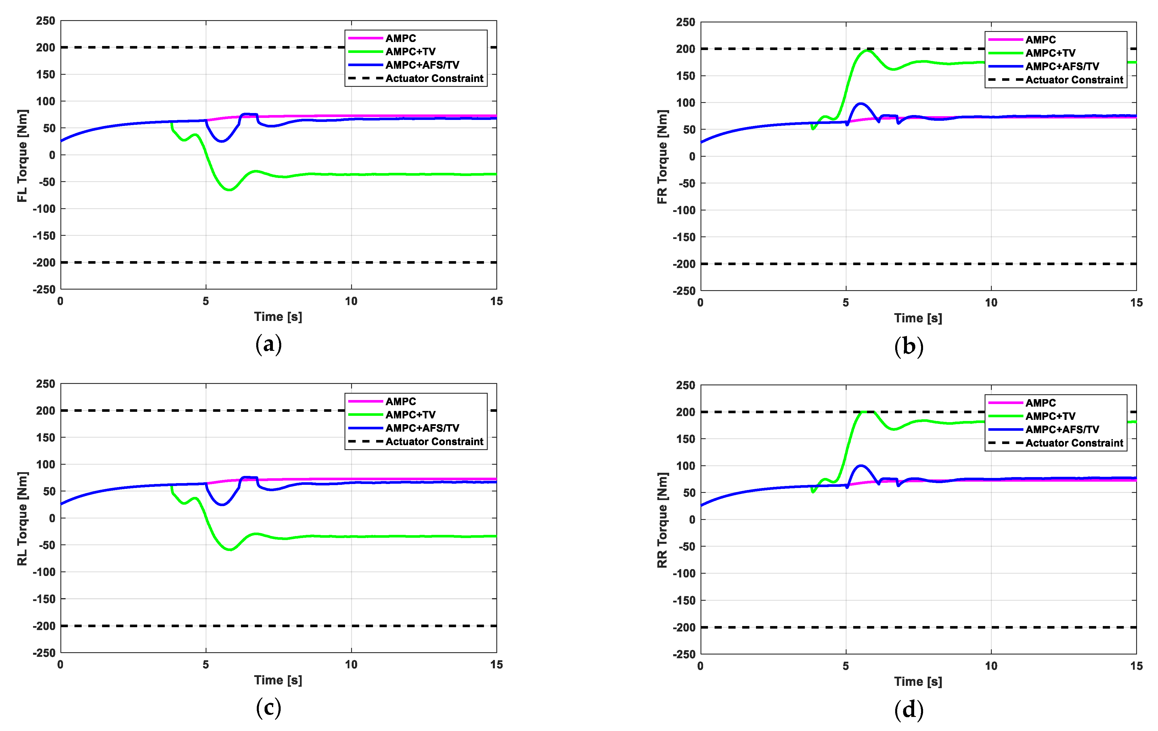
4.2.2. Torque Vectoring Control

In this design, the TV control logic was designed so that it comes into play only when the steering effort from AFS is not enough to produce the command yaw moment from the upper chassis controller. Equation (29) shows the amount of yaw moment that TV provides.
M T V = M B 2 C f l f Δ δ A F S
Unlike the AFS-generated yaw moment for front steering, the TV controller generates a yaw moment with different longitudinal forces at four wheels. The control variables of TV can be defined as below.
u T V = [ Δ F x f l Δ F x f r Δ F x r l Δ F x r r ]
An electric vehicle powered by four IWMs can realize any combination of longitudinal forces at its four wheels; even a combination of traction at some wheels and braking at others is possible. This flexibility enables the system to consider different performance aspects at the same time. To find u T V in Equation (30), a weighted least square problem was formulated as below.
m i n   u T V [ | | W u u T V | | 2 + | | W T V ( C T V u T V M T V ) | | 2 + | | W a ( C a u T V d a ) | | 2 ]
s u b j e c t   t o ( F x i j + Δ F x i i ) r e f f | T m a x | ,         i = f , r     j = l , r
In Equation (31a), W u ,   W T V , and W a are the weighting factors, and C T V and C a are the coefficient vectors. These five variables are explained later in this section. The parameter r e f f is the effective radius of the tire, and T m a x is the maximum torque that each IWM can produce.
The three terms in the cost function of Equation (31a) are explained below. The first term ( | | W u u T V | | 2 ) prevents the longitudinal tire forces from becoming too large. W u is the 4 × 4 matrix in Equation (32). Here, F z (   ) is the vertical force on each tire. The equation implies that the TV controller allows a larger longitudinal force on tires that are subjected to a larger vertical force.
W u = d i a g [ 1 F z f l   1 F z f r   1 F z r l   1 F z r r ]
The second term in Equation (31a) ( | | W T V ( C T V u T V M T V ) | | 2 ) calculates the longitudinal force at each tire to generate M T V in Equation (29). Equation (33) shows the total yaw moment due to the three control efforts: the longitudinal tire forces from the TV controller in Equation (30), Δ δ A F S from the AFS controller in Equation (28), and δ f from the AD controller in Equation (12).
M t o t = l f ( Δ F x f l + Δ F x f r ) sin ( δ f + Δ δ A F S ) + t 2 ( Δ F x f r Δ F x f l ) cos ( δ f + Δ δ A F S ) + t 2 ( Δ F x r r Δ F x r l )
Equation (34) defines C T V from the above equation. Note that C T V is constant, since the TV controller comes after the AD controller and the AFS controller in sequence (see Figure 3).
C T V = [ t 2 cos ( δ f + Δ δ A F S ) + l f sin ( δ f + Δ δ A F S ) t 2 cos ( δ f + Δ δ A F S ) + l f sin ( δ f + Δ δ A F S ) t 2 t 2 ]
W T V in Equation (31a) is a scalar weight that determines the relative importance of the three terms in the cost function. It is a function of the vertical tire forces as defined in Equation (35); it changes consistently with W u when the load balance on the vehicle varies.
W T V = 1.3 F z f l + F z f r + F z r l + F z r r
The third term in Equation (31a) ( | | W a ( C a u T V d a ) | | 2 ) calculates the longitudinal force at each tire Δ F x (   ) in order to meet the desired acceleration in Equation (7). The coefficient vector C a and the constant d a are computed from Equation (5a) by replacing x ¨ with a d e s and by taking into account the three control efforts: δ f from AD, Δ δ A F S from AFS, and Δ F x (   ) from TV. This results in Equation (36).
F y f l sin ( δ f + Δ δ A F S ) + F y f r sin ( δ f + Δ δ A F S ) m γ v y + m a d e s   = cos ( δ f + Δ δ A F S ) ( F x f l + Δ F x f l ) + cos ( δ f + Δ δ A F S ) ( F x f r + Δ F x f r ) + ( F x r l + Δ F x r l ) + ( F x r r + Δ F x r r )
From the above equation, C a and d a can be formulated as in Equation (37a,b).
C a = [ cos ( δ f + Δ δ A F S ) cos ( δ f + Δ δ A F S ) 1 1 ]
d a = F y f l sin ( δ f + Δ δ A F S ) + F y f r sin ( δ f + Δ δ A F S ) m γ v y + m a d e s cos ( δ f + Δ δ A F S ) ( F x f l + F x f r ) F x r l F x r r
From the same reasoning used for finding W T V , the weight W a for achieving a d e s is formulated as in Equation (38). In this way, all three weights W u , W T V , and W a change in harmony with the vertical tire forces, directly affecting the frictional tire forces.
W a = 5 F z f l + F z f r + F z r l + F z r r
Once the longitudinal tire forces Δ F x (   ) are computed by the TV logic, Equation (6) converts them into the corresponding torques Δ T w (   ) which become the command torques for the four IWMs.
Δ T w i j = r e f f ( F x i j + Δ F x i j ) + J w ω ˙ i j T w i j ,     i = f , r     j = l , r

5. Simulation

This section presents the results of the simulation that was conducted to validate the performance of the integrated AD control system of this paper. The three scenarios consist of a double lane change, a high-speed circle entry, and a single lane change; the latter scenario was performed to verify the closed-loop system’s stability through a phase plane trajectory.
This control system (hereafter called AMPC + AFS/TV) was compared with other control systems: “AMPC + TV”, “AMPC”, and “pure pursuit”. “AMPC + TV” consists of an AD controller with AMPC and a TV chassis controller, “AMPC” performs AD control with AMPC without any chassis control, and “pure pursuit” performs only AD control with the pure pursuit algorithm [2].
The vehicle dynamics were implemented using CarMaker, and the EV Tesla-S model in CarMaker was used [33] as the vehicle model. The control system was implemented with MATLAB/Simulink [34]. Table 1 shows the vehicle model parameter values.

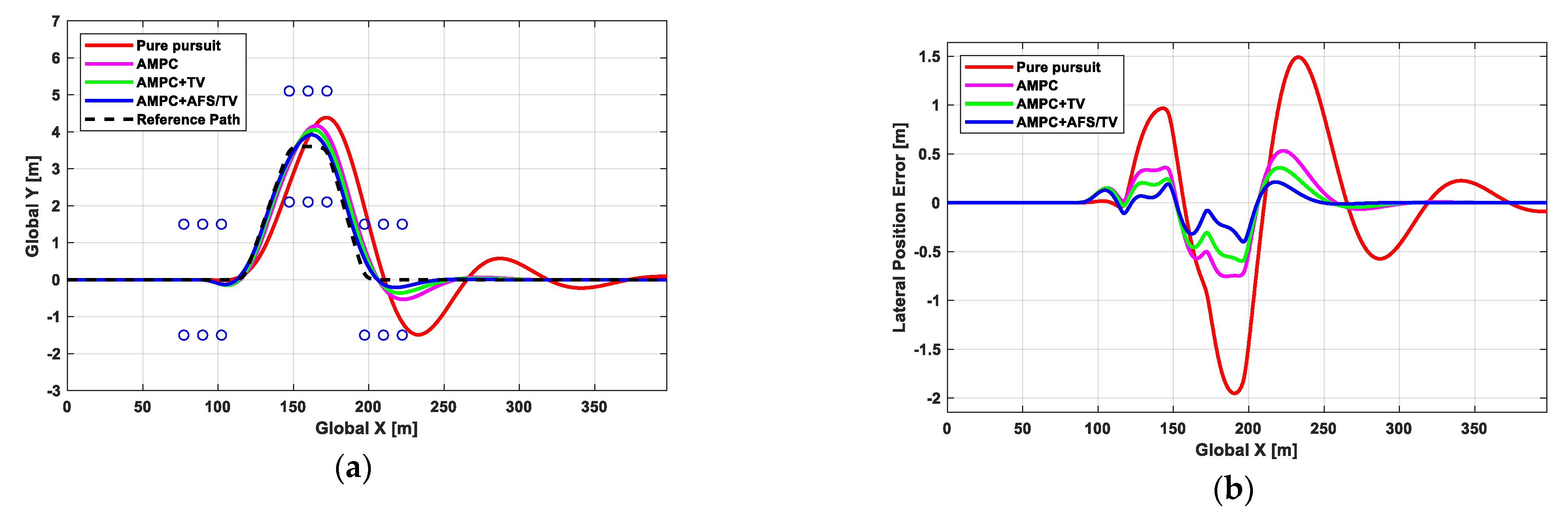
5.1. Scenario 1: Double Lane Change

Figure 5 is the double lane change scenario of ISO-3888 that was used for the simulation described in this section. The solid line is the global path that the autonomous vehicle needs to follow. The road friction coefficient was set to 0.8, and the target vehicle speed was set to 90 km/h or 25 m/s. This scenario presents a rather severe condition for lateral control, since the lane changes must be made in 1.2 s with an in-between dwell time of only 1 s.
Figure 6 shows the path tracking performance of the four different controllers. Among the four, AMPC + AFS/TV gives the best tracking capability with the least overshoot and the quickest response time. The maximum magnitudes of lateral position error from Figure 6b are 1.95 m for pure pursuit, 0.75 m for AMPC, 0.59 m for AMPC + TV, and 0.4 m for AMPC + AFS/TV.
Figure 7 shows the variables related to the vehicle’s lateral stability: the yaw rate error and the sideslip angle. The yaw rate error maximums are 7.70 deg/s for pure pursuit, 6.93 deg/s for AMPC, 6.14 deg/s for AMPC + TV, and 5.70 deg/s for AMPC + AFS/TV. Figure 7b shows the time history of the side-slip angle. The side-slip angle maximums are 0.74 deg for pure pursuit, 0.78 deg for AMPC, 0.66 deg for AMPC + TV, and 0.63 deg for AMPC + AFS/TV. In a region around 5 s in Figure 7b, pure pursuit appears to be better than the other schemes, but careful examination shows that this is only because pure pursuit’s response is slow. Note that AMPC + AFS/TV converges to the final value more quickly than any other controller.
Figure 8 shows the control efforts by the different controllers to accomplish the double lane change maneuver. Figure 8a shows the front steer angle. Among the four controllers, AMPC + TV produces the smallest steering angle maximum; this is because this controller does not use any additional steering angle other than the one required by the AD controller for path tracking. The next smallest steering angle is achieved by AMPC + AFS/TV.
Figure 8b compares the desired yaw moment computed by the TV logic in the AMPC + TV and AMPC + AFS/TV controllers. This figure clearly shows the advantage of integrating AFS with TV in the chassis controller. The TV control effort is significantly reduced to nearly one-third that of TV alone, which implies less energy consumption by the motors and more friction margin within the road–tire contact patch. This increased road friction margin can enable emergency maneuvers where dynamic road friction is pushed to the limit.
Figure 9 shows the torque of each IWM for the different controllers. The DC offset of 50 Nm at each wheel is the torque required to maintain a constant speed in the presence of disturbances such as air drag and rolling resistance. The dashed lines in each figure represent the maximum torque that each motor can produce.
As can be seen in Figure 9b, AMPC + AFS/TV uses much less torque than AMPC + TV to carry out the same double lane change maneuver. The graphs for AMPC + TV show that the torques at the front-left and rear-left tires saturate to their limits for an interval, but this does not occur for AMPC + AFS/TV. In AMPC + TV, the torque profiles for both sides are nearly out of phase, which means that the TV controller generates yaw motion by traction on one side and braking on the other side to maintain vehicle stability without losing speed. AMPC shows nonzero torque variations because the AD controller implements speed control as well as path tracking.

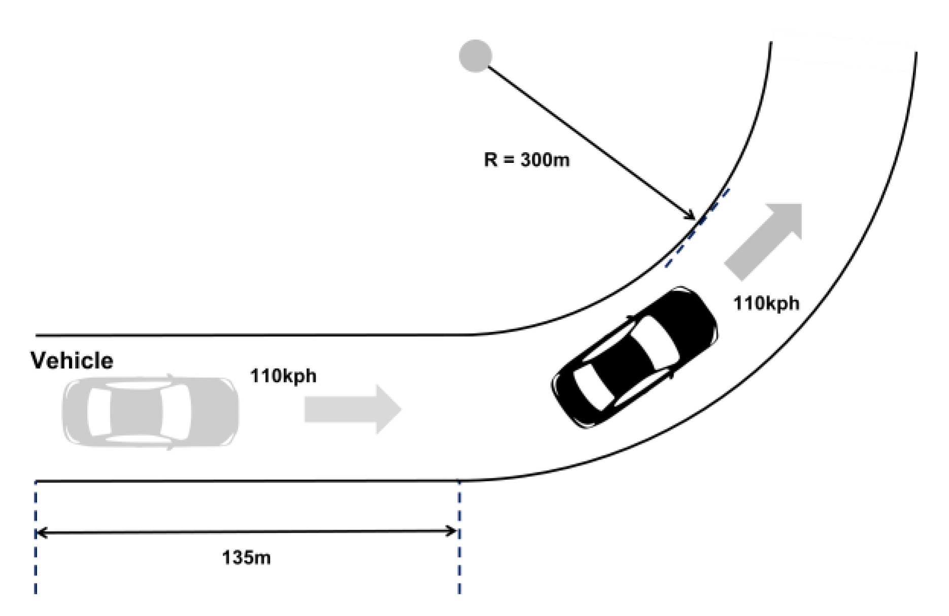
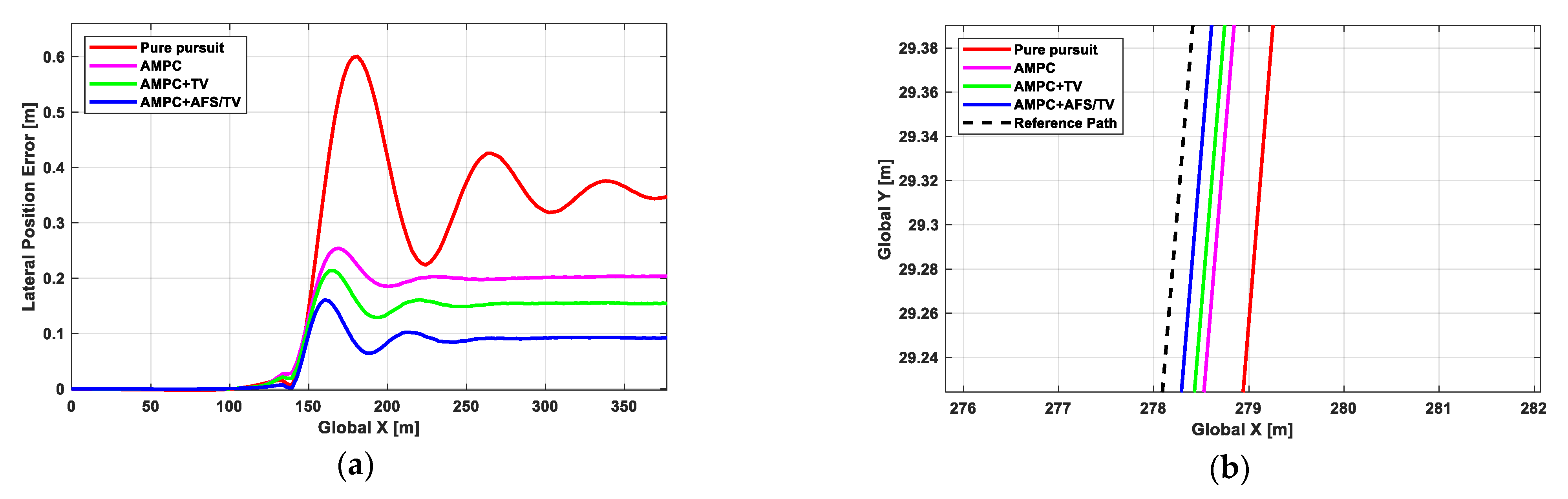
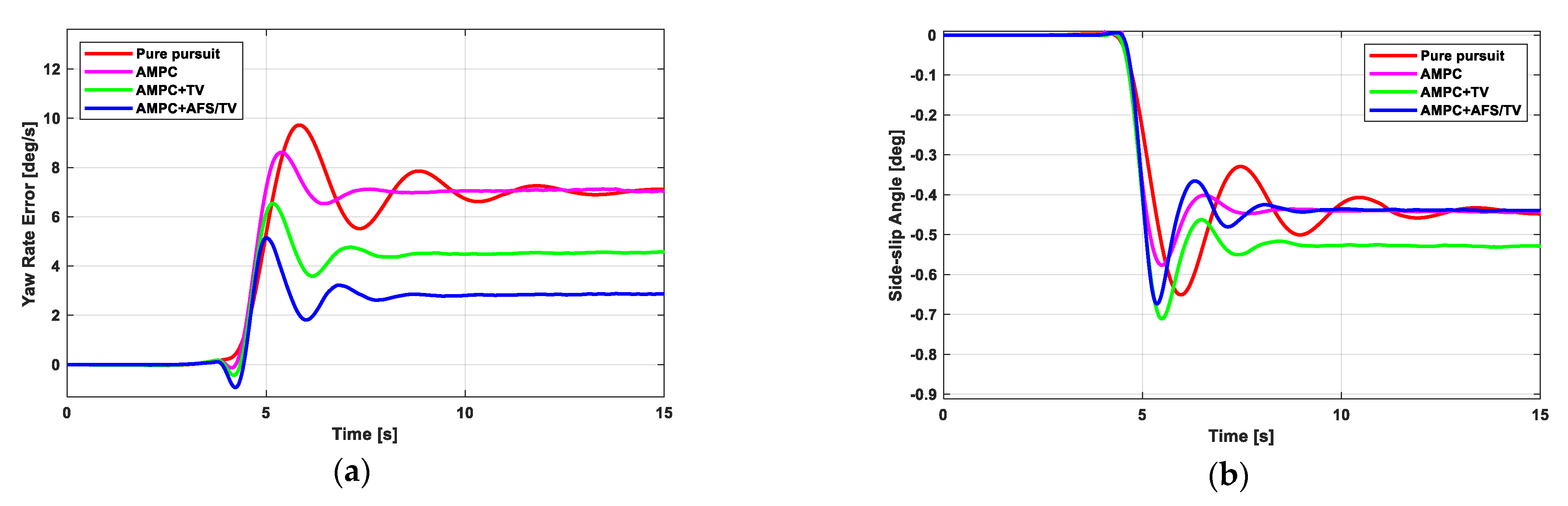
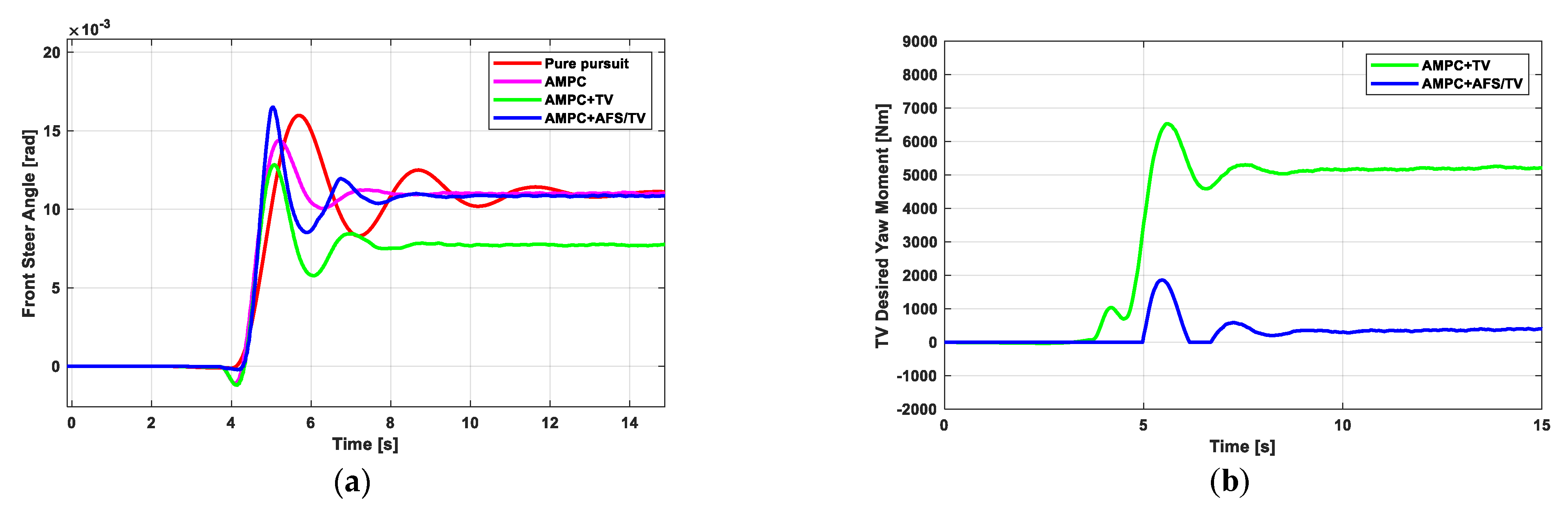
5.2. Scenario 2: High-Speed Circle Entry

Figure 10 illustrates a scenario for the evaluation of transients when entering a curve and steady-state performance in curve driving. This scenario is composed of a 135 m long straight road that becomes curved with a radius R of 300 m.
Figure 11 shows the path tracking performance for entering a circle at high speed. In AMPC + AFS/TV’s overshoot and steady-state lateral position, the error was the smallest of all. The maximum value of the lateral position error was 0.60 m for pure pursuit, 0.25 m for AMPC, 0.20 m for AMPC + TV, and 0.14 m for AMPC + AFS/TV. The steady-state lateral position error was 0.35 m for pure pursuit, 0.20 m for AMPC, 0.15 m for AMPC + TV, and 0.09 m for AMPC + AFS/TV.
Figure 12 shows the yaw rate error and side-slip angle related to vehicle stability. Figure 12a shows that AMPC + TV and AMPC + AFS/TV applied additional chassis control and generated a smaller yaw rate error than the other controllers. The yaw rate error of AMPC + TV and AMPC + AFS/TV was smaller than that of other controllers because the upper controller generated the yaw moment considering the current yaw rate. Figure 12b shows that AMPC + TV’s maximum side-slip angle increased by 0.14 degrees compared with AMPC. This is because an additional yaw moment occurred to reduce the lateral position error when entering the curve.
Figure 13 shows the control efforts by the different controllers. Figure 13a shows that the front steering angle was the smallest in AMPC + TV. This is because the lateral position error was reduced due to the TV action to decrease the lateral position error, and the AMPC performed steering control based on the reduced lateral position error. On the other hand, AMPC + AFS/TV’s front steering angle was similar to that of other controllers in steady state because it used AFS and TV control. Figure 12b shows that AMPC + TV generated a TV desired yaw moment earlier than AMPC + AFS/TV. The magnitude of the desired yaw moment in AMPC + TV was also larger than that of AMPC + AFS/TV. This is because AMPC + AFS/TV used AFS control before TV control.
Figure 14 shows the torque distributed to each wheel. An offset of about 60 Nm occurred to maintain a constant speed in the presence of disturbances. As shown in Figure 13b, the yaw moment of AFS/TV was large and reached the IWM limit. This should be avoided as it cannot generate more motor force and overloads the motor. On the other hand, since AMPC + AFS/TV generated an additional yaw moment from AFS, AMPC + AFS/TV reduced the amount of torque distributed to each wheel. Torque distribution occurred earlier in AMPC + TV than in MPC + AFS/TV, because AMPC + AFS/TV generated the desired yaw moment earlier.

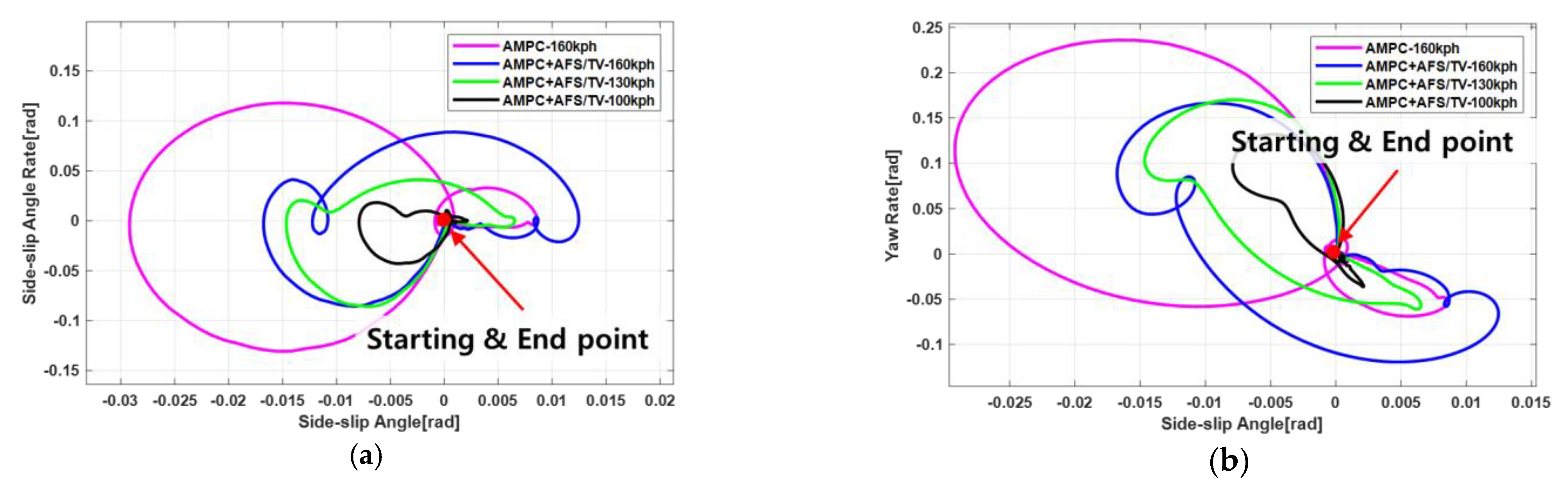
5.3. Scenario 3: Single Lane Change (for Stability Analysis)

Phase plane analysis is a method of confirming system characteristics or stability. The phase plane of a side-slip angle can predict lateral vehicle stability [35,36,37]. A single lane change was performed at speeds of 100 kph, 130 kph, and 160 kph to verify the stability of the closed-loop system of AMPC + AFS/TV. Since Scenario 1 and Scenario 2 demonstrated the system’s performance, this scenario focused on its stability using the side-slip angle phase plane.
Figure 15 shows the phase plane of AMPC + AFS/TV at speeds of 100, 130, and 160 kph, and the phase plane of AMPC at 160 kph. In each phase plane, the state variables were located at the origin. As the speed increased, the trajectory of each state variable increased. However, since the vehicle entered a stable state by completing the single lane change, the state variables converged back at their origin. In AMPC + AFS/TV with a speed of 160 kph, the trajectory of state variables was in a smaller range than that of AMPC. This was because when generating an additional yaw moment, the yaw rate error, which is one of the vehicle’s stability indicators, was used as a controlling factor. The closed-loop system is stable up to a speed of 160 kph.

6. Conclusions

This paper proposes an integrated AD control system design for an autonomous vehicle with an independent IWM at each wheel. The system consists of an AD controller and a chassis controller that are functionally integrated to improve vehicle stability as well as path tracking performance. The AD controller implements longitudinal/lateral path tracking control using PI control and AMPC. The chassis controller is composed of two lateral control units: the AFS control and the TV control. They jointly find the yaw moment that maintains vehicle stability using slide-mode control; AFS is prioritized over TV to enhance the safety margin and save energy.
Validation was performed by simulating a double lane change, a high-speed circle entry, and a single lane change scenario. The control system of this paper was compared with three other control systems. The proposed system gave the best tracking performance with the least overshoot and the quickest response time. For vehicle stability as represented by the yaw rate error, the control system of this paper produced the smallest maximum and fastest convergence to a final value. The simulation results also showed the advantage of the chassis controller’s integration scheme: less energy consumption and more safety margin, which can be valuable in emergency maneuvers.
Finally, the contributions of this study can be summarized as follows. There have been many studies for improving vehicle stability in lateral chassis control and also many studies for improving path tracking performance in AD, but there have been few studies that consider both at the same time. As AD technology advances, both objectives should be considered together, since they both contribute significantly to the safety of the autonomous vehicle but often affect each other in conflicting ways. To address this problem, an integrated AD control system that consists of the AD controller and the chassis controller has been developed in this study. The proposed system adopted the AMPC method and the SMC method, since it was found that their combination could effectively minimize the lateral position error and the yaw rate error at the same time. The proposed algorithm was tested on various scenarios, and the simulation results verified that the proposed algorithm could significantly improve both path tracking capability and vehicle stability compared with other control systems.
Potential drawbacks of the proposed algorithm may include: (1) the algorithm requires many complex computations, and this may cause a given sampling interval, which is usually 10 msec for most chassis controls, to be skipped, and (2) any non-deterministic optimization process can always fail to converge; the proposed algorithm contains such problems. Regarding the first issue, it is worth noting that the limits of ECU computing power are rapidly increasing as vehicle control technology advances from chassis control to AD requirements for handling massive amounts of data coming from environmental sensors. As for the second issue, the optimization of the proposed algorithm is computed at every sample, and there can be many strategies to find an alternative solution when optimization convergence failure occurs such as using the solution computed in the previous step. Future study plans include the implementation of the proposed algorithm on a test vehicle to tackle practical issues such as the ones mentioned above.

Author Contributions

Conceptualization, T.A.; methodology, T.A.; software, T.A., Y.L.; validation, T.A., Y.L.; investigation, T.A.; writing—original draft preparation, T.A.; writing—review and editing, K.P.; visualization, T.A.; supervision, K.P.; All authors have read and agreed to the published version of the manuscript.

Funding

This research received no external funding.

Acknowledgments

This work was supported by the Industrial Strategic Technology Development Program (Project Title: Development of Safety Evaluation Methods for Environment Perception Modules and Fail-operation Technologies for Autonomous Vehicles, Project No.: 10062448) funded by the Ministry of Trade, Industry & Energy (MOTIE, Korea). This research was supported by Innovative Incubation Center for Autonomous xEV Technology through the National Research Foundation of Korea(NRF) funded by the Ministry of Education (5199990814084) and the Transportation Logistics Development Program (20TLRP-B147674-03) funded by the Ministry of Land, Infrastructure and Transport (MOLIT), Korea.

Conflicts of Interest

The authors declare no conflict of interest.

Nomenclature

Mvehicle mass
l f distance from center of gravity to the front axle
l r distance from center of gravity to the rear axle
v x longitudinal vehicle speed
γ yaw rate
β side-slip angle
I z vehicle moment of inertia about z-axis
M B the yaw moment acting on the vehicle body
δ f front steer angle
Δ δ A F S front steer angle generated by AFS
α f wheel slip angle of front tire
α r wheel slip angle of rear tire
C f cornering stiffness of front tire
C r cornering stiffness of rear tire
F x f l longitudinal tire force on front left tire
F x f r longitudinal tire force on front right tire
F x r l longitudinal tire force on rear left tire
F x r r longitudinal tire force on rear right tire
F y f l lateral tire force on front left tire
F y f r lateral tire force on front right tire
F y r l lateral tire force on rear left tire
F y r r lateral tire force on rear right tire
F z f l vertical tire force on front left tire
F z f r vertical tire force on front right tire
F z r l vertical tire force on rear left tire
F z r r vertical tire force on rear right tire
J w rotational moment of inertia of each wheel
Ttrack width
T w f l wheel torque transmitted to the front left
T w f r wheel torque transmitted to the front right
T w r l wheel torque transmitted to the rear left
T w r r wheel torque transmitted to the rear right
g gravitational acceleration
μ road friction coefficient
r e f f effective radius of the tire
T m a x maximum torque of in-wheel motor
Δ F x f l longitudinal tire force on front left by TV
Δ F x f r longitudinal tire force on front right by TV
Δ F x r l longitudinal tire force on rear left by TV
Δ F x r r longitudinal tire force on rear right by TV
Δ T w f l in-wheel motor torque on front left by TV
Δ T w f r in-wheel motor torque on front right by TV
Δ T w r l in-wheel motor torque on rear left by TV
Δ T w r r in-wheel motor torque on rear right by TV

References

  1. Andersen, H.; Chong, Z.J.; Eng, Y.H.; Pendleton, S.; Ang, M.H. Geometric path tracking algorithm for autonomous driving in pedestrian environment. In Proceedings of the 2016 IEEE International Conference on Advanced Intelligent Mechatronics (AIM), Banff, AB, Canada, 12–15 July 2016; pp. 1669–1674. [Google Scholar]
  2. Giesbrecht, J.; Mackay, D.; Collier, J.; Verret, S. Path tracking for unmanned ground vehicle navigation. DRDC Suffield TM 2005. Technical Memorandum 2005-224. [Google Scholar]
  3. Snider, J.M. Automatic Steering Methods for Autonomous Automobile Path Tracking; Robotics Institute: Pittsburgh, PA, USA, 2009; Tech. Rep. CMU-RITR-09-08. [Google Scholar]
  4. Thrun, S.; Montemerlo, M.; Dahlkamp, H.; Stavens, D.; Aron, A.; Diebel, J.; Fong, P.; Gale, J.; Halpenny, M.; Hoffmann, G.; et al. Stanley: The robot that won the DARPA Grand Challenge. J. Field Robot. 2006, 23, 661–692. [Google Scholar] [CrossRef]
  5. Nguyen, A.-T.; Sentouh, C.; Zhang, H.; Popieul, J.-C. Fuzzy static output feedback control for path following of autonomous vehicles with transient performance improvements. Proc. IEEE Trans. Intell. Transp. Syst. 2019, 21, 3069–3079. [Google Scholar] [CrossRef]
  6. Nguyen, A.-T.; Rath, J.; Guerra, T.-M.; Palhares, R.; Zhang, H. Robust set-invariance based fuzzy output tracking control for vehicle autonomous driving under uncertain lateral forces and steering constraints. In Proceedings of the 2020 IEEE International Conference on Fuzzy Systems (FUZZ-IEEE), Glasgow, UK, 19–24 July 2020. [Google Scholar]
  7. Mashadi, B.; Mahmoodi-K, M.; Kakaee, A.H.; Hosseini, R. Vehicle path following control in the presence of driver inputs. Proc. Inst. Mech. Eng. Part K J. Multi-Body Dyn. 2013, 227, 115–132. [Google Scholar] [CrossRef]
  8. Hang, P.; Chen, X.; Luo, F.; Fang, S. Robust Control of a Four-Wheel-Independent-Steering Electric Vehicle for Path Tracking. SAE Int. J. Veh. Dyn. Stab. NVH 2017, 1, 307–316. [Google Scholar] [CrossRef]
  9. Burke, M. Path-following control of a velocity constrained tracked vehicle incorporating adaptive slip estimation. In Proceedings of the 2012 IEEE International Conference on Robotics and Automation, Saint Paul, MN, USA, 14–18 May 2012; pp. 97–102. [Google Scholar]
  10. Sun, C.; Zhang, X.; Zhou, Q.; Tian, Y. A Model Predictive Controller with Switched Tracking Error for Autonomous Vehicle Path Tracking. IEEE Access 2019, 7, 53103–53114. [Google Scholar] [CrossRef]
  11. Ji, J.; Khajepour, A.; Melek, W.W.; Huang, Y. Path Planning and Tracking for Vehicle Collision Avoidance Based on Model Predictive Control With Multiconstraints. IEEE Trans. Veh. Technol. 2017, 66, 952–964. [Google Scholar] [CrossRef]
  12. Yoshida, H.; Shinohara, S.; Nagai, M. Lane change steering manoeuvre using model predictive control theory. Veh. Syst. Dyn. 2008, 46, 669–681. [Google Scholar] [CrossRef]
  13. Nam, H.; Choi, W.; Ahn, C. Model predictive control for evasive steering of an autonomous vehicle. Int. J. Automot. Technol. 2019, 20, 1033–1042. [Google Scholar] [CrossRef]
  14. Gao, Y.; Lin, T.; Borrelli, F.; Tseng, E.; Hrovat, D. Predictive control of autonomous ground vehicles with obstacle avoidance on slippery roads. In Proceedings of the ASME 2010 Dynamic Systems and Control Conference, American Society of Mechanical Engineers Digital Collection, Cambridge, MA, USA, 12–15 September 2010; pp. 265–272. [Google Scholar]
  15. Rafaila, R.C.; Livint, G. Nonlinear model predictive control of autonomous vehicle steering. In Proceedings of the 2015 19th International Conference on System Theory, Control and Computing (ICSTCC), Cheile Gradistei, Romania, 14–16 October 2015; pp. 466–471. [Google Scholar]
  16. Findeisen, R.; Allgöwer, F. An introduction to nonlinear model predictive control. In Proceedings of the 21st Benelux Meeting on Systems and Control, Eindhoven, The Netherlands, 19–21 March 2002; pp. 119–141. [Google Scholar]
  17. Lin, F.; Chen, Y.; Zhao, Y.; Wang, S. Path tracking of autonomous vehicle based on adaptive model predictive control. Int. J. Adv. Robot. Syst. 2019, 16, 1729881419880089. [Google Scholar] [CrossRef]
  18. Ercan, Z.; Gokasan, M.; Borrelli, F. An adaptive and predictive controller design for lateral control of an autonomous vehicle. In Proceedings of the 2017 IEEE International Conference on Vehicular Electronics and Safety (ICVES), Vienna, Austria, 27–28 June 2017; pp. 13–18. [Google Scholar]
  19. Petersson, I.; Risö, J. Automotive Path Following Using Model Predictive Control. Master’s Thesis, Chalmers University of Technology, Göteborg, Sweden, 2014. [Google Scholar]
  20. Yim, S.; Kim, S.; Yun, H. Coordinated control with electronic stability control and active front steering using the optimum yaw moment distribution under a lateral force constraint on the active front steering. Proc. Inst. Mech. Eng. Part D J. Automob. Eng. 2016, 230, 581–592. [Google Scholar] [CrossRef]
  21. Zhang, J.; Li, J. Integrated vehicle chassis control for active front steering and direct yaw moment control based on hierarchical structure. Trans. Inst. Meas. Control 2019, 41, 2428–2440. [Google Scholar] [CrossRef]
  22. Cho, W.; Yoon, J.; Kim, J.; Hur, J.; Yi, K. An investigation into unified chassis control scheme for optimised vehicle stability and manoeuvrability. Veh. Syst. Dyn. 2008, 46, 87–105. [Google Scholar] [CrossRef]
  23. Kang, J.; Heo, H. Control Allocation based Optimal Torque Vectoring for 4WD Electric Vehicle; 0148-7191; SAE Technical Paper: Warrendale, PA, USA, 2012. [Google Scholar]
  24. Ando, N.; Fujimoto, H. Yaw-rate control for electric vehicle with active front/rear steering and driving/braking force distribution of rear wheels. In Proceedings of the 2010 11th IEEE International Workshop on Advanced Motion Control (AMC), Nagaoka, Niigata, Japan, 21–24 March 2010; pp. 726–731. [Google Scholar]
  25. Osborn, R.P.; Shim, T. Independent control of all-wheel-drive torque distribution. Veh. Syst. Dyn. 2006, 44, 529–546. [Google Scholar] [CrossRef]
  26. Zhang, X.; Göhlich, D.; Zheng, W. Karush–Kuhn–Tuckert based global optimization algorithm design for solving stability torque allocation of distributed drive electric vehicles. J. Frankl. Inst. 2017, 354, 8134–8155. [Google Scholar] [CrossRef]
  27. Shino, M.; Nagai, M. Yaw-moment control of electric vehicle for improving handling and stability. JSAE Rev. 2001, 22, 473–480. [Google Scholar] [CrossRef]
  28. Hori, Y. Future vehicle driven by electricity and control-research on four wheel motored “UOT Electric March II”. In Proceedings of the 7th International Workshop on Advanced Motion Control. Proceedings (Cat. No. 02TH8623), Maribor, Slovenia, 3–5 July 2002; pp. 1–14. [Google Scholar]
  29. Abe, M. Vehicle Handling Dynamics: Theory and Application; Butterworth-Heinemann: Burlington, MA, USA, 2015. [Google Scholar]
  30. Rajamani, R. Vehicle Dynamics and Control; Springer: Berlin/Heidelberg, Germany, 2011. [Google Scholar]
  31. Willis, M.J.; Tham, M.T. Advanced Process Control; Department of Chemical and Process Engineering, University of Newcastle upon Tyne; University of Newcastle upon Tyne: Tyne, UK, 1994. [Google Scholar]
  32. Breuer, J.J. Analysis of driver-vehicle-interactions in an evasive manoeuvre-results of’moose test’studies. In Proceedings of the 16th International Technical Conference on the Enhanced Safety of Vehicles, Windsor, ON, Canada, 31 May–4 June 1998. [Google Scholar]
  33. CarMaker. User’s Guide Version 8.0; IPG Automotive: Karlsruhe, Germany, 2019. [Google Scholar]
  34. MathWorks. Simulink User’s Guide; The MathWorks Inc.: Natick, MA, USA, 2018. [Google Scholar]
  35. Zhang, H.; Li, X.-S.; Shi, S.-M.; Liu, H.-F.; Guan, R.; Liu, L. Phase plane analysis for vehicle handling and stability. Int. J. Comput. Intell. Syst. 2011, 4, 1179–1186. [Google Scholar] [CrossRef]
  36. Nguyen, V. Vehicle Handling, Stability, and Bifurcaiton Analysis for Nonlinear Vehicle Models. Master’s Thesis, University of Maryland, Maryland, DC, USA, 2005. [Google Scholar]
  37. Inagaki, S.; Kushiro, I.; Yamamoto, M. Analysis on vehicle stability in critical cornering using phase-plane method. JSAE Rev. 1995, 2, 216. [Google Scholar]
Figure 1. 2 degree of freedom (DOF) vehicle model.
Electronics 10 00144 g001
Figure 2. 7-DOF vehicle model.
Electronics 10 00144 g002
Figure 3. The architecture of the integrated autonomous driving (AD) control system.
Electronics 10 00144 g003
Figure 4. Target path and predicted path of the vehicle.
Electronics 10 00144 g004
Figure 5. Double lane-change scenario.
Electronics 10 00144 g005
Figure 6. (a) Vehicle trajectory and (b) lateral position error.
Electronics 10 00144 g006
Figure 7. (a) Yaw rate error and (b) side-slip angle.
Electronics 10 00144 g007
Figure 8. (a) Front steer angle and (b) desired yaw moment by torque vectoring (TV).
Electronics 10 00144 g008
Figure 9. Independent in-wheel motors (IWM) torque: (a) front-left, (b) front-right, (c) rear-left, and (d) rear-right.
Electronics 10 00144 g009aElectronics 10 00144 g009b
Figure 10. High-speed circle entry scenario.
Electronics 10 00144 g010
Figure 11. (a) Vehicle trajectory and (b) lateral error.
Electronics 10 00144 g011
Figure 12. (a) Yaw rate error and (b) side-slip angle.
Electronics 10 00144 g012
Figure 13. (a) Front steering angle and (b) desired yaw moment by TV.
Electronics 10 00144 g013
Figure 14. Torque distribution: (a) front-left, (b) front-right, (c) rear-left, and (d) rear-right.
Electronics 10 00144 g014
Figure 15. (a) Side-slip angle and side-slip angle rate trajectory and (b) side-slip angle and yaw rate trajectory.
Electronics 10 00144 g015
Table 1. Vehicle model parameters.
ParametersValue
m (kg)2108
C f (N/rad)127,100
C r (N/rad)12,700
I z ( kgm 2 ) 3594.29
l f (m)1.47
l r (m)1.5
t f (m)1.66
t r (m)1.7
Publisher’s Note: MDPI stays neutral with regard to jurisdictional claims in published maps and institutional affiliations.

