
Soil Erosion Prediction Based on Moth-Flame Optimizer-Evolved Kernel Extreme Learning Machine

 ,
, 
Abstract
:1. Introduction
2. Materials and Methods
2.1. Dataset
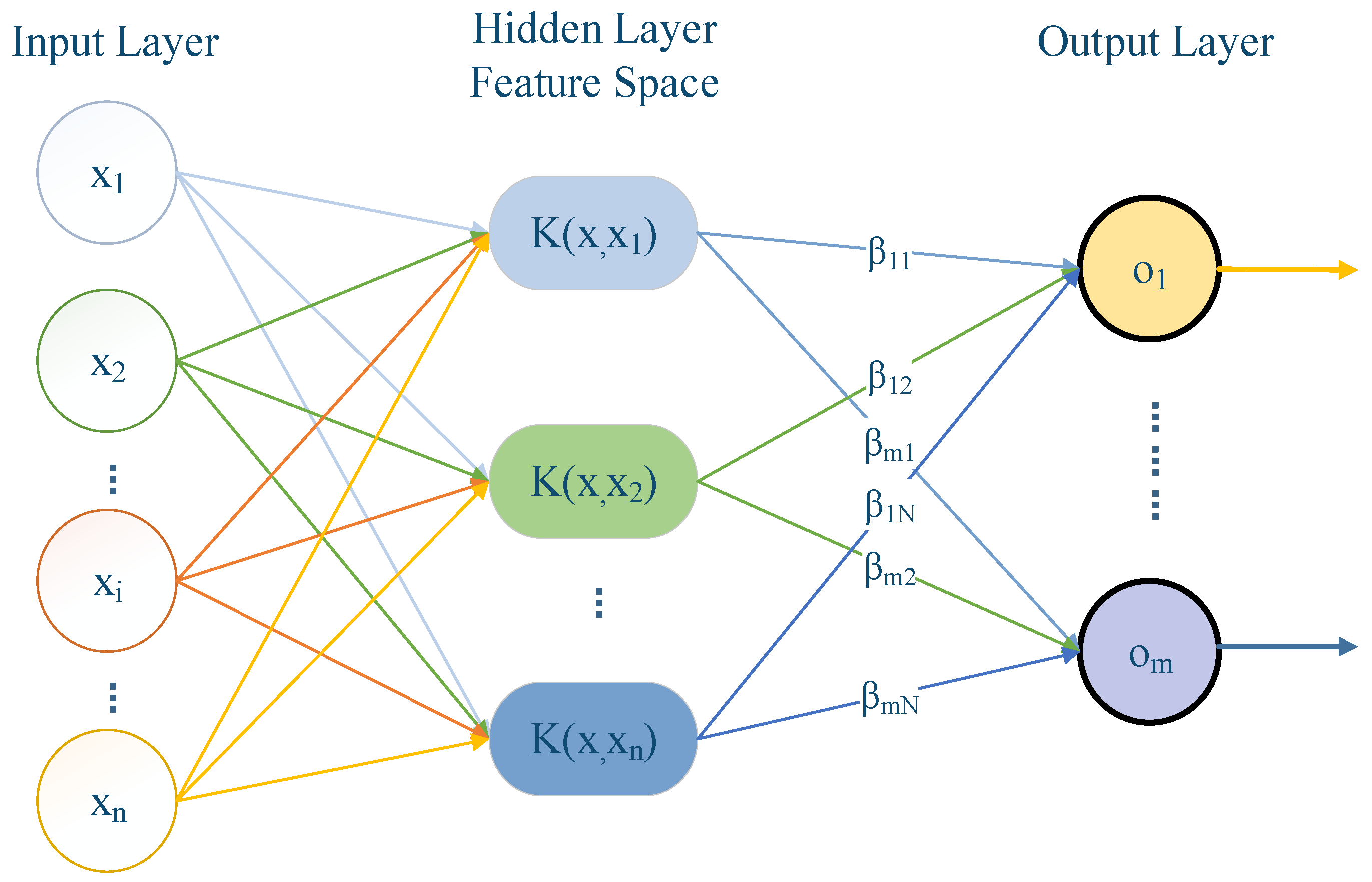
2.2. KELM
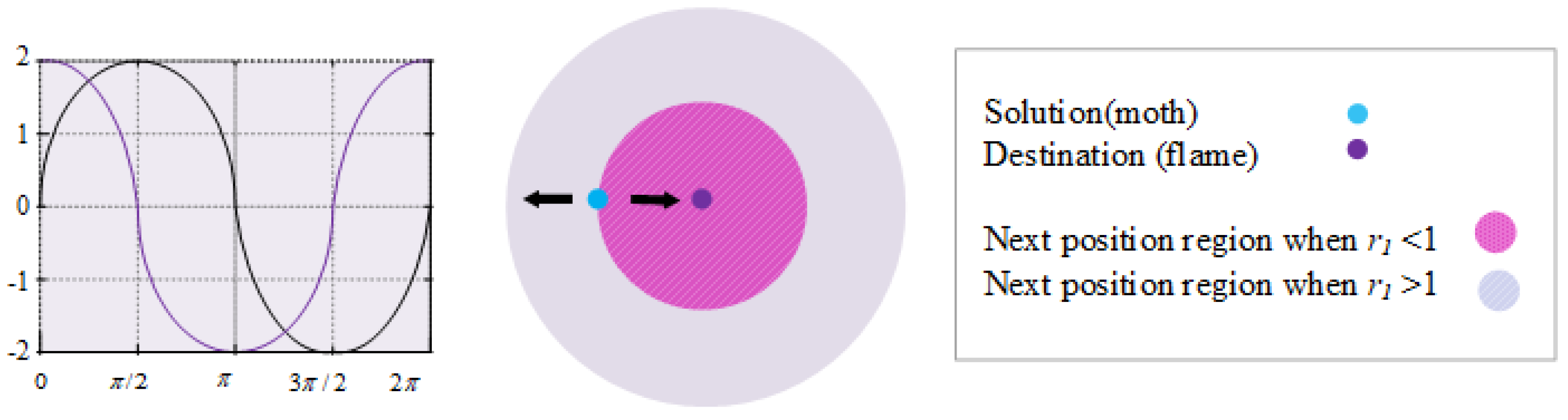
2.3. SMFO
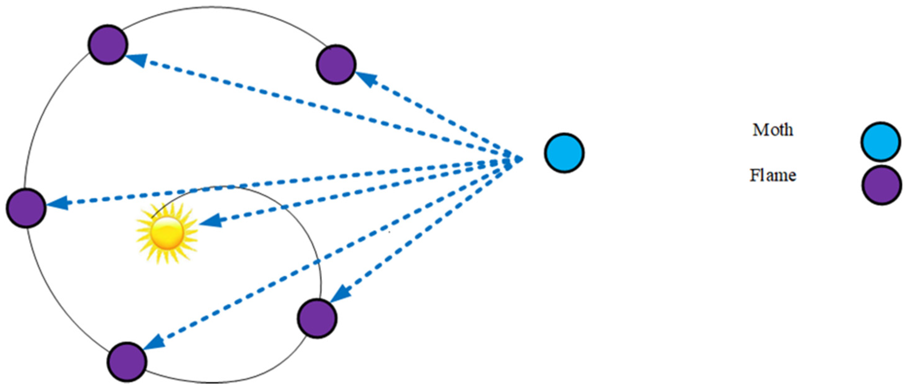
2.3.1. MFO
2.3.2. SMFO
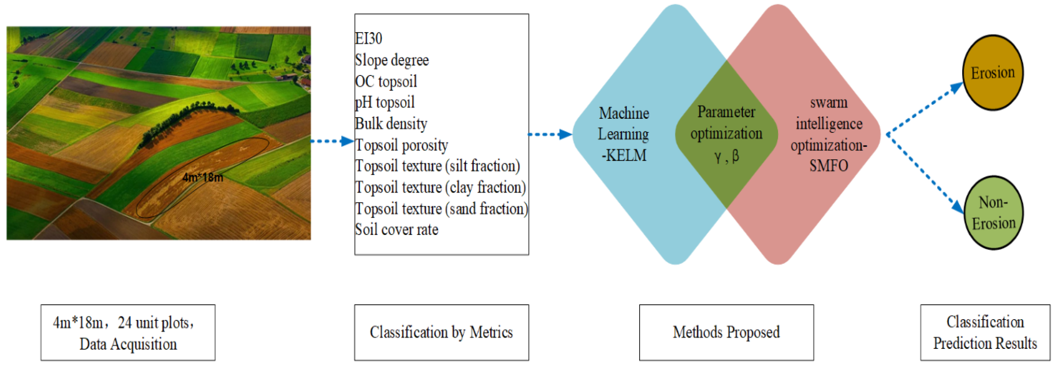
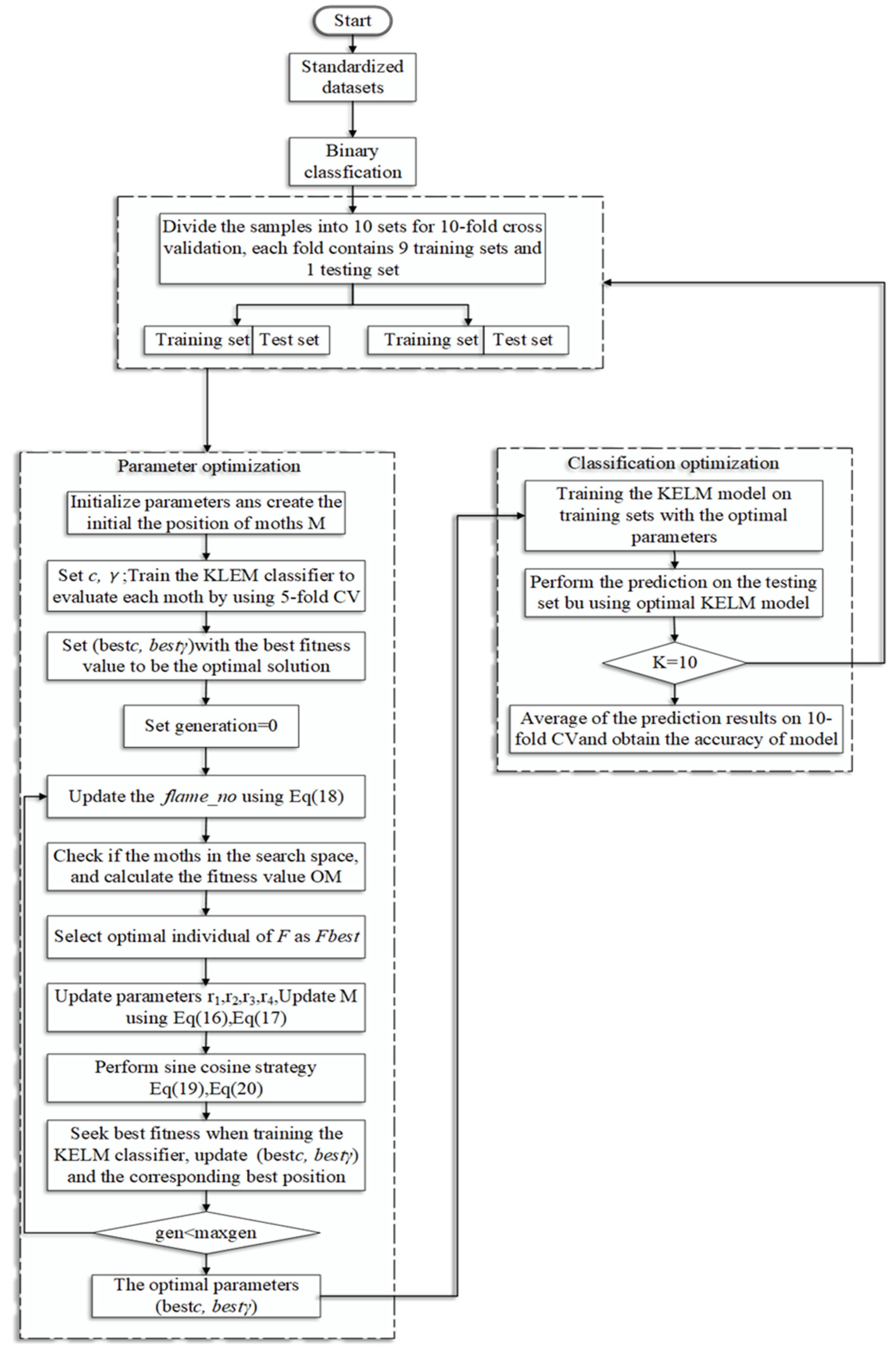
2.4. SMFO-KELM for Soil Erosion Prediction Method
2.5. Experimental Environment
2.6. Measures for Performance Evaluation
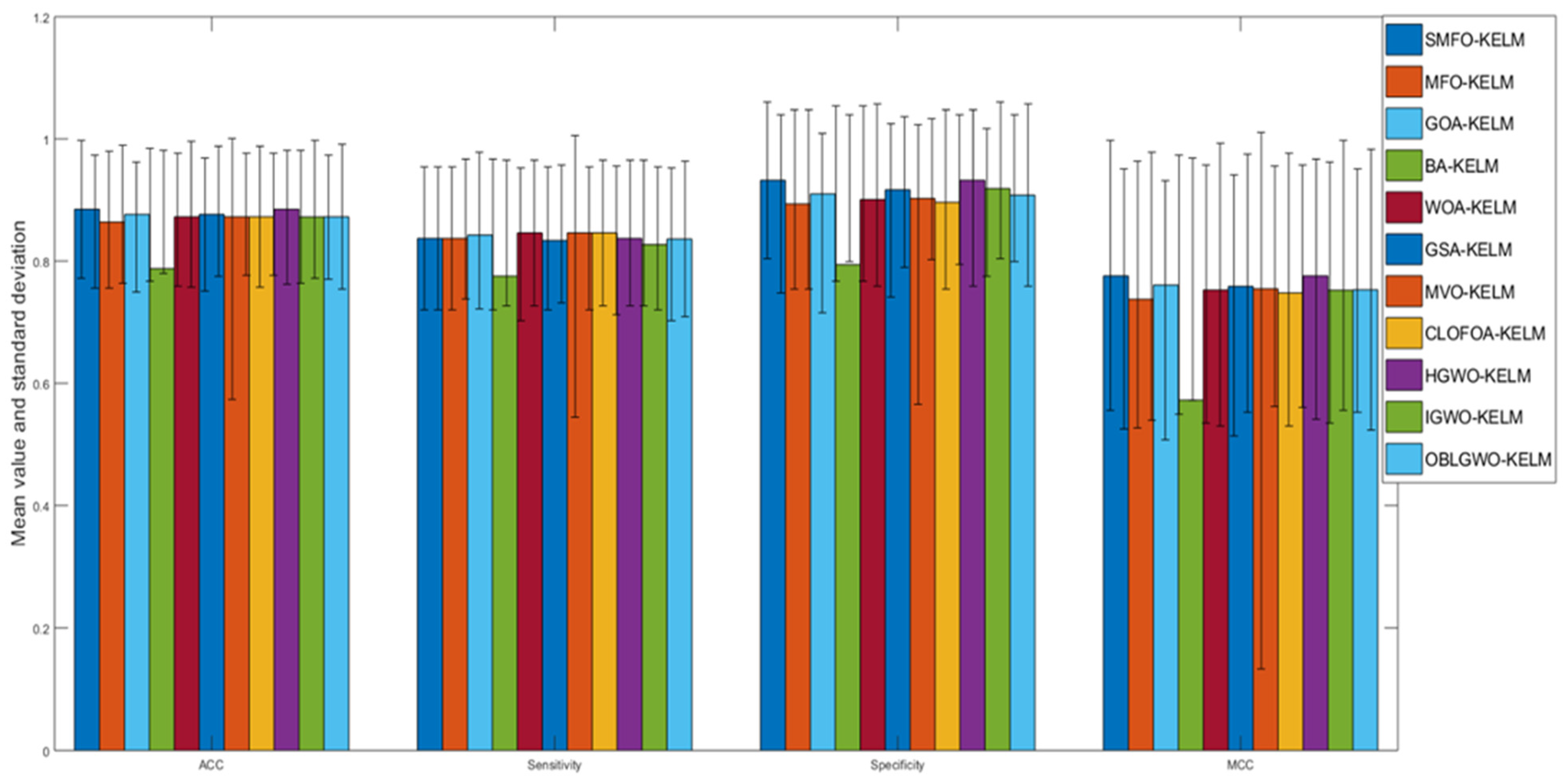
3. Results
4. Conclusions
Author Contributions
Funding
Institutional Review Board Statement
Informed Consent Statement
Data Availability Statement
Acknowledgments
Conflicts of Interest
Appendix A

| No. | a1 | a2 | a3 | a4 | a5 | a6 | a7 | a8 | a9 | a10 | Type |
|---|---|---|---|---|---|---|---|---|---|---|---|
| 1 | 2044.01 | 27.93 | 0.89 | 5.83 | 1.47 | 55.47 | 33.47 | 30.69 | 35.84 | 42.09 | 1 |
| 2 | 975.56 | 29.57 | 1 | 5.8 | 1.46 | 55.26 | 31.35 | 30.43 | 38.21 | 25.91 | 1 |
| 3 | 2044.01 | 28.17 | 1.2 | 6.59 | 1.37 | 51.75 | 34.93 | 27.57 | 37.5 | 60.19 | 1 |
| 4 | 975.56 | 28.17 | 1.2 | 6.59 | 1.37 | 51.75 | 34.93 | 27.57 | 37.5 | 8.98 | 1 |
| 5 | 2044.01 | 29.6 | 1.46 | 6.68 | 1.41 | 53.12 | 33.19 | 20.29 | 46.51 | 54.96 | 1 |
| 6 | 1138.37 | 27.93 | 0.89 | 5.83 | 1.47 | 55.47 | 33.47 | 30.69 | 35.84 | 29.74 | 1 |
| 7 | 975.56 | 28.17 | 1.33 | 6.38 | 1.48 | 55.8 | 34.99 | 24.95 | 40.05 | 18.01 | 1 |
| 8 | 2044.01 | 30.2 | 1.28 | 5.85 | 1.4 | 52.69 | 36.19 | 27.95 | 35.86 | 51.12 | 1 |
| 9 | 2044.01 | 29.57 | 1 | 5.8 | 1.46 | 55.26 | 31.35 | 30.43 | 38.21 | 44.35 | 1 |
| 10 | 1138.37 | 29.6 | 1.46 | 6.68 | 1.41 | 53.12 | 33.19 | 20.29 | 46.51 | 23.59 | 1 |
| 11 | 975.56 | 27.93 | 0.89 | 5.83 | 1.47 | 55.47 | 33.47 | 30.69 | 35.84 | 9.65 | 1 |
| 12 | 976.92 | 28.17 | 1.2 | 6.59 | 1.37 | 51.75 | 34.93 | 27.57 | 37.5 | 5.99 | 1 |
| 13 | 975.56 | 34.77 | 1.42 | 6.72 | 1.37 | 51.87 | 32.73 | 24.33 | 42.93 | 29.9 | 1 |
| 14 | 975.56 | 29.8 | 1.53 | 7.06 | 1.58 | 59.48 | 36.31 | 18.61 | 45.08 | 30.56 | 1 |
| 15 | 3008.93 | 28.63 | 2.39 | 5.2 | 1.44 | 54.49 | 34.73 | 28.89 | 36.37 | 53.9 | 1 |
| 16 | 1270.46 | 28.63 | 2.32 | 5.2 | 1.44 | 54.49 | 34.73 | 28.89 | 36.37 | 10.54 | 1 |
| 17 | 1472.5 | 26.27 | 2.41 | 5.23 | 1.32 | 49.92 | 32.41 | 31.09 | 36.49 | 4.85 | 1 |
| 18 | 2044.01 | 34.77 | 1.42 | 6.72 | 1.37 | 51.87 | 32.73 | 24.33 | 42.93 | 47.03 | 1 |
| 19 | 1138.37 | 29.57 | 1 | 5.8 | 1.46 | 55.26 | 31.35 | 30.43 | 38.21 | 31.98 | 1 |
| 20 | 1270.46 | 28.47 | 2.08 | 5.36 | 1.25 | 47.09 | 31.47 | 34.59 | 33.93 | 12.33 | 1 |
| 21 | 2044.01 | 28.17 | 1.33 | 6.38 | 1.48 | 55.8 | 34.99 | 24.95 | 40.05 | 59.98 | 1 |
| 22 | 975.56 | 30.2 | 1.28 | 5.85 | 1.4 | 52.69 | 36.19 | 27.95 | 35.86 | 26.91 | 1 |
| 23 | 975.56 | 29.6 | 1.46 | 6.68 | 1.41 | 53.12 | 33.19 | 20.29 | 46.51 | 7.65 | 1 |
| 24 | 3008.93 | 26.27 | 2.18 | 5.23 | 1.32 | 49.92 | 32.41 | 31.09 | 36.49 | 60.88 | 1 |
| 25 | 1138.37 | 28.17 | 1.2 | 6.59 | 1.37 | 51.75 | 34.93 | 27.57 | 37.5 | 27.69 | 1 |
| 26 | 2044.01 | 29.8 | 1.53 | 7.06 | 1.58 | 59.48 | 36.31 | 18.61 | 45.08 | 65.48 | 1 |
| 27 | 3008.93 | 28.03 | 2.27 | 5.54 | 1.3 | 49.07 | 33.93 | 30.15 | 35.92 | 44.96 | 1 |
| 28 | 1270.46 | 26.27 | 2.41 | 5.23 | 1.32 | 49.92 | 32.41 | 31.09 | 36.49 | 13.13 | 1 |
| 29 | 975.56 | 34.17 | 0.99 | 5.89 | 1.34 | 50.62 | 34.31 | 35.33 | 30.35 | 22.07 | 1 |
| 30 | 1138.37 | 34.77 | 1.42 | 6.72 | 1.37 | 51.87 | 32.73 | 24.33 | 42.93 | 44.29 | 1 |
| 31 | 685.09 | 28.17 | 1.2 | 6.59 | 1.37 | 51.75 | 34.93 | 27.57 | 37.5 | 14.97 | 1 |
| 32 | 1138.37 | 28.17 | 1.33 | 6.38 | 1.48 | 55.8 | 34.99 | 24.95 | 40.05 | 21.1 | 1 |
| 33 | 3008.93 | 28.47 | 2.35 | 5.36 | 1.25 | 47.09 | 31.47 | 34.59 | 33.93 | 58.07 | 1 |
| 34 | 685.09 | 29.6 | 1.46 | 6.68 | 1.41 | 53.12 | 33.19 | 20.29 | 46.51 | 12.75 | 1 |
| 35 | 263.04 | 28.17 | 1.2 | 6.59 | 1.37 | 51.75 | 34.93 | 27.57 | 37.5 | 6.74 | 1 |
| 36 | 550.22 | 28.47 | 2.08 | 5.36 | 1.25 | 47.09 | 31.47 | 34.59 | 33.93 | 24.66 | 1 |
| 37 | 2044.01 | 34.17 | 0.99 | 5.89 | 1.34 | 50.62 | 34.31 | 35.33 | 30.35 | 65.79 | 1 |
| 38 | 1472.5 | 28.63 | 2.32 | 5.2 | 1.44 | 54.49 | 34.73 | 28.89 | 36.37 | 3.69 | 1 |
| 39 | 973.58 | 28.17 | 1.2 | 6.59 | 1.37 | 51.75 | 34.93 | 27.57 | 37.5 | 9.73 | 1 |
| 40 | 192.8 | 26.27 | 2.41 | 5.23 | 1.32 | 49.92 | 32.41 | 31.09 | 36.49 | 18.75 | 1 |
| 41 | 2503.7 | 29.6 | 1.46 | 6.68 | 1.41 | 53.12 | 33.19 | 20.29 | 46.51 | 86.7 | 1 |
| 42 | 685.09 | 28.17 | 1.33 | 6.38 | 1.48 | 55.8 | 34.99 | 24.95 | 40.05 | 19 | 1 |
| 43 | 1138.37 | 30.2 | 1.28 | 5.85 | 1.4 | 52.69 | 36.19 | 27.95 | 35.86 | 35.06 | 1 |
| 44 | 88 | 27.93 | 0.89 | 5.83 | 1.47 | 55.47 | 33.47 | 30.69 | 35.84 | 12.06 | 1 |
| 45 | 550.22 | 28.63 | 2.32 | 5.2 | 1.44 | 54.49 | 34.73 | 28.89 | 36.37 | 21.08 | 1 |
| 46 | 2044.01 | 33.73 | 1.06 | 6.95 | 1.57 | 59.38 | 37.71 | 19.51 | 42.77 | 61.2 | 1 |
| 47 | 976.92 | 27.93 | 0.89 | 5.83 | 1.47 | 55.47 | 33.47 | 30.69 | 35.84 | 6.43 | 1 |
| 48 | 1138.37 | 34.17 | 0.99 | 5.89 | 1.34 | 50.62 | 34.31 | 35.33 | 30.35 | 26.56 | 1 |
| 49 | 1138.37 | 29.8 | 1.53 | 7.06 | 1.58 | 59.48 | 36.31 | 18.61 | 45.08 | 27.73 | 1 |
| 50 | 2503.7 | 30.2 | 1.28 | 5.85 | 1.4 | 52.69 | 36.19 | 27.95 | 35.86 | 82.31 | 1 |
| 51 | 973.58 | 28.17 | 1.33 | 6.38 | 1.48 | 55.8 | 34.99 | 24.95 | 40.05 | 18.13 | 1 |
| 52 | 973.58 | 29.6 | 1.46 | 6.68 | 1.41 | 53.12 | 33.19 | 20.29 | 46.51 | 8.29 | 1 |
| 53 | 976.92 | 28.17 | 1.33 | 6.38 | 1.48 | 55.8 | 34.99 | 24.95 | 40.05 | 17.52 | 1 |
| 54 | 2503.7 | 27.93 | 0.89 | 5.83 | 1.47 | 55.47 | 33.47 | 30.69 | 35.84 | 86.5 | 1 |
| 55 | 3008.93 | 28.37 | 1.95 | 5.15 | 1.23 | 46.34 | 33.07 | 32.09 | 34.84 | 66.18 | 1 |
| 56 | 550.22 | 26.27 | 2.41 | 5.23 | 1.32 | 49.92 | 32.41 | 31.09 | 36.49 | 26.25 | 1 |
| 57 | 976.92 | 29.6 | 1.46 | 6.68 | 1.41 | 53.12 | 33.19 | 20.29 | 46.51 | 5.1 | 1 |
| 58 | 2503.7 | 29.57 | 1 | 5.8 | 1.46 | 55.26 | 31.35 | 30.43 | 38.21 | 82.9 | 1 |
| 59 | 263.04 | 29.6 | 1.46 | 6.68 | 1.41 | 53.12 | 33.19 | 20.29 | 46.51 | 5.74 | 1 |
| 60 | 306.15 | 28.63 | 2.32 | 5.2 | 1.44 | 54.49 | 34.73 | 28.89 | 36.37 | 11.06 | 1 |
| 61 | 180.82 | 28.63 | 2.32 | 5.2 | 1.44 | 54.49 | 34.73 | 28.89 | 36.37 | 16.56 | 1 |
| 62 | 1969.39 | 28.63 | 2.39 | 5.2 | 1.44 | 54.49 | 34.73 | 28.89 | 36.37 | 87.25 | 1 |
| 63 | 685.09 | 29.8 | 1.53 | 7.06 | 1.58 | 59.48 | 36.31 | 18.61 | 45.08 | 29.65 | 1 |
| 64 | 3008.93 | 24.83 | 2.2 | 5.97 | 1.37 | 51.79 | 34.35 | 34.25 | 31.4 | 59.03 | 1 |
| 65 | 976.92 | 29.57 | 1 | 5.8 | 1.46 | 55.26 | 31.35 | 30.43 | 38.21 | 24.94 | 1 |
| 66 | 263.04 | 27.93 | 0.89 | 5.83 | 1.47 | 55.47 | 33.47 | 30.69 | 35.84 | 7.23 | 1 |
| 67 | 973.58 | 27.93 | 0.89 | 5.83 | 1.47 | 55.47 | 33.47 | 30.69 | 35.84 | 10.45 | 1 |
| 68 | 152.99 | 27.57 | 2.07 | 5.13 | 1.48 | 55.87 | 33.29 | 32.17 | 34.54 | 70.78 | 1 |
| 69 | 2503.7 | 28.17 | 1.2 | 6.59 | 1.37 | 51.75 | 34.93 | 27.57 | 37.5 | 89.3 | 1 |
| 70 | 89.52 | 29.6 | 1.46 | 6.68 | 1.41 | 53.12 | 33.19 | 20.29 | 46.51 | 6.37 | 1 |
| 71 | 3008.93 | 28 | 1.95 | 5.13 | 1.37 | 51.53 | 33.07 | 31.51 | 35.42 | 64.44 | 1 |
| 72 | 192.8 | 28.63 | 2.32 | 5.2 | 1.44 | 54.49 | 34.73 | 28.89 | 36.37 | 15.06 | 1 |
| 73 | 973.58 | 29.57 | 1 | 5.8 | 1.46 | 55.26 | 31.35 | 30.43 | 38.21 | 26.16 | 1 |
| 74 | 3008.93 | 27.9 | 2.34 | 5.5 | 1.34 | 50.69 | 35.81 | 29.23 | 34.95 | 61.5 | 1 |
| 75 | 685.09 | 27.93 | 0.89 | 5.83 | 1.47 | 55.47 | 33.47 | 30.69 | 35.84 | 16.08 | 1 |
| 76 | 184.93 | 28.63 | 2.32 | 5.2 | 1.44 | 54.49 | 34.73 | 28.89 | 36.37 | 18.07 | 1 |
| 77 | 89.52 | 27.93 | 0.89 | 5.83 | 1.47 | 55.47 | 33.47 | 30.69 | 35.84 | 8.04 | 1 |
| 78 | 973.58 | 30.2 | 1.28 | 5.85 | 1.4 | 52.69 | 36.19 | 27.95 | 35.86 | 27.24 | 1 |
| 79 | 263.04 | 28.17 | 1.33 | 6.38 | 1.48 | 55.8 | 34.99 | 24.95 | 40.05 | 17.64 | 1 |
| 80 | 2503.7 | 34.77 | 1.42 | 6.72 | 1.37 | 51.87 | 32.73 | 24.33 | 42.93 | 87 | 1 |
| 81 | 685.09 | 30.2 | 1.28 | 5.85 | 1.4 | 52.69 | 36.19 | 27.95 | 35.86 | 29.52 | 1 |
| 82 | 976.92 | 30.2 | 1.28 | 5.85 | 1.4 | 52.69 | 36.19 | 27.95 | 35.86 | 25.61 | 1 |
| 83 | 973.58 | 29.8 | 1.53 | 7.06 | 1.58 | 59.48 | 36.31 | 18.61 | 45.08 | 30.44 | 1 |
| 84 | 3008.93 | 27.57 | 2.07 | 5.13 | 1.48 | 55.87 | 33.29 | 32.17 | 34.54 | 58.33 | 1 |
| 85 | 550.22 | 24.83 | 2.66 | 5.97 | 1.37 | 51.79 | 34.35 | 34.25 | 31.4 | 38.42 | 1 |
| 86 | 973.58 | 34.17 | 0.99 | 5.89 | 1.34 | 50.62 | 34.31 | 35.33 | 30.35 | 22.25 | 1 |
| 87 | 1270.46 | 28.03 | 2.38 | 5.54 | 1.3 | 49.07 | 33.93 | 30.15 | 35.92 | 30.71 | 1 |
| 88 | 682.46 | 28.63 | 2.32 | 5.2 | 1.44 | 54.49 | 34.73 | 28.89 | 36.37 | 52.7 | 1 |
| 89 | 685.09 | 29.57 | 1 | 5.8 | 1.46 | 55.26 | 31.35 | 30.43 | 38.21 | 27.86 | 1 |
| 90 | 85.74 | 28.63 | 2.32 | 5.2 | 1.44 | 54.49 | 34.73 | 28.89 | 36.37 | 13.55 | 1 |
| 91 | 1472.5 | 28.47 | 2.08 | 5.36 | 1.25 | 47.09 | 31.47 | 34.59 | 33.93 | 8.73 | 1 |
| 92 | 685.09 | 34.77 | 1.42 | 6.72 | 1.37 | 51.87 | 32.73 | 24.33 | 42.93 | 34.51 | 1 |
| 93 | 82.99 | 27.57 | 2.08 | 5.13 | 1.48 | 55.87 | 33.29 | 32.17 | 34.54 | 41.51 | 1 |
| 94 | 75.09 | 28.63 | 2.32 | 5.2 | 1.44 | 54.49 | 34.73 | 28.89 | 36.37 | 2.63 | 1 |
| 95 | 976.92 | 34.17 | 0.99 | 5.89 | 1.34 | 50.62 | 34.31 | 35.33 | 30.35 | 21.36 | 1 |
| 96 | 88 | 29.6 | 1.46 | 6.68 | 1.41 | 53.12 | 33.19 | 20.29 | 46.51 | 9.56 | 1 |
| 97 | 550.22 | 28.03 | 2.38 | 5.54 | 1.3 | 49.07 | 33.93 | 30.15 | 35.92 | 38.42 | 1 |
| 98 | 3008.93 | 26.33 | 2.79 | 5.91 | 1.37 | 51.75 | 34.69 | 34.29 | 31.01 | 66.21 | 1 |
| 99 | 184.93 | 26.27 | 2.41 | 5.23 | 1.32 | 49.92 | 32.41 | 31.09 | 36.49 | 22.5 | 1 |
| 100 | 89.52 | 28.17 | 1.2 | 6.59 | 1.37 | 51.75 | 34.93 | 27.57 | 37.5 | 7.48 | 1 |
| 101 | 192.8 | 28.03 | 2.38 | 5.54 | 1.3 | 49.07 | 33.93 | 30.15 | 35.92 | 34.01 | 1 |
| 102 | 550.22 | 28 | 2.14 | 5.13 | 1.37 | 51.53 | 33.07 | 31.51 | 35.42 | 29.34 | 1 |
| 103 | 82.99 | 28.47 | 2.15 | 5.36 | 1.25 | 47.09 | 31.47 | 34.59 | 33.93 | 30.78 | 1 |
| 104 | 973.58 | 34.77 | 1.42 | 6.72 | 1.37 | 51.87 | 32.73 | 24.33 | 42.93 | 30.48 | 1 |
| 105 | 88 | 30.2 | 1.28 | 5.85 | 1.4 | 52.69 | 36.19 | 27.95 | 35.86 | 27.89 | 1 |
| 106 | 88 | 28.17 | 1.2 | 6.59 | 1.37 | 51.75 | 34.93 | 27.57 | 37.5 | 11.23 | 1 |
| 107 | 270.98 | 28.47 | 2.35 | 5.36 | 1.25 | 47.09 | 31.47 | 34.59 | 33.93 | 54.14 | 1 |
| 108 | 88 | 29.57 | 1 | 5.8 | 1.46 | 55.26 | 31.35 | 30.43 | 38.21 | 26.64 | 1 |
| 109 | 862.96 | 28.63 | 2.39 | 5.2 | 1.44 | 54.49 | 34.73 | 28.89 | 36.37 | 41.05 | 1 |
| 110 | 388.7 | 29.6 | 1.46 | 6.68 | 1.41 | 53.12 | 33.19 | 20.29 | 46.51 | 86.91 | 1 |
| 111 | 263.04 | 30.2 | 1.28 | 5.85 | 1.4 | 52.69 | 36.19 | 27.95 | 35.86 | 25.93 | 1 |
| 112 | 89.52 | 34.77 | 1.42 | 6.72 | 1.37 | 51.87 | 32.73 | 24.33 | 42.93 | 28.75 | 1 |
| 113 | 88 | 34.77 | 1.42 | 6.72 | 1.37 | 51.87 | 32.73 | 24.33 | 42.93 | 31.63 | 1 |
| 114 | 685.09 | 34.17 | 0.99 | 5.89 | 1.34 | 50.62 | 34.31 | 35.33 | 30.35 | 23.51 | 1 |
| 115 | 263.04 | 29.57 | 1 | 5.8 | 1.46 | 55.26 | 31.35 | 30.43 | 38.21 | 25.19 | 1 |
| 116 | 862.96 | 28.47 | 2.35 | 5.36 | 1.25 | 47.09 | 31.47 | 34.59 | 33.93 | 46.59 | 1 |
| 117 | 85.74 | 26.27 | 2.41 | 5.23 | 1.32 | 49.92 | 32.41 | 31.09 | 36.49 | 16.88 | 1 |
| 118 | 388.7 | 27.93 | 0.89 | 5.83 | 1.47 | 55.47 | 33.47 | 30.69 | 35.84 | 86.43 | 1 |
| 119 | 136.44 | 33.73 | 1.06 | 6.95 | 1.57 | 59.38 | 37.71 | 19.51 | 42.77 | 59.12 | 2 |
| 120 | 0.13 | 33.73 | 1.06 | 6.95 | 1.57 | 59.38 | 37.71 | 19.51 | 42.77 | 66.79 | 2 |
| 121 | 0.07 | 26.27 | 2.39 | 5.23 | 1.32 | 49.92 | 32.41 | 31.09 | 36.49 | 92.23 | 2 |
| 122 | 51.22 | 29.6 | 1.46 | 6.68 | 1.41 | 53.12 | 33.19 | 20.29 | 46.51 | 32.17 | 2 |
| 123 | 152.99 | 32.33 | 2.64 | 5.6 | 1.41 | 53.11 | 33.21 | 35.47 | 31.32 | 78.9 | 2 |
| 124 | 0.01 | 26.5 | 2.3 | 5.39 | 1.38 | 52.05 | 32.65 | 29.37 | 37.98 | 76.61 | 2 |
| 125 | 248.37 | 28.03 | 2.38 | 5.54 | 1.3 | 49.07 | 33.93 | 30.15 | 35.92 | 67.52 | 2 |
| 126 | 0.07 | 26.5 | 2.3 | 5.39 | 1.38 | 52.05 | 32.65 | 29.37 | 37.98 | 89.2 | 2 |
| 127 | 0.01 | 29.8 | 1.13 | 5.7 | 1.34 | 50.58 | 31.99 | 38.35 | 29.66 | 78.39 | 2 |
| 128 | 0.06 | 27.9 | 2.34 | 5.5 | 1.34 | 50.69 | 35.81 | 29.23 | 34.95 | 78.29 | 2 |
| 129 | 1.59 | 28.03 | 2.25 | 5.54 | 1.3 | 49.07 | 33.93 | 30.15 | 35.92 | 42.49 | 2 |
| 130 | 0.02 | 26.27 | 2.41 | 5.23 | 1.32 | 49.92 | 32.41 | 31.09 | 36.49 | 12.47 | 2 |
| 131 | 2.09 | 29.8 | 1.13 | 5.7 | 1.34 | 50.58 | 31.99 | 38.35 | 29.66 | 78.27 | 2 |
| 132 | 6.82 | 28.63 | 2.39 | 5.2 | 1.44 | 54.49 | 34.73 | 28.89 | 36.37 | 88.05 | 2 |
| 133 | 0.01 | 27.57 | 2.08 | 5.13 | 1.48 | 55.87 | 33.29 | 32.17 | 34.54 | 54.61 | 2 |
| 134 | 4.61 | 29.8 | 1.13 | 5.7 | 1.34 | 50.58 | 31.99 | 38.35 | 29.66 | 74.21 | 2 |
| 135 | 41.92 | 27.9 | 2.34 | 5.5 | 1.34 | 50.69 | 35.81 | 29.23 | 34.95 | 94.48 | 2 |
| 136 | 0.13 | 34.17 | 0.99 | 5.89 | 1.34 | 50.62 | 34.31 | 35.33 | 30.35 | 68.43 | 2 |
| 137 | 0.53 | 27.9 | 2.36 | 5.5 | 1.34 | 50.69 | 35.81 | 29.23 | 34.95 | 22.47 | 2 |
| 138 | 0.13 | 28.17 | 1.2 | 6.59 | 1.37 | 51.75 | 34.93 | 27.57 | 37.5 | 13.56 | 2 |
| 139 | 0.01 | 28.47 | 2.08 | 5.36 | 1.25 | 47.09 | 31.47 | 34.59 | 33.93 | 1.76 | 2 |
| 140 | 299.78 | 33.73 | 1.06 | 6.95 | 1.57 | 59.38 | 37.71 | 19.51 | 42.77 | 87.63 | 2 |
| 141 | 0.01 | 29.8 | 1.53 | 7.06 | 1.58 | 59.48 | 36.31 | 18.61 | 45.08 | 60.71 | 2 |
| 142 | 6.79 | 26.33 | 2.36 | 5.91 | 1.37 | 51.75 | 34.69 | 34.29 | 31.01 | 68.94 | 2 |
| 143 | 46.34 | 34.77 | 1.42 | 6.72 | 1.37 | 51.87 | 32.73 | 24.33 | 42.93 | 29.89 | 2 |
| 144 | 0.01 | 26.5 | 2.33 | 5.39 | 1.38 | 52.05 | 32.65 | 29.37 | 37.98 | 17.34 | 2 |
| 145 | 0.27 | 28.47 | 2.15 | 5.36 | 1.25 | 47.09 | 31.47 | 34.59 | 33.93 | 50.56 | 2 |
| 146 | 10.42 | 32.33 | 2.29 | 5.6 | 1.41 | 53.11 | 33.21 | 35.47 | 31.32 | 12.61 | 2 |
| 147 | 0.27 | 28.63 | 2.39 | 5.2 | 1.44 | 54.49 | 34.73 | 28.89 | 36.37 | 79.4 | 2 |
| 148 | 0.36 | 29.8 | 1.53 | 7.06 | 1.58 | 59.48 | 36.31 | 18.61 | 45.08 | 31.35 | 2 |
| 149 | 6.67 | 29.57 | 1 | 5.8 | 1.46 | 55.26 | 31.35 | 30.43 | 38.21 | 45.21 | 2 |
| 150 | 299.78 | 27.93 | 0.89 | 5.83 | 1.47 | 55.47 | 33.47 | 30.69 | 35.84 | 85.91 | 2 |
| 151 | 9.59 | 28.03 | 2.38 | 5.54 | 1.3 | 49.07 | 33.93 | 30.15 | 35.92 | 33.71 | 2 |
| 152 | 2.59 | 24.83 | 2.2 | 5.97 | 1.37 | 51.79 | 34.35 | 34.25 | 31.4 | 90.72 | 2 |
| 153 | 6.42 | 29.8 | 1.53 | 7.06 | 1.58 | 59.48 | 36.31 | 18.61 | 45.08 | 69.61 | 2 |
| 154 | 25.4 | 30.27 | 1.24 | 5.72 | 1.45 | 54.87 | 33.43 | 27.21 | 39.36 | 68.61 | 2 |
| 155 | 3.38 | 28.17 | 1.33 | 6.38 | 1.48 | 55.8 | 34.99 | 24.95 | 40.05 | 49.22 | 2 |
| 156 | 12.41 | 28.63 | 2.39 | 5.2 | 1.44 | 54.49 | 34.73 | 28.89 | 36.37 | 28.42 | 2 |
| 157 | 89.52 | 30.2 | 1.28 | 5.85 | 1.4 | 52.69 | 36.19 | 27.95 | 35.86 | 26.26 | 2 |
| 158 | 152.99 | 27.9 | 2.34 | 5.5 | 1.34 | 50.69 | 35.81 | 29.23 | 34.95 | 73.49 | 2 |
| 159 | 15.22 | 26.33 | 2.79 | 5.91 | 1.37 | 51.75 | 34.69 | 34.29 | 31.01 | 94.25 | 2 |
| 160 | 202.32 | 28.17 | 1.33 | 6.38 | 1.48 | 55.8 | 34.99 | 24.95 | 40.05 | 25.35 | 2 |
| 161 | 115.94 | 30.27 | 1.24 | 5.72 | 1.45 | 54.87 | 33.43 | 27.21 | 39.36 | 64.78 | 2 |
| 162 | 3.91 | 28.03 | 2.25 | 5.54 | 1.3 | 49.07 | 33.93 | 30.15 | 35.92 | 66.79 | 2 |
| 163 | 61.6 | 28.17 | 1.33 | 6.38 | 1.48 | 55.8 | 34.99 | 24.95 | 40.05 | 40.05 | 2 |
| 164 | 0.24 | 28.47 | 2.08 | 5.36 | 1.25 | 47.09 | 31.47 | 34.59 | 33.93 | 28.69 | 2 |
| 165 | 0 | 29.57 | 1 | 5.8 | 1.46 | 55.26 | 31.35 | 30.43 | 38.21 | 24.7 | 2 |
| 166 | 0.07 | 28.63 | 2.36 | 5.2 | 1.44 | 54.49 | 34.73 | 28.89 | 36.37 | 80.3 | 2 |
| 167 | 0.03 | 24.83 | 2.2 | 5.97 | 1.37 | 51.79 | 34.35 | 34.25 | 31.4 | 95.27 | 2 |
| 168 | 21.94 | 28.47 | 2.08 | 5.36 | 1.25 | 47.09 | 31.47 | 34.59 | 33.93 | 63.41 | 2 |
| 169 | 51.22 | 28.17 | 1.33 | 6.38 | 1.48 | 55.8 | 34.99 | 24.95 | 40.05 | 28.54 | 2 |
| 170 | 550.22 | 28.37 | 2.05 | 5.15 | 1.23 | 46.34 | 33.07 | 32.09 | 34.84 | 40.79 | 2 |
| 171 | 4.21 | 33.73 | 1.06 | 6.95 | 1.57 | 59.38 | 37.71 | 19.51 | 42.77 | 19.05 | 2 |
| 172 | 64.15 | 30.27 | 1.24 | 5.72 | 1.45 | 54.87 | 33.43 | 27.21 | 39.36 | 70.53 | 2 |
| 173 | 54.17 | 34.17 | 0.99 | 5.89 | 1.34 | 50.62 | 34.31 | 35.33 | 30.35 | 59.86 | 2 |
| 174 | 385.11 | 27.57 | 2.11 | 5.13 | 1.48 | 55.87 | 33.29 | 32.17 | 34.54 | 71.11 | 2 |
| 175 | 0.01 | 28 | 1.95 | 5.13 | 1.37 | 51.53 | 33.07 | 31.51 | 35.42 | 48.2 | 2 |
| 176 | 0.03 | 27.57 | 2.11 | 5.13 | 1.48 | 55.87 | 33.29 | 32.17 | 34.54 | 28.77 | 2 |
| 177 | 0.01 | 29.8 | 1.13 | 5.7 | 1.34 | 50.58 | 31.99 | 38.35 | 29.66 | 80.55 | 2 |
| 178 | 6.42 | 29.57 | 1 | 5.8 | 1.46 | 55.26 | 31.35 | 30.43 | 38.21 | 47.99 | 2 |
| 179 | 0.01 | 28.47 | 2.35 | 5.36 | 1.25 | 47.09 | 31.47 | 34.59 | 33.93 | 86.16 | 2 |
| 180 | 0.02 | 27.93 | 0.89 | 5.83 | 1.47 | 55.47 | 33.47 | 30.69 | 35.84 | 22.84 | 2 |
| 181 | 248.37 | 24.83 | 2.66 | 5.97 | 1.37 | 51.79 | 34.35 | 34.25 | 31.4 | 68.24 | 2 |
| 182 | 0.13 | 33.73 | 1.06 | 6.95 | 1.57 | 59.38 | 37.71 | 19.51 | 42.77 | 47.47 | 2 |
| 183 | 1.96 | 28.63 | 2.39 | 5.2 | 1.44 | 54.49 | 34.73 | 28.89 | 36.37 | 10.46 | 2 |
| 184 | 295.82 | 26.33 | 2.79 | 5.91 | 1.37 | 51.75 | 34.69 | 34.29 | 31.01 | 89.38 | 2 |
| 185 | 22.45 | 28.03 | 2.27 | 5.54 | 1.3 | 49.07 | 33.93 | 30.15 | 35.92 | 57.02 | 2 |
| 186 | 0.01 | 26.5 | 2.33 | 5.39 | 1.38 | 52.05 | 32.65 | 29.37 | 37.98 | 45.64 | 2 |
| 187 | 131.01 | 32.33 | 2.64 | 5.6 | 1.41 | 53.11 | 33.21 | 35.47 | 31.32 | 62.69 | 2 |
| 188 | 25.82 | 26.33 | 2.38 | 5.91 | 1.37 | 51.75 | 34.69 | 34.29 | 31.01 | 43.64 | 2 |
| 189 | 0.13 | 28.17 | 1.33 | 6.38 | 1.48 | 55.8 | 34.99 | 24.95 | 40.05 | 48.41 | 2 |
| 190 | 0.01 | 32.33 | 2.3 | 5.6 | 1.41 | 53.11 | 33.21 | 35.47 | 31.32 | 57.92 | 2 |
| 191 | 0.03 | 27.57 | 2.07 | 5.13 | 1.48 | 55.87 | 33.29 | 32.17 | 34.54 | 81.94 | 2 |
| 192 | 0.14 | 30.2 | 1.28 | 5.85 | 1.4 | 52.69 | 36.19 | 27.95 | 35.86 | 47.9 | 2 |
| 193 | 0.72 | 26.27 | 2.41 | 5.23 | 1.32 | 49.92 | 32.41 | 31.09 | 36.49 | 24.38 | 2 |
| 194 | 0.01 | 28.03 | 2.27 | 5.54 | 1.3 | 49.07 | 33.93 | 30.15 | 35.92 | 70.92 | 2 |
| 195 | 0.01 | 32.33 | 2.29 | 5.6 | 1.41 | 53.11 | 33.21 | 35.47 | 31.32 | 80.56 | 2 |
| 196 | 0.38 | 27.9 | 2.18 | 5.5 | 1.34 | 50.69 | 35.81 | 29.23 | 34.95 | 66.79 | 2 |
| 197 | 0.01 | 26.33 | 2.36 | 5.91 | 1.37 | 51.75 | 34.69 | 34.29 | 31.01 | 63.38 | 2 |
| 198 | 57.23 | 29.8 | 1.13 | 5.7 | 1.34 | 50.58 | 31.99 | 38.35 | 29.66 | 82.15 | 2 |
| 199 | 0.53 | 26.5 | 2.33 | 5.39 | 1.38 | 52.05 | 32.65 | 29.37 | 37.98 | 25.72 | 2 |
| 200 | 6.74 | 29.6 | 1.46 | 6.68 | 1.41 | 53.12 | 33.19 | 20.29 | 46.51 | 17.21 | 2 |
| 201 | 1.36 | 26.33 | 2.79 | 5.91 | 1.37 | 51.75 | 34.69 | 34.29 | 31.01 | 41.61 | 2 |
| 202 | 0.01 | 28.37 | 2.05 | 5.15 | 1.23 | 46.34 | 33.07 | 32.09 | 34.84 | 83.99 | 2 |
| 203 | 0.03 | 30.27 | 1.24 | 5.72 | 1.45 | 54.87 | 33.43 | 27.21 | 39.36 | 81.04 | 2 |
| 204 | 0.42 | 32.33 | 2.64 | 5.6 | 1.41 | 53.11 | 33.21 | 35.47 | 31.32 | 52.59 | 2 |
| 205 | 6.82 | 26.33 | 2.79 | 5.91 | 1.37 | 51.75 | 34.69 | 34.29 | 31.01 | 95.3 | 2 |
| 206 | 180.82 | 28.03 | 2.38 | 5.54 | 1.3 | 49.07 | 33.93 | 30.15 | 35.92 | 35.11 | 2 |
| 207 | 131.01 | 26.33 | 2.79 | 5.91 | 1.37 | 51.75 | 34.69 | 34.29 | 31.01 | 58.84 | 2 |
| 208 | 0.01 | 28.37 | 2.05 | 5.15 | 1.23 | 46.34 | 33.07 | 32.09 | 34.84 | 17.44 | 2 |
| 209 | 0.79 | 28.17 | 1.2 | 6.59 | 1.37 | 51.75 | 34.93 | 27.57 | 37.5 | 19.32 | 2 |
| 210 | 766.63 | 26.5 | 2.3 | 5.39 | 1.38 | 52.05 | 32.65 | 29.37 | 37.98 | 74.62 | 2 |
| 211 | 34.74 | 24.83 | 2.66 | 5.97 | 1.37 | 51.79 | 34.35 | 34.25 | 31.4 | 31.81 | 2 |
| 212 | 17.58 | 28.63 | 2.39 | 5.2 | 1.44 | 54.49 | 34.73 | 28.89 | 36.37 | 11.52 | 2 |
| 213 | 3.32 | 28.37 | 1.95 | 5.15 | 1.23 | 46.34 | 33.07 | 32.09 | 34.84 | 67.05 | 2 |
| 214 | 14.81 | 28 | 2.14 | 5.13 | 1.37 | 51.53 | 33.07 | 31.51 | 35.42 | 33.43 | 2 |
| 215 | 152.99 | 28.63 | 2.39 | 5.2 | 1.44 | 54.49 | 34.73 | 28.89 | 36.37 | 65.34 | 2 |
| 216 | 0.03 | 28.17 | 1.33 | 6.38 | 1.48 | 55.8 | 34.99 | 24.95 | 40.05 | 63.29 | 2 |
| 217 | 0.1 | 34.17 | 0.99 | 5.89 | 1.34 | 50.62 | 34.31 | 35.33 | 30.35 | 94.6 | 2 |
| 218 | 6.16 | 29.6 | 1.46 | 6.68 | 1.41 | 53.12 | 33.19 | 20.29 | 46.51 | 21.81 | 2 |
| 219 | 4.35 | 29.6 | 1.46 | 6.68 | 1.41 | 53.12 | 33.19 | 20.29 | 46.51 | 76.4 | 2 |
| 220 | 0.01 | 28.17 | 1.2 | 6.59 | 1.37 | 51.75 | 34.93 | 27.57 | 37.5 | 14.91 | 2 |
| 221 | 230.39 | 26.5 | 2.3 | 5.39 | 1.38 | 52.05 | 32.65 | 29.37 | 37.98 | 81.91 | 2 |
| 222 | 0.01 | 24.83 | 2.66 | 5.97 | 1.37 | 51.79 | 34.35 | 34.25 | 31.4 | 59.49 | 2 |
| 223 | 0.03 | 24.83 | 2.2 | 5.97 | 1.37 | 51.79 | 34.35 | 34.25 | 31.4 | 84.78 | 2 |
| 224 | 0.03 | 26.5 | 2.07 | 5.39 | 1.38 | 52.05 | 32.65 | 29.37 | 37.98 | 96.62 | 2 |
| 225 | 6.82 | 32.33 | 2.64 | 5.6 | 1.41 | 53.11 | 33.21 | 35.47 | 31.32 | 97.64 | 2 |
| 226 | 61.6 | 34.77 | 1.42 | 6.72 | 1.37 | 51.87 | 32.73 | 24.33 | 42.93 | 36.87 | 2 |
| 227 | 6.16 | 34.17 | 0.99 | 5.89 | 1.34 | 50.62 | 34.31 | 35.33 | 30.35 | 68.71 | 2 |
| 228 | 9.8 | 30.2 | 1.28 | 5.85 | 1.4 | 52.69 | 36.19 | 27.95 | 35.86 | 39.13 | 2 |
| 229 | 1.79 | 28.03 | 2.25 | 5.54 | 1.3 | 49.07 | 33.93 | 30.15 | 35.92 | 44.54 | 2 |
| 230 | 10.42 | 28.63 | 2.32 | 5.2 | 1.44 | 54.49 | 34.73 | 28.89 | 36.37 | 1.05 | 2 |
| 231 | 15.87 | 28.37 | 2.07 | 5.15 | 1.23 | 46.34 | 33.07 | 32.09 | 34.84 | 65.08 | 2 |
| 232 | 0.42 | 28 | 1.95 | 5.13 | 1.37 | 51.53 | 33.07 | 31.51 | 35.42 | 48.18 | 2 |
| 233 | 25.4 | 29.8 | 1.53 | 7.06 | 1.58 | 59.48 | 36.31 | 18.61 | 45.08 | 66.82 | 2 |
| 234 | 21.94 | 28 | 2.14 | 5.13 | 1.37 | 51.53 | 33.07 | 31.51 | 35.42 | 64.13 | 2 |
| 235 | 682.46 | 26.33 | 2.38 | 5.91 | 1.37 | 51.75 | 34.69 | 34.29 | 31.01 | 61.97 | 2 |
| 236 | 0.38 | 28 | 2.17 | 5.13 | 1.37 | 51.53 | 33.07 | 31.51 | 35.42 | 39.53 | 2 |
| Algorithm | Index | Max | Min | Mean | Std | #1 | #2 | #3 | #4 | #5 | #6 | #7 | #8 | #9 | #10 |
|---|---|---|---|---|---|---|---|---|---|---|---|---|---|---|---|
| SMFO | accs | 0.958333 | 0.791667 | 0.894384 | 0.056461 | 0.956522 | 0.956522 | 0.958333 | 0.875 | 0.916667 | 0.869565 | 0.916667 | 0.869565 | 0.833333 | 0.791667 |
| SMFO | sens | 1 | 0.75 | 0.874073 | 0.099287 | 1 | 0.916667 | 0.941176 | 0.8 | 0.909091 | 0.909091 | 1 | 0.75 | 0.764706 | 0.75 |
| SMFO | spes | 1 | 0.833333 | 0.923187 | 0.06527 | 0.923077 | 1 | 1 | 0.928571 | 0.923077 | 0.833333 | 0.857143 | 0.933333 | 1 | 0.833333 |
| SMFO | mccs | 0.916667 | 0.585369 | 0.789217 | 0.111741 | 0.916057 | 0.916667 | 0.907485 | 0.741941 | 0.832168 | 0.742424 | 0.845154 | 0.707317 | 0.697589 | 0.585369 |
| MFO | accs | 0.958333 | 0.695652 | 0.850906 | 0.069384 | 0.695652 | 0.875 | 0.869565 | 0.826087 | 0.916667 | 0.826087 | 0.875 | 0.833333 | 0.958333 | 0.833333 |
| MFO | sens | 1 | 0.545455 | 0.805058 | 0.129786 | 0.545455 | 0.916667 | 0.8 | 0.833333 | 0.916667 | 0.75 | 0.75 | 0.846154 | 1 | 0.692308 |
| MFO | spes | 1 | 0.818182 | 0.900335 | 0.070731 | 0.833333 | 0.833333 | 0.923077 | 0.818182 | 0.916667 | 1 | 0.9375 | 0.818182 | 0.923077 | 1 |
| MFO | mccs | 0.919866 | 0.397276 | 0.706981 | 0.135508 | 0.397276 | 0.752618 | 0.734465 | 0.651515 | 0.833333 | 0.690849 | 0.713024 | 0.664336 | 0.919866 | 0.712525 |
| BA | accs | 1 | 0.375 | 0.7875 | 0.213497 | 0.791667 | 0.833333 | 1 | 0.913043 | 0.958333 | 0.956522 | 0.608696 | 0.916667 | 0.375 | 0.521739 |
| BA | sens | 1 | 0.375 | 0.775332 | 0.230311 | 0.769231 | 0.8 | 1 | 0.8 | 1 | 0.909091 | 0.7 | 1 | 0.4 | 0.375 |
| BA | spes | 1 | 0.333333 | 0.794077 | 0.228935 | 0.818182 | 0.888889 | 1 | 1 | 0.928571 | 1 | 0.538462 | 0.833333 | 0.333333 | 0.6 |
| BA | mccs | 1 | −0.2582 | 0.572323 | 0.438456 | 0.585369 | 0.669342 | 1 | 0.832666 | 0.91878 | 0.916057 | 0.238462 | 0.845154 | −0.2582 | −0.0244 |
| GSA | accs | 0.958333 | 0.695652 | 0.855435 | 0.081639 | 0.826087 | 0.791667 | 0.958333 | 0.869565 | 0.958333 | 0.791667 | 0.695652 | 0.913043 | 0.875 | 0.875 |
| GSA | sens | 1 | 0.6 | 0.842946 | 0.118463 | 0.818182 | 0.866667 | 1 | 0.818182 | 0.888889 | 0.6 | 0.692308 | 0.916667 | 0.9 | 0.928571 |
| GSA | spes | 1 | 0.666667 | 0.852056 | 0.10488 | 0.833333 | 0.666667 | 0.909091 | 0.916667 | 1 | 0.928571 | 0.7 | 0.909091 | 0.857143 | 0.8 |
| GSA | mccs | 0.91878 | 0.389324 | 0.705087 | 0.16755 | 0.651515 | 0.547723 | 0.91878 | 0.74048 | 0.912871 | 0.573316 | 0.389324 | 0.825758 | 0.749159 | 0.741941 |
| MVO | accs | 0.958333 | 0.695652 | 0.842572 | 0.083615 | 0.826087 | 0.75 | 0.958333 | 0.869565 | 0.958333 | 0.791667 | 0.695652 | 0.826087 | 0.875 | 0.875 |
| MVO | sens | 1 | 0.6 | 0.83628 | 0.118855 | 0.818182 | 0.8 | 1 | 0.818182 | 0.888889 | 0.6 | 0.692308 | 0.916667 | 0.9 | 0.928571 |
| MVO | spes | 1 | 0.666667 | 0.833874 | 0.10955 | 0.833333 | 0.666667 | 0.909091 | 0.916667 | 1 | 0.928571 | 0.7 | 0.727273 | 0.857143 | 0.8 |
| MVO | mccs | 0.91878 | 0.389324 | 0.680314 | 0.171967 | 0.651515 | 0.466667 | 0.91878 | 0.74048 | 0.912871 | 0.573316 | 0.389324 | 0.659093 | 0.749159 | 0.741941 |
| WOA | accs | 1 | 0.75 | 0.860145 | 0.071755 | 0.75 | 1 | 0.913043 | 0.833333 | 0.875 | 0.826087 | 0.875 | 0.833333 | 0.782609 | 0.913043 |
| WOA | sens | 1 | 0.625 | 0.823689 | 0.128234 | 0.625 | 1 | 0.9 | 0.923077 | 1 | 0.769231 | 0.8 | 0.727273 | 0.692308 | 0.8 |
| WOA | spes | 1 | 0.727273 | 0.893593 | 0.100358 | 0.8125 | 1 | 0.923077 | 0.727273 | 0.75 | 0.9 | 1 | 0.923077 | 0.9 | 1 |
| WOA | mccs | 1 | 0.4375 | 0.723757 | 0.153443 | 0.4375 | 1 | 0.823077 | 0.669342 | 0.774597 | 0.664141 | 0.774597 | 0.669342 | 0.592308 | 0.832666 |
| GOA | accs | 0.958333 | 0.695652 | 0.855435 | 0.081639 | 0.826087 | 0.791667 | 0.958333 | 0.869565 | 0.958333 | 0.791667 | 0.695652 | 0.913043 | 0.875 | 0.875 |
| GOA | sens | 1 | 0.6 | 0.842946 | 0.118463 | 0.818182 | 0.866667 | 1 | 0.818182 | 0.888889 | 0.6 | 0.692308 | 0.916667 | 0.9 | 0.928571 |
| GOA | spes | 1 | 0.666667 | 0.852056 | 0.10488 | 0.833333 | 0.666667 | 0.909091 | 0.916667 | 1 | 0.928571 | 0.7 | 0.909091 | 0.857143 | 0.8 |
| GOA | mccs | 0.91878 | 0.389324 | 0.705087 | 0.16755 | 0.651515 | 0.547723 | 0.91878 | 0.74048 | 0.912871 | 0.573316 | 0.389324 | 0.825758 | 0.749159 | 0.741941 |
| CLOFOA | accs | 0.958333 | 0.666667 | 0.830797 | 0.080856 | 0.782609 | 0.826087 | 0.666667 | 0.875 | 0.913043 | 0.791667 | 0.869565 | 0.791667 | 0.958333 | 0.833333 |
| CLOFOA | sens | 1 | 0.714286 | 0.844316 | 0.099605 | 0.769231 | 0.75 | 0.8 | 0.846154 | 1 | 0.785714 | 0.888889 | 0.714286 | 1 | 0.888889 |
| CLOFOA | spes | 1 | 0.571429 | 0.8421 | 0.114379 | 0.8 | 1 | 0.571429 | 0.909091 | 0.866667 | 0.8 | 0.857143 | 0.9 | 0.916667 | 0.8 |
| CLOFOA | mccs | 0.919866 | 0.371429 | 0.672348 | 0.153658 | 0.564902 | 0.690849 | 0.371429 | 0.752618 | 0.832666 | 0.579538 | 0.734465 | 0.607808 | 0.919866 | 0.669342 |
| HGWO | accs | 0.958333 | 0.695652 | 0.855254 | 0.074398 | 0.869565 | 0.833333 | 0.916667 | 0.869565 | 0.958333 | 0.791667 | 0.695652 | 0.826087 | 0.916667 | 0.875 |
| HGWO | sens | 1 | 0.6 | 0.83283 | 0.139342 | 0.727273 | 0.933333 | 1 | 0.818182 | 0.888889 | 0.6 | 0.615385 | 0.916667 | 0.9 | 0.928571 |
| HGWO | spes | 1 | 0.666667 | 0.858593 | 0.113401 | 1 | 0.666667 | 0.818182 | 0.916667 | 1 | 0.928571 | 0.8 | 0.727273 | 0.928571 | 0.8 |
| HGWO | mccs | 0.912871 | 0.415385 | 0.711557 | 0.145478 | 0.76277 | 0.639064 | 0.842075 | 0.74048 | 0.912871 | 0.573316 | 0.415385 | 0.659093 | 0.828571 | 0.741941 |
| IGWO | accs | 0.958333 | 0.695652 | 0.842572 | 0.083615 | 0.826087 | 0.75 | 0.958333 | 0.869565 | 0.958333 | 0.791667 | 0.695652 | 0.826087 | 0.875 | 0.875 |
| IGWO | sens | 1 | 0.6 | 0.819497 | 0.134967 | 0.727273 | 0.8 | 1 | 0.818182 | 0.888889 | 0.6 | 0.615385 | 0.916667 | 0.9 | 0.928571 |
| IGWO | spes | 1 | 0.666667 | 0.852208 | 0.102594 | 0.916667 | 0.666667 | 0.909091 | 0.916667 | 1 | 0.928571 | 0.8 | 0.727273 | 0.857143 | 0.8 |
| IGWO | mccs | 0.91878 | 0.415385 | 0.683678 | 0.167058 | 0.659093 | 0.466667 | 0.91878 | 0.74048 | 0.912871 | 0.573316 | 0.415385 | 0.659093 | 0.749159 | 0.741941 |
| OBLGWO | accs | 0.916667 | 0.782609 | 0.847101 | 0.046862 | 0.916667 | 0.869565 | 0.782609 | 0.782609 | 0.791667 | 0.875 | 0.875 | 0.833333 | 0.869565 | 0.875 |
| OBLGWO | sens | 0.916667 | 0.666667 | 0.807326 | 0.078075 | 0.833333 | 0.875 | 0.666667 | 0.916667 | 0.764706 | 0.785714 | 0.818182 | 0.785714 | 0.727273 | 0.9 |
| OBLGWO | spes | 1 | 0.636364 | 0.889754 | 0.108325 | 1 | 0.866667 | 0.857143 | 0.636364 | 0.857143 | 1 | 0.923077 | 0.9 | 1 | 0.857143 |
| OBLGWO | mccs | 0.845154 | 0.536745 | 0.697367 | 0.102198 | 0.845154 | 0.723793 | 0.536745 | 0.580023 | 0.573316 | 0.777429 | 0.749159 | 0.676123 | 0.76277 | 0.749159 |
References
- Kopittke, P.M.; Menzies, N.W.; Wang, P.; McKenna, B.A.; Lombi, E. Soil and the intensification of agriculture for global food security. Environ. Int. 2019, 132, 105087. [Google Scholar] [CrossRef]
- Litvin, L.F.; Kiryukhina, Z.P.; Krasnov, S.F.; Dobrovol’skaya, N.G.; Gorobets, A.V. Dynamics of Agricultural Soil Erosion in Siberia and Far East. Eurasian Soil Sci. 2021, 54, 150–160. [Google Scholar] [CrossRef]
- Moges, D.M.; Bhat, H.G. Watershed degradation and management practices in north-western highland Ethiopia. Environ. Monit. Assess. 2020, 192, 1–15. [Google Scholar] [CrossRef]
- Mosavi, A.; Sajedi-Hosseini, F.; Choubin, B.; Taromideh, F.; Rahi, G.; Dineva, A.A. Susceptibility Mapping of Soil Water Erosion Using Machine Learning Models. Water 2020, 12, 1995. [Google Scholar] [CrossRef]
- Sankar, M.; Green, S.M.; Mishra, P.K.; Snoalv, J.T.C.; Sharma, N.K.; Karthikeyan, K.; Somasundaram, J.; Kadam, D.M.; Dinesh, D.; Kumar, S.; et al. Nationwide soil erosion assessment in India using radioisotope tracers Cs-137 and Pb-210: The need for fallout mapping. Curr. Sci. 2018, 115, 388–390. [Google Scholar] [CrossRef]
- Wang, E.; Xin, C.; Williams, J.R.; Xu, C. Predicting soil erosion for alternative land uses. J. Environ. Qual. 2006, 35, 459–467. [Google Scholar] [CrossRef]
- Boardman, J.; Shepheard, M.L.; Walker, E.; Foster, I.D.L. Soil erosion and risk-assessment for on- and off-farm impacts: A test case using the Midhurst area, West Sussex, UK. J. Environ. Manag. 2009, 90, 2578–2588. [Google Scholar] [CrossRef] [PubMed]
- Loukrakpam, C.; Oinam, B. Linking the past, present and future scenarios of soil erosion modeling in a river basin. Glob. J. Environ. Sci. Manag. 2021, 7, 457–472. [Google Scholar] [CrossRef]
- Liu, X.; Zhou, Z.Q.; Ding, Y.B. Vegetation coverage change and erosion types impacts on the water chemistry in western China. Sci. Total Environ. 2021, 772, 145543. [Google Scholar] [CrossRef] [PubMed]
- Wu, X.; Probst, A. Influence of ponds on hazardous metal distribution in sediments at a catchment scale (agricultural critical zone, S-W France). J. Hazard. Mater. 2021, 411, 125077. [Google Scholar] [CrossRef] [PubMed]
- Ye, L.M.; Van Ranst, E. Production scenarios and the effect of soil degradation on long-term food security in China. Glob. Environ. Change 2009, 19, 464–481. [Google Scholar] [CrossRef]
- Balasubramanian, A. Soil Erosion—Causes and Effects; Centre forAdvanced Studies in Earth Science, University of Mysore: Mysore, India, 2017. [Google Scholar]
- Lal, R. Sustainable intensification of China’s agroecosystems by conservation agriculture. Int. Soil Water Conserv. Res. 2018, 6, 1–12. [Google Scholar] [CrossRef]
- Martín-Fernández, L.; Martínez-Núñez, M. An empirical approach to estimate soil erosion risk in Spain. Sci. Total Environ. 2011, 409, 3114–3123. [Google Scholar] [CrossRef]
- Fan, J.H.; Motamedi, A.; Galoie, M. Impact of C factor of USLE technique on the accuracy of soil erosion modeling in elevated mountainous area (case study: The Tibetan plateau). Environ. Dev. Sustain. 2021, 23, 1–16. [Google Scholar] [CrossRef]
- Chuma, G.B.; Bora, F.S.; Ndeko, A.B.; Mugumaarhahama, Y.; Cirezi, N.C.; Mondo, J.M.; Bagula, E.M.; Karume, K.; Mushagalusa, G.N.; Schimtz, S. Estimation of soil erosion using RUSLE modeling and geospatial tools in a tea production watershed (Chisheke in Walungu), eastern Democratic Republic of Congo. Model. Earth Syst. Environ. 2021. [Google Scholar] [CrossRef]
- Momm, H.G.; Bingner, R.L.; Wells, R.R.; Wilcox, D. Agnps Gis-Based Tool for Watershed-Scale Identification and Mapping of Cropland Potential Ephemeral Gullies. Appl. Eng. Agric. 2012, 28, 17–29. [Google Scholar] [CrossRef] [Green Version]
- Li, J.K.; Li, H.E.; Li, Y.J. Evaluation of AnnAGNPS and its applications in a semi-arid and semi-humid watershed in Northwest China. Int. J. Environ. Pollut. 2012, 49, 62–88. [Google Scholar] [CrossRef]
- Arnold, J.G.; Moriasi, D.N.; Gassman, P.W.; Abbaspour, K.C.; White, M.J.; Srinivasan, R.; Santhi, C.; Harmel, R.D.; Van Griensven, A.; Van Liew, M.W.; et al. SWAT: Model Use, Calibration, and Validation. Trans. ASABE 2012, 55, 1491–1508. [Google Scholar] [CrossRef]
- Dutal, H.; Reis, M. Identification of priority areas for sediment yield reduction by using a GeoWEPP-based prioritization approach. Arab. J. Geosci. 2020, 13, 1–11. [Google Scholar] [CrossRef]
- Singh, A.K.; Kumar, S.; Naithani, S. Modelling runoff and sediment yield using GeoWEPP: A study in a watershed of lesser Himalayan landscape, India. Model. Earth Syst. Environ. 2020, 7. [Google Scholar] [CrossRef]
- Mirzaee, S.; Ghorbani-Dashtaki, S.; Kerry, R. Comparison of a spatial, spatial and hybrid methods for predicting inter-rill and rill soil sensitivity to erosion at the field scale. Catena 2020, 188, 104439. [Google Scholar] [CrossRef]
- Kouchami-Sardoo, I.; Shirani, H.; Esfandiarpour-Boroujeni, I.; Besalatpour, A.A.; Hajabbasi, M.A. Prediction of soil wind erodibility using a hybrid Genetic algorithm—Artificial neural network method. Catena 2020, 187, 104315. [Google Scholar] [CrossRef]
- Mosaffaei, Z.; Jahani, A.; Chahouki, M.A.Z.; Goshtasb, H.; Etemad, V.; Saffariha, M. Soil texture and plant degradation predictive model (STPDPM) in national parks using artificial neural network (ANN). Model. Earth Syst. Environ. 2020, 6, 715–729. [Google Scholar] [CrossRef]
- Dinh, T.V.; Nguyen, H.; Tran, X.L.; Hoang, N.D. Predicting Rainfall-Induced Soil Erosion Based on a Hybridization of Adaptive Differential Evolution and Support Vector Machine Classification. Math. Probl. Eng. 2021, 2021. [Google Scholar] [CrossRef]
- Vu, D.T.; Tran, X.L.; Cao, M.T.; Tran, T.C.; Hoang, N.D. Machine learning based soil erosion susceptibility prediction using social spider algorithm optimized multivariate adaptive regression spline. Measurement 2020, 164, 108066. [Google Scholar] [CrossRef]
- Fathizad, H.; Ardakani, M.A.H.; Heung, B.; Sodaiezadeh, H.; Rahmani, A.; Fathabadi, A.; Scholten, T.; Taghizadeh-Mehrjardi, R. Spatio-temporal dynamic of soil quality in the central Iranian desert modeled with machine learning and digital soil assessment techniques. Ecol. Indic. 2020, 118, 106736. [Google Scholar] [CrossRef]
- Chen, Y.Z.; Chen, W.; Janizadeh, S.; Bhunia, G.S.; Bera, A.; Pham, Q.B.; Linh, N.T.T.; Balogun, A.L.; Wang, X.J. Deep learning and boosting framework for piping erosion susceptibility modeling: Spatial evaluation of agricultural areas in the semi-arid region. Geocarto Int. 2021. [Google Scholar] [CrossRef]
- Chowdhuri, I.; Pal, S.C.; Arabameri, A.; Saha, A.; Chakrabortty, R.; Blaschke, T.; Pradhan, B.; Band, S.S. Implementation of Artificial Intelligence Based Ensemble Models for Gully Erosion Susceptibility Assessment. Remote Sens. 2020, 12, 3620. [Google Scholar] [CrossRef]
- Lee, J.; Lee, S.; Hong, J.; Lee, D.; Bae, J.H.; Yang, J.E.; Kim, J.; Lim, K.J. Evaluation of Rainfall Erosivity Factor Estimation Using Machine and Deep Learning Models. Water 2021, 13, 382. [Google Scholar] [CrossRef]
- Pal, S.C.; Arabameri, A.; Blaschke, T.; Chowdhuri, I.; Saha, A.; Chakrabortty, R.; Lee, S.; Band, S.S. Ensemble of Machine-Learning Methods for Predicting Gully Erosion Susceptibility. Remote Sens. 2020, 12, 3675. [Google Scholar] [CrossRef]
- Hearst, M.A.; Dumais, S.T.; Osuna, E.; Platt, J.; Scholkopf, B. Support vector machines. IEEE Intell. Syst. Appl. 1998, 13, 18–28. [Google Scholar] [CrossRef] [Green Version]
- Peterson, L.E. K-nearest neighbor. Scholarpedia 2009, 4, 1883. [Google Scholar] [CrossRef]
- Shi, T.; Horvath, S. Unsupervised learning with random forest predictors. J. Comput. Graph. Stat. 2006, 15, 118–138. [Google Scholar] [CrossRef]
- Friedman, J.H. Stochastic gradient boosting. Comput. Stat. Data Anal. 2002, 38, 367–378. [Google Scholar] [CrossRef]
- Kumari, P.; Toshniwal, D. Extreme gradient boosting and deep neural network based ensemble learning approach to forecast hourly solar irradiance. J. Clean Prod. 2021, 279, 123285. [Google Scholar] [CrossRef]
- Huang, G.; Zhou, H.; Ding, X.; Zhang, R. Extreme Learning Machine for Regression and Multiclass Classification. IEEE Trans. Syst. Man Cybern. Part B 2012, 42, 513–529. [Google Scholar] [CrossRef] [Green Version]
- Huang, G.-B.; Zhu, Q.-Y.; Siew, C.-K. Extreme learning machine: Theory and applications. Neurocomputing 2006, 70, 489–501. [Google Scholar] [CrossRef]
- Kanimozhi, N.; Singaravel, G. Hybrid artificial fish particle swarm optimizer and kernel extreme learning machine for type-II diabetes predictive model. Med. Biol. Eng. Comput. 2021, 59, 841–867. [Google Scholar] [CrossRef]
- Cai, Q.; Li, F.H.; Chen, Y.F.; Li, H.S.; Cao, J.; Li, S.S. Label Rectification Learning through Kernel Extreme Learning Machine. Wirel. Commun. Mob. Comput. 2021, 2021. [Google Scholar] [CrossRef]
- Zhang, Y.; Liu, R.; Heidari, A.A.; Wang, X.; Chen, Y.; Wang, M.; Chen, H. Towards augmented kernel extreme learning models for bankruptcy prediction: Algorithmic behavior and comprehensive analysis. Neurocomputing 2021, 430, 185–212. [Google Scholar] [CrossRef]
- Yu, H.L.; Yuan, K.; Li, W.S.; Zhao, N.N.; Chen, W.B.; Huang, C.C.; Chen, H.L.; Wang, M.J. Improved Butterfly Optimizer-Configured Extreme Learning Machine for Fault Diagnosis. Complexity 2021, 2021. [Google Scholar] [CrossRef]
- Shan, W.F.; Qiao, Z.L.; Heidari, A.A.; Chen, H.L.; Turabieh, H.; Teng, Y.T. Double adaptive weights for stabilization of moth flame optimizer: Balance analysis, engineering cases, and medical diagnosis. Knowl.-Based Syst. 2021, 214, 106728. [Google Scholar] [CrossRef]
- Hu, J.; Chen, H.; Heidari, A.A.; Wang, M.; Zhang, X.; Chen, Y.; Pan, Z. Orthogonal learning covariance matrix for defects of grey wolf optimizer: Insights, balance, diversity, and feature selection. Knowl.-Based Syst. 2021, 213, 106684. [Google Scholar] [CrossRef]
- Li, Q.; Chen, H.; Huang, H.; Zhao, X.; Cai, Z.; Tong, C.; Liu, W.; Tian, X. An enhanced grey wolf optimization based feature selection wrapped kernel extreme learning machine for medical diagnosis. Comput. Math. Methods Med. 2017, 2017. [Google Scholar] [CrossRef]
- Hu, L.; Li, H.; Cai, Z.; Lin, F.; Hong, G.; Chen, H.; Lu, Z. A new machine-learning method to prognosticate paraquat poisoned patients by combining coagulation, liver, and kidney indices. PLoS ONE 2017, 12, e0186427. [Google Scholar] [CrossRef] [PubMed] [Green Version]
- Zhao, X.; Zhang, X.; Cai, Z.; Tian, X.; Wang, X.; Huang, Y.; Chen, H.; Hu, L. Chaos enhanced grey wolf optimization wrapped ELM for diagnosis of paraquat-poisoned patients. Comput. Biol. Chem. 2019, 78, 481–490. [Google Scholar] [CrossRef]
- Cai, Z.; Gu, J.; Luo, J.; Zhang, Q.; Chen, H.; Pan, Z.; Li, Y.; Li, C. Evolving an optimal kernel extreme learning machine by using an enhanced grey wolf optimization strategy. Expert Syst. Appl. 2019, 138, 112814. [Google Scholar] [CrossRef]
- Wei, Y.; Ni, N.; Liu, D.; Chen, H.; Wang, M.; Li, Q.; Cui, X.; Ye, H. An improved grey wolf optimization strategy enhanced SVM and its application in predicting the second major. Math. Probl. Eng. 2017, 2017. [Google Scholar] [CrossRef] [Green Version]
- Ridha, H.M.; Gomes, C.; Hizam, H.; Ahmadipour, M.; Heidari, A.A.; Chen, H. Multi-objective optimization and multi-criteria decision-making methods for optimal design of standalone photovoltaic system: A comprehensive review. Renew. Sustain. Energy Rev. 2021, 135, 110202. [Google Scholar] [CrossRef]
- Song, S.; Wang, P.; Heidari, A.A.; Wang, M.; Zhao, X.; Chen, H.; He, W.; Xu, S. Dimension decided Harris hawks optimization with Gaussian mutation: Balance analysis and diversity patterns. Knowl.-Based Syst. 2020, 25, 106425. [Google Scholar] [CrossRef]
- Fan, Y.; Wang, P.; Heidari, A.A.; Wang, M.; Zhao, X.; Chen, H.; Li, C. Rationalized Fruit Fly Optimization with Sine Cosine Algorithm: A Comprehensive Analysis. Expert Syst. Appl. 2020, 157, 113486. [Google Scholar] [CrossRef]
- Tang, H.; Xu, Y.; Lin, A.; Heidari, A.A.; Wang, M.; Chen, H.; Luo, Y.; Li, C. Predicting Green Consumption Behaviors of Students Using Efficient Firefly Grey Wolf-Assisted K-Nearest Neighbor Classifiers. IEEE Access 2020, 8, 35546–35562. [Google Scholar] [CrossRef]
- Zhao, D.; Liu, L.; Yu, F.; Heidari, A.A.; Wang, M.; Oliva, D.; Muhammad, K.; Chen, H. Ant Colony Optimization with Horizontal and Vertical Crossover Search: Fundamental Visions for Multi-threshold Image Segmentation. Expert Syst. Appl. 2020, 167, 114122. [Google Scholar] [CrossRef]
- Liu, Y.; Chong, G.; Heidari, A.A.; Chen, H.; Liang, G.; Ye, X.; Cai, Z.; Wang, M. Horizontal and vertical crossover of Harris hawk optimizer with Nelder-Mead simplex for parameter estimation of photovoltaic models. Energy Convers. Manag. 2020, 223, 113211. [Google Scholar] [CrossRef]
- Wang, X.; Chen, H.; Heidari, A.A.; Zhang, X.; Xu, J.; Xu, Y.; Huang, H. Multi-population following behavior-driven fruit fly optimization: A Markov chain convergence proof and comprehensive analysis. Knowl.-Based Syst. 2020, 210, 106437. [Google Scholar] [CrossRef]
- Zhang, H.; Li, R.; Cai, Z.; Gu, Z.; Heidari, A.A.; Wang, M.; Chen, H.; Chen, M. Advanced Orthogonal Moth Flame Optimization with Broyden–Fletcher–Goldfarb–Shanno Algorithm: Framework and Real-world Problems. Expert Syst. Appl. 2020, 159, 113617. [Google Scholar] [CrossRef]
- Zhang, H.; Wang, Z.; Chen, W.; Heidari, A.A.; Wang, M.; Zhao, X.; Liang, G.; Chen, H.; Zhang, X. Ensemble mutation-driven salp swarm algorithm with restart mechanism: Framework and fundamental analysis. Expert Syst. Appl. 2021, 165, 113897. [Google Scholar] [CrossRef]
- Chantar, H.; Mafarja, M.; Alsawalqah, H.; Heidari, A.A.; Aljarah, I.; Faris, H. Feature selection using binary grey wolf optimizer with elite-based crossover for Arabic text classification. Neural Comput. Appl. 2020, 32, 12201–12220. [Google Scholar] [CrossRef]
- Liang, X.; Cai, Z.; Wang, M.; Zhao, X.; Chen, H.; Li, C. Chaotic oppositional sine–cosine method for solving global optimization problems. Eng. Comput. 2020, 1–17. [Google Scholar] [CrossRef]
- Zhu, W.; Ma, C.; Zhao, X.; Wang, M.; Heidari, A.A.; Chen, H.; Li, C. Evaluation of sino foreign cooperative education project using orthogonal sine cosine optimized kernel extreme learning machine. IEEE Access 2020, 8, 61107–61123. [Google Scholar] [CrossRef]
- Lin, A.; Wu, Q.; Heidari, A.A.; Xu, Y.; Chen, H.; Geng, W.; Li, C. Predicting intentions of students for master programs using a chaos-induced sine cosine-based fuzzy K-nearest neighbor classifier. IEEE Access 2019, 7, 67235–67248. [Google Scholar] [CrossRef]
- Tu, J.; Lin, A.; Chen, H.; Li, Y.; Li, C. Predict the entrepreneurial intention of fresh graduate students based on an adaptive support vector machine framework. Math. Probl. Eng. 2019, 2019. [Google Scholar] [CrossRef] [Green Version]
- Gupta, S.; Deep, K.; Heidari, A.A.; Moayedi, H.; Chen, H. Harmonized salp chain-built optimization. Eng. Comput. 2019, 37, 1–31. [Google Scholar] [CrossRef]
- Zhang, H.; Cai, Z.; Ye, X.; Wang, M.; Kuang, F.; Chen, H.; Li, C.; Li, Y. A multi-strategy enhanced salp swarm algorithm for global optimization. Eng. Comput. 2020, 1–27. [Google Scholar] [CrossRef]
- Zhang, L.; Liu, L.; Yang, X.S.; Dai, Y. A Novel Hybrid Firefly Algorithm for Global Optimization. PLoS ONE 2016, 11, e0163230. [Google Scholar] [CrossRef] [Green Version]
- Ahmadianfar, I.; Heidari, A.A.; Gandomi, A.H.; Chu, X.; Chen, H. RUN beyond the metaphor: An efficient optimization algorithm based on Runge Kutta method. Expert Syst. Appl. 2021, 181, 115079. [Google Scholar] [CrossRef]
- Rashedi, E.; Nezamabadi-Pour, H.; Saryazdi, S. GSA: A gravitational search algorithm. Inf. Sci. 2009, 179, 2232–2248. [Google Scholar] [CrossRef]
- Mirjalili, S.; Dong, J.S.; Lewis, A. Nature-Inspired Optimizers: Theories, Literature Reviews and Applications; Springer: Berlin/Heidelberg, Germany, 2019; Volume 811. [Google Scholar]
- Wang, M.; Chen, H. Chaotic multi-swarm whale optimizer boosted support vector machine for medical diagnosis. Appl. Soft Comput. J. 2020, 88, 105946. [Google Scholar] [CrossRef]
- Yang, X.-S. A New Metaheuristic Bat-Inspired Algorithm. In Nature Inspired Cooperative Strategies for Optimization (NICSO 2010); González, J.R., Pelta, D.A., Cruz, C., Terrazas, G., Krasnogor, N., Eds.; Springer: Berlin/Heidelberg, Germany, 2010. [Google Scholar]
- Heidari, A.A.; Mirjalili, S.; Faris, H.; Aljarah, I.; Mafarja, M.; Chen, H. Harris hawks optimization: Algorithm and applications. Future Gener. Comput. Syst. 2019, 97, 849–872. [Google Scholar] [CrossRef]
- Zhang, X.; Xu, Y.; Yu, C.; Heidari, A.A.; Li, S.; Chen, H.; Li, C. Gaussian mutational chaotic fruit fly-built optimization and feature selection. Expert Syst. Appl. 2020, 141, 112976. [Google Scholar] [CrossRef]
- Huang, H.; Zhou, S.; Jiang, J.; Chen, H.; Li, Y.; Li, C. A new fruit fly optimization algorithm enhanced support vector machine for diagnosis of breast cancer based on high-level features. BMC Bioinform. 2019, 20, 1–14. [Google Scholar] [CrossRef] [PubMed] [Green Version]
- Chen, H.; Li, S.; Heidari, A.A.; Wang, P.; Li, J.; Yang, Y.; Huang, C. Efficient multi-population outpost fruit fly-driven optimizers: Framework and advances in support vector machines. Expert Syst. Appl. 2020, 142, 112999. [Google Scholar] [CrossRef]
- Li, S.; Chen, H.; Wang, M.; Heidari, A.A.; Mirjalili, S. Slime mould algorithm: A new method for stochastic optimization. Future Gener. Comput. Syst. 2020, 111, 300–323. [Google Scholar] [CrossRef]
- Yang, Y.; Chen, H.; Heidari, A.A.; Gandomi, A.H. Hunger games search: Visions, conception, implementation, deep analysis, perspectives, and towards performance shifts. Expert Syst. Appl. 2021, 177, 114864. [Google Scholar] [CrossRef]
- Storn, R.; Price, K. Differential evolution—A simple and efficient heuristic for global optimization over continuous spaces. J. Glob. Optim. 1997, 11, 341–359. [Google Scholar] [CrossRef]
- Yang, Q.; Chen, W.N.; Yu, Z.; Gu, T.; Li, Y.; Zhang, H.; Zhang, J. Adaptive multimodal continuous ant colony optimization. IEEE Trans. Evol. Comput. 2016, 21, 191–205. [Google Scholar] [CrossRef] [Green Version]
- Simone, M.; Fanti, A.; Lodi, M.B.; Pisanu, T.; Mazzarella, G. An In-Line Coaxial-to-Waveguide Transition for Q-Band Single-Feed-Per-Beam Antenna Systems. Appl. Sci. 2021, 11, 2524. [Google Scholar] [CrossRef]
- Simone, M.; Fanti, A.; Valente, G.; Montisci, G.; Ghiani, R.; Mazzarella, G. A Compact In-Line Waveguide-to-Microstrip Transition in the Q-Band for Radio Astronomy Applications. Electronics 2018, 7, 24. [Google Scholar] [CrossRef] [Green Version]
- Pang, J.; Zhou, H.; Tsai, Y.-C.; Chou, F.-D. A scatter simulated annealing algorithm for the bi-objective scheduling problem for the wet station of semiconductor manufacturing. Comput. Ind. Eng. 2018, 123, 54–66. [Google Scholar] [CrossRef]
- Zeng, G.-Q.; Lu, Y.-Z.; Mao, W.-J. Modified extremal optimization for the hard maximum satisfiability problem. J. Zhejiang Univ. Sci. C 2011, 12, 589–596. [Google Scholar] [CrossRef]
- Yu, C.; Chen, M.; Cheng, K.; Zhao, X.; Ma, C.; Kuang, F.; Chen, H. SGOA: Annealing-behaved grasshopper optimizer for global tasks. Eng. Comput. 2021, 1–28. [Google Scholar] [CrossRef]
- Niu, P.; Niu, S.; Chang, L. The defect of the Grey Wolf optimization algorithm and its verification method. Knowl.-Based Syst. 2019, 171, 37–43. [Google Scholar] [CrossRef]
- Villalón, C.L.C.; Stützle, T.; Dorigo, M. Grey Wolf, Firefly and Bat Algorithms: Three Widespread Algorithms that Do Not Contain Any Novelty. In International Conference on Swarm Intelligence; Springer: Berlin/Heidelberg, Germany, 2020; pp. 121–133. [Google Scholar]
- Chen, C.C.; Wang, X.C.; Yu, H.L.; Zhao, N.N.; Wang, M.J.; Chen, H.L. An Enhanced Comprehensive Learning Particle Swarm Optimizer with the Elite-Based Dominance Scheme. Complexity 2020, 2020. [Google Scholar] [CrossRef]
- Zhao, D.; Liu, L.; Yu, F.; Heidari, A.A.; Wang, M.; Liang, G.; Muhammad, K.; Chen, H. Chaotic random spare ant colony optimization for multi-threshold image segmentation of 2D Kapur entropy. Knowl.-Based Syst. 2021, 216, 106510. [Google Scholar] [CrossRef]
- Heidari, A.A.; Aljarah, I.; Faris, H.; Chen, H.; Luo, J.; Mirjalili, S. An enhanced associative learning-based exploratory whale optimizer for global optimization. Neural Comput. Appl. 2019, 32, 1–27. [Google Scholar] [CrossRef]
- Zhu, A.; Xu, C.; Li, Z.; Wu, J.; Liu, Z. Hybridizing grey wolf optimization with differential evolution for global optimization and test scheduling for 3D stacked SoC. J. Syst. Eng. Electron. 2015, 26, 317–328. [Google Scholar] [CrossRef]
- Heidari, A.A.; Ali Abbaspour, R.; Chen, H. Efficient boosted grey wolf optimizers for global search and kernel extreme learning machine training. Appl. Soft Comput. 2019, 81, 105521. [Google Scholar] [CrossRef]
- Li, C.; Hou, L.; Sharma, B.Y.; Li, H.; Chen, C.; Li, Y.; Zhao, X.; Huang, H.; Cai, Z.; Chen, H. Developing a new intelligent system for the diagnosis of tuberculous pleural effusion. Comput. Methods Programs Biomed. 2018, 153, 211–225. [Google Scholar] [CrossRef] [PubMed]
- Wang, M.; Chen, H.; Yang, B.; Zhao, X.; Hu, L.; Cai, Z.; Huang, H.; Tong, C. Toward an optimal kernel extreme learning machine using a chaotic moth-flame optimization strategy with applications in medical diagnoses. Neurocomputing 2017, 267, 69–84. [Google Scholar] [CrossRef]
- Chen, C.; Wang, X.; Yu, H.; Wang, M.; Chen, H. Dealing with multi-modality using synthesis of Moth-flame optimizer with sine cosine mechanisms. Math. Comput. Simul. 2021, 188, 291–318. [Google Scholar] [CrossRef]
- Tuan, V.D.; Hilger, T.; MacDonald, L.; Clemens, G.; Shiraishi, E.; Vien, T.D.; Stahr, K.; Cadisch, G. Mitigation potential of soil conservation in maize cropping on steep slopes. Field Crop. Res. 2014, 156, 91–102. [Google Scholar] [CrossRef]
- Valentin, C.; Agus, F.; Alamban, R.; Boosaner, A.; Bricquet, J.P.; Chaplot, V.; de Guzman, T.; de Rouw, A.; Janeau, J.L.; Orange, D.; et al. Runoff and sediment losses from 27 upland catchments in Southeast Asia: Impact of rapid land use changes and conservation practices. Agric. Ecosyst. Environ. 2008, 128, 225–238. [Google Scholar] [CrossRef]
- Yu, C.; Heidari, A.A.; Chen, H. A Quantum-behaved Simulated Annealing Enhanced Moth-flame Optimization Method. Appl. Math. Model. 2020, 87, 1–19. [Google Scholar] [CrossRef]
- Heidari, A.A.; Yin, Y.; Mafarja, M.; Jalali, S.M.J.; Dong, J.S.; Mirjalili, S. Efficient Moth-Flame-Based Neuroevolution Models. In Evolutionary Machine Learning Techniques; Springer: Berlin/Heidelberg, Germany, 2020; pp. 51–66. [Google Scholar]
- Xu, Y.; Chen, H.; Heidari, A.A.; Luo, J.; Zhang, Q.; Zhao, X.; Li, C. An efficient chaotic mutative moth-flame-inspired optimizer for global optimization tasks. Expert Syst. Appl. 2019, 129, 135–155. [Google Scholar] [CrossRef]
- Zhang, H.; Heidari, A.A.; Wang, M.; Zhang, L.; Chen, H.; Li, C. Orthogonal Nelder-Mead moth flame method for parameters identification of photovoltaic modules. Energy Convers. Manag. 2020, 211, 112764. [Google Scholar] [CrossRef]
- Chen, H.; Heidari, A.A.; Zhao, X.; Zhang, L.; Chen, H. Advanced orthogonal learning-driven multi-swarm sine cosine optimization: Framework and case studies. Expert Syst. Appl. 2020, 144, 113113. [Google Scholar] [CrossRef]
- Chen, H.; Jiao, S.; Heidari, A.A.; Wang, M.; Chen, X.; Zhao, X. An opposition-based sine cosine approach with local search for parameter estimation of photovoltaic models. Energy Convers. Manag. 2019, 195, 927–942. [Google Scholar] [CrossRef]
- Liu, G.; Jia, W.; Wang, M.; Heidari, A.A.; Chen, H.; Luo, Y.; Li, C. Predicting Cervical Hyperextension Injury: A Covariance Guided Sine Cosine Support Vector Machine. IEEE Access 2020, 8, 46895–46908. [Google Scholar] [CrossRef]
- Thaher, T.; Heidari, A.A.; Mafarja, M.; Dong, J.S.; Mirjalili, S. Binary Harris Hawks optimizer for high-dimensional, low sample size feature selection. In Evolutionary Machine Learning Techniques; Springer: Berlin/Heidelberg, Germany, 2020; pp. 251–272. [Google Scholar]
- Mirjalili, S.; Aljarah, I.; Mafarja, M.; Heidari, A.A.; Faris, H. Grey Wolf Optimizer: Theory, Literature Review and Application in Computational Fluid Dynamics Problems. In Nature-Inspired Optimizers: Theories, Literature Reviews and Applications; Mirjalili, S., Song Dong, J., Lewis, A., Eds.; Springer International Publishing: Cham, Switzerland, 2020. [Google Scholar]
- Chicco, D.; Jurman, G. The advantages of the Matthews correlation coefficient (MCC) over F1 score and accuracy in binary classification evaluation. BMC Genom. 2020, 21, 1–13. [Google Scholar] [CrossRef] [Green Version]
- Setiawan, A.W. Image Segmentation Metrics in Skin Lesion: Accuracy, Sensitivity, Specificity, Dice Coefficient, Jaccard Index, and Matthews Correlation Coefficient. In Proceedings of the 2020 International Conference on Computer Engineering, Network, and Intelligent Multimedia (CENIM), Surabaya, Indonesia, 17–18 November 2020; pp. 97–102. [Google Scholar]
- Li, J.; Chen, C.; Chen, H.; Tong, C. Towards Context-aware Social Recommendation via Individual Trust. Knowl.-Based Syst. 2017, 127, 58–66. [Google Scholar] [CrossRef]
- Li, J.; Lin, J. A probability distribution detection based hybrid ensemble QoS prediction approach. Inf. Sci. 2020, 519, 289–305. [Google Scholar] [CrossRef]
- Li, J.; Zheng, X.-L.; Chen, S.-T.; Song, W.-W.; Chen, D.-r. An efficient and reliable approach for quality-of-service-aware service composition. Inf. Sci. 2014, 269, 238–254. [Google Scholar] [CrossRef]
- Cao, X.; Cao, T.; Gao, F.; Guan, X. Risk-Averse Storage Planning for Improving RES Hosting Capacity under Uncertain Siting Choice. IEEE Trans. Sustain. Energy 2021. [Google Scholar] [CrossRef]
- Zhao, H.; Guo, H.; Jin, X.; Shen, J.; Mao, X.; Liu, J.J.N. Parallel and efficient approximate nearest patch matching for image editing applications. Neurocomputing 2018, 305, 39–50. [Google Scholar] [CrossRef]
- Zhao, Y.; Jin, X.; Xu, Y.; Zhao, H.; Ai, M.; Zhou, K. Parallel style-aware image cloning for artworks. IEEE Trans. Vis. Comput. Graph. 2014, 21, 229–240. [Google Scholar] [CrossRef] [PubMed]
- Yang, Y.; Zhao, H.; You, L.; Tu, R.; Wu, X.; Jin, X. Semantic portrait color transfer with internet images. Multimed. Tools Appl. 2017, 76, 523–541. [Google Scholar] [CrossRef]
- Xue, X.; Wang, S.F.; Zhan, L.J.; Feng, Z.Y.; Guo, Y.D. Social Learning Evolution (SLE): Computational Experiment-Based Modeling Framework of Social Manufacturing. IEEE Trans. Ind. Inform. 2019, 15, 3343–3355. [Google Scholar] [CrossRef]
- Xue, X.; Chen, Z.; Wang, S.; Feng, Z.; Duan, Y.; Zhou, Z. Value Entropy: A Systematic Evaluation Model of Service Ecosystem Evolution. IEEE Trans. Services Comput. 2020. [Google Scholar] [CrossRef]
- Chen, H.; Yang, B.; Pei, H.; Liu, J. Next generation technology for epidemic prevention and control: Data-driven contact tracking. IEEE Access 2018, 7, 2633–2642. [Google Scholar] [CrossRef]
- Chen, H.; Yang, B.; Liu, J.; Zhou, X.-N.; Philip, S.Y. Mining spatiotemporal diffusion network: A new framework of active surveillance planning. IEEE Access 2019, 7, 108458–108473. [Google Scholar] [CrossRef]
- Pei, H.; Yang, B.; Liu, J.; Chang, K. Active Surveillance via Group Sparse Bayesian Learning. IEEE Trans. Pattern Anal. Mach. Intell. 2020. [Google Scholar] [CrossRef] [PubMed]
- Liu, X.; Yang, B.; Chen, H.; Musial, K.; Chen, H.; Li, Y.; Zuo, W. A Scalable Redefined Stochastic Blockmodel. ACM Trans. Knowl. Discov. Data 2021, 15, 1–28. [Google Scholar]
- Qiu, S.; Wang, Z.; Zhao, H.; Qin, K.; Li, Z.; Hu, H. Inertial/magnetic sensors based pedestrian dead reckoning by means of multi-sensor fusion. Inf. Fusion 2018, 39, 108–119. [Google Scholar] [CrossRef] [Green Version]
- Qiu, S.; Wang, Z.; Zhao, H.; Hu, H. Using distributed wearable sensors to measure and evaluate human lower limb motions. IEEE Trans. Instrum. Meas. 2016, 65, 939–950. [Google Scholar] [CrossRef] [Green Version]


| Factors | Unit | Variables | Min | Max | Mean | Std. |
|---|---|---|---|---|---|---|
| EI30 | % | X1 | 0.00 | 3008.93 | 134.77 | 385.10 |
| Slope degree | % | X2 | 24.83 | 34.77 | 28.85 | 2.39 |
| OC topsoil | % | X3 | 0.89 | 2.79 | 1.86 | 0.56 |
| pH topsoil | % | X4 | 5.13 | 7.06 | 5.75 | 0.56 |
| Bulk density | g/cm3 | X5 | 1.23 | 1.58 | 1.39 | 0.08 |
| Topsoil porosity | % | X6 | 46.34 | 59.48 | 52.36 | 3.15 |
| Topsoil texture (silt fraction) | % | X7 | 31.35 | 37.71 | 33.82 | 1.48 |
| Topsoil texture (clay fraction) | % | X8 | 18.61 | 38.35 | 30.03 | 4.67 |
| Topsoil texture (sand fraction) | % | X9 | 29.66 | 46.51 | 36.15 | 4.12 |
| Soil cover rate | % | X10 | 1.05 | 99.71 | 53.51 | 25.36 |
Publisher’s Note: MDPI stays neutral with regard to jurisdictional claims in published maps and institutional affiliations. |
© 2021 by the authors. Licensee MDPI, Basel, Switzerland. This article is an open access article distributed under the terms and conditions of the Creative Commons Attribution (CC BY) license (https://creativecommons.org/licenses/by/4.0/).
Share and Cite
Chen, C.; Wang, X.; Wu, C.; Mafarja, M.; Turabieh, H.; Chen, H. Soil Erosion Prediction Based on Moth-Flame Optimizer-Evolved Kernel Extreme Learning Machine. Electronics 2021, 10, 2115. https://doi.org/10.3390/electronics10172115
Chen C, Wang X, Wu C, Mafarja M, Turabieh H, Chen H. Soil Erosion Prediction Based on Moth-Flame Optimizer-Evolved Kernel Extreme Learning Machine. Electronics. 2021; 10(17):2115. https://doi.org/10.3390/electronics10172115
Chicago/Turabian StyleChen, Chengcheng, Xianchang Wang, Chengwen Wu, Majdi Mafarja, Hamza Turabieh, and Huiling Chen. 2021. "Soil Erosion Prediction Based on Moth-Flame Optimizer-Evolved Kernel Extreme Learning Machine" Electronics 10, no. 17: 2115. https://doi.org/10.3390/electronics10172115
APA StyleChen, C., Wang, X., Wu, C., Mafarja, M., Turabieh, H., & Chen, H. (2021). Soil Erosion Prediction Based on Moth-Flame Optimizer-Evolved Kernel Extreme Learning Machine. Electronics, 10(17), 2115. https://doi.org/10.3390/electronics10172115