Abstract
Mixed pixels inevitably appear in the hyperspectral image due to the low resolution of the sensor and the mixing of ground objects. Sparse unmixing, as an emerging method to solve the problem of mixed pixels, has received extensive attention in recent years due to its robustness and high efficiency. In theory, sparse unmixing is essentially a multiobjective optimization problem. The sparse endmember term and the reconstruction error term can be regarded as two objectives to optimize simultaneously, and a series of nondominated solutions can be obtained as the final solution. However, the large-scale spectral library poses a challenge due to the high-dimensional number of spectra, it is difficult to accurately extract a few active endmembers and estimate their corresponding abundance from hundreds of spectral features. In order to solve this problem, we propose an evolutionary multiobjective hyperspectral sparse unmixing algorithm with endmember priori strategy (EMSU-EP) to solve the large-scale sparse unmixing problem. The single endmember in the spectral library is used to reconstruct the hyperspectral image, respectively, and the corresponding score of each endmember can be obtained. Then the endmember scores are used as a prior knowledge to guide the generation of the initial population and the new offspring. Finally, a series of nondominated solutions are obtained by the nondominated sorting and the crowding distances calculation. Experiments on two benchmark large-scale simulated data to demonstrate the effectiveness of the proposed algorithm.
1. Introduction
Hyperspectral imagery, which contains a wealth of spectral information for the surface features in each pixel, has been widely used in various remote sensing applications, such as geological analysis, environmental monitoring and military reconnaissance. However, due to the low spatial resolution and the ground substances intimate mixtures, the mixed pixels inevitably appear in the hyperspectral images. To solve this problem, the spectral unmixing technique aims to extract the pure spectral signatures (also called endmembers) from hyperspectral images and estimate their corresponding proportions (also called abundances).
The spectral unmixing assumes that there is no multiple scattering between endmembers in the spectrum, each pixel is a linear combination of elements from the endmember set in the linear mixed model (LMM) [1]. Under this model, various methods such as geometry-based [2], nonnegative matrix factorization-based (NMF) [3,4,5] and statistical-based [6] have been conducted research in the hyperspectral spectral unmixing, which also obtained a very ideal unmixing effect. However, these methods suffer from poor performance when the assumption of pure pixels or the generation of virtual endmembers do not satisfy.
As an emerging spectral unmixing technology, Hyperspectral sparse unmixing aims to find the optimal subset of the true endmembers for reconstructing the mixed pixels based on the known spectral library in advance. Compared to the number of endmembers in the spectral library, the number of endmembers use for reconstructing is is relatively sparse. Mathematically speaking, it is a norm problem, which is highly non-convex and NP-hard [7]. The relaxation methods, such as the norm or the norm (0 < < 1), are some of the relatively effective solutions to deal with the norm problem. Bioucas-Dias et al. [8] solves the sparse unmixing problem by the alternating direction method of multipliers, but the SUnSAL [8] only focuses on the spectral information without taking the spatial structure information between different pixels into account. To take advantage of the relationship between pixels in the hyperspectral image, many strategies such as collaborative sparse regression framework [9] or spectral regularization terms [10,11] are applied in the sparse unmixing model to promote the spatial correlation.
However, these algorithms are very sensitive to parameter settings, which greatly affect the stability of unmixing algorithms. Recently, the intelligent optimization algorithms have been greatly developed. Połap et al. [12] proposed a red fox optimization algorithm by simulating the hunting behavior of fox. In [13], a polar bear optimization algorithm was proposed to simulate the hunting behavior of a polar bear into the stage of global search and the stage of local search. Khishe et al. [14] proposed a chimp optimization algorithm to further alleviate the two problems of slow convergence speed and trapping in local optima in solving high-dimensional problems. Nevertheless, in solving the NP hard problems, the multiobjective evolutionary algorithms (MOEAs) have attracted extensive attention because of the global search ability. Therefore, some excellent algorithms proposed in [15,16,17,18] have applied the multiobjective optimization to sparse unmixing. However, most of MOEA-based algorithms in sparse unmixing only focus on solving pixel by pixel efficiently without considering the spatial structure information because of the curse of dimensions. In addition, MOEA-based algorithms suffer from the problem of being time-consuming, resulting in inefficiency and impracticality. Compared with the large-scale spectral library, the number of endmembers used to reconstruct the hyperspectral image is actually sparse. Therefore, many existing MOEAs suffer from a large number of decision variables when dealing with the sparse multiobjective optimization problems, which consumes the expensive computing resources to search in a large decision space with an arbitrary initialization.
To alleviate the above problems, an evolutionary multiobjective hyperspectral sparse unmixing algorithm with endmember priori strategy (EMSU-EP) is proposed in this paper. In the proposed EMSU-EP, each decision variable is taken out separately for evaluation in the initialization, and their corresponding scores are recorded for the subsequent crossover and mutation. In the subsequent genetic operation, a new genetic operator is designed to ensure the sparsity of the offspring in a uniform interval. With the prior knowledge of the quality of each decision variable and the new genetic operators for binary variables, the proposed EMSU-EP can achieve the better convergence performance and diversity, and the result of unmixing has been greatly improved. The main contributions of the proposed EMSU-EP are summarized as follows.
(1) We propose a novel multiobjective optimization framework for sparse unmixing, which can guide the subsequent evolution of the algorithm according to the prior knowledge obtained from the spectrum library.
(2) A special initialization mechanism is designed, it is demonstrated that the proposed EMSU-EP can obtain the diverse and targeted population compare with the state-of-the-art MOEA-based sparse unmixing methods.
(3) The particular crossover and mutation operators are proposed to maintain the sparsity of the population, which can not only promote the convergence of the algorithm, but also improve the performance of sparse unmixing.
The rest of this paper is organized as follows. In Section 2, the related works are summarized. In Section 3, the framework of our proposed EMSU-EP algorithm is introduced in detail. The experimental results are presented and analyzed in Section 4. Finally, the work in this paper is concluded in Section 5.
2. Related Works
In this section, the related works on sparse unmixing and the multiobjective optimization are introduced.
2.1. Sparse Unmixing
As shown in Figure 1, sparse unmixing aims to find the optimal set of endmembers for modeling the mixed pixels from a large-scale and pre-known spectral library. Therefore, a mixed pixel () with L spectral bands can be formulated as
where is the spectral library, represents the corresponding fractional abundance vector and is the noise term. In the absence of noise, the sparse unmixing method of the Formula (1) is mathematically expressed as
where denotes the error tolerance, is the norms of , which is highly non-convex and NP-hard. It was not well solved until Candes et al. [7] proved that norm can induce sparsity instead of norm under a certain restricted isometry property condition. In [8], the SUnSAL was proposed to solve the sparse unmixing problem of mixed pixels by establishing constrained sparse regression as
where denotes the norm of , is a regularization parameter that controls the relative weight of the error term and the sparse term, denotes a column vector of 1’s, the and represent the abundance non-negativity constraint (ANC) and the abundance sum-to-one constraint (ASC) [19], respectively.
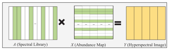
Figure 1.
Illustration of the hyperspectral sparse unmixing problem, Y is the image to be unmixed, A is the large-scale spectral library, and X is the obtained abundance matrix. Only colored active endmembers participate in the reconstruction of endmembers.
However, the SUnSAL [8] only focuses on the spectral information without taking the spatial structure information between different pixels into account. In general, a hyperspectral image () with pixels structured in the matrix can be formulated as
where , is the -th mixed pixel, is the abundance matrix, and is the corresponding error term. The formula (4) can be transformed into an optimization problem expressed as
where = , , is th row of . To take advantage of the relationship between pixels in the hyperspectral image, CLSUnSAL [9] assumes that all pixels share the same active endmembers to reduce the influence of the spectral coherence between endmembers on the unmixing effect. The model is shown as follows
where represents the norm, denotes the indicator function. Moreover, many spectral regularization terms, such as the total variation regularization term [10] and the non-local regularization terms [11], are integrated into the sparse unmixing model to promote the spatial correlation.
2.2. Multiobjective Optimization
The multiobjective evolutionary algorithms (MOEAs) have attracted extensive attention because of the global search ability in solving the sparse unmixing problems. In [15], Gong et al. proposed the multiobjective sparse unmixing model with a cooperative coevolutionary strategy. Jiang et al. [16] formulated the sparse unmixing problem into a two-phase multiobjective problem to estimate the endmembers and determine the abundances, respectively. In [17,18], the multiobjective evolutionary algorithm based on decomposition (MOEA/D) [20] has also been explored and applied in the sparse unmixing problem. For the multiobjective optimization problem, the mathematical form with a objectives and b decision variables can be described as
where is the decision vector, F: , is the decision space and is the objective space.
In the majority of cases, there is no single solution capable of minimizing all the objectives at the same time. Instead, the best trade-off between the objectives can be defined as Pareto optimality. Therefore, in order to evaluate the pros and cons of multiple solutions, the nondominated fronts and crowding distances of the individual can be applied. If the individuals are dominated by the same number of individuals, these individuals belong to the same nondominated front. In addition, the crowding distance of an individual can be obtained by calculating the side length of the rectangle formed between two adjacent individuals that belong to the same nondominated front with the individual. Assuming that and are two individuals in the population, individual is preferred over (i.e., ) if any one of the following conditions holds [21], (1) , (2) and , where and represent the nondominated fronts of individuals and , respectively. and represent the crowding distances of individuals and , respectively.
3. Proposed Method
For the sparse unmixing problem, there are two conflicting objectives to be optimized, namely the sparse endmember term and the reconstruction error term. Therefore, the multiobjective optimization problem for sparse unmixing is
where the is the sparse term and the represents the reconstruction error. The Formula (8) can be solved with the multiobjective optimization to obtain the Pareto Front (PF) of a compromise between these two objectives. Then the knee point is selected as the final solution, which is the preferred solution on PF with the maximum marginal utility and can be obtained from the individual with the maximum angle with the two adjacent individuals. In addition, two constrains for the abundance are required by
The pseudocode of the proposed EMSU-EP is shown in Algorithm 1. First of all, in the initialization, the k-th endmember is extracted from the spectral library at a time to reconstruct the hyperspectral image for obtaining the corresponding reconstruction error with the original image. This operation needs to run through all the endmembers in the spectral library. The reconstruction errors of all endmembers are sorted in ascending order, and the corresponding represents the position order. Then the spectral library is encoded into a binary vector with dimension , where “1” and “0” represent the selected and unselected endmembers, respectively. Then EMSU-EP randomly selects two elements from the D-dimensional decision variables each time, and uses the endmember score as the evaluation criterion to set one of to “1” with the binary tournament selection method, which is shown in Figure 2. In order to ensure the diversity of the initial population, the operator is employed to uniformly distribute individuals in the sparse interval [0, D], respectively. Unlike the inefficiency of random initialization, the more likely real endmembers can be selected to form the initial population with the prior knowledge.
| Algorithm 1 Pseudocode of EMSU-EP |
| Input: A (the spectral library), Y (the hyperspectral image), (population size), (maximum number of iterations). Output: (the estimated abundance map).
|
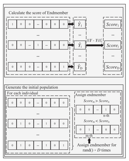
Figure 2.
Obtaining the score of every endmember and generate the initial population.
With the prior knowledge of decision variables, those decision variables with higher scores should be given more attention in the subsequent genetic operations. Therefore, the genetic operators of crossover and mutation proposed in [22] are employed to generate the offspring, which are represented by Crossover() and Mutation(), respectively, in Algorithm 1. The left gray box and the the right gray box represent the Crossover() operator and the Mutation() operator, respectively, in Figure 3. Before evolution, two individuals and are randomly selected from population as the parents. There are two situations in the Crossover(). On the one hand, the original offspring inherits , then two non-zero elements are randomly selected from the differential gene positions of and , and one of the gene positions of is set to “0” based on endmember scores (the larger the better). On the other hand, two zero elements are randomly selected from the differential gene positions of and , and one of the gene positions of is set to “1” based on endmember scores (the smaller the better). In the Mutation(), two non-zero elements are randomly selected from the offspring , and one of the gene positions is set to “0” determined by the larger score. To the opposite, two zero elements are randomly selected from , and set one of the gene positions is set to “1” determined by the smaller score. A zero or non-zero element in the binary vector is flipped with the same probability as shown in Figure 3. Compared with the single-point crossover (SPC) and bitwise mutation (BitM), the operators designed by the EMSU-EP select the element to be flipped according to the score of the decision variable to ensure the sparsity of the offspring.
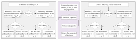
Figure 3.
Illustration of the flow of crossover and mutation operators. The middle procedure represents the generation process of a offspring, the left procedure represents the crossover operation, and the right procedure represents the mutation operation.
During the evolution of the population, if too many endmembers are selected, some solutions are no longer sparse. To prevent this problem from happening, the sparsity limit is applied to the population evolution. When the number of selected endmembers in an individual exceeds the sparsity limit , EMSU-EP will only retain the endmember whose endmember score sorting in the first -th, and the rest will not be selected (i.e., set to 0).
Finally, all individuals of the parent and offspring are evaluated for nondominated sorting and crowding distance calculation [23], and the best individuals are selected to form the next generation population. After satisfying the end of the iteration, the knee point in the last generation population is returned [24]. The set of non-zero elements are extracted from this optimal binary vector, which also represents the corresponding endmember subset from the spectral library A. Therefore, the abundance map can be calculated according to the least square method, which is shown as follows
According to the Formula (10), we can not only achieve dimensionality reduction of hyperspectral data, but also ensure the sparseness of unmixing solutions. After the calculation of Formula (10), the zero element is inserted into the non-zero real solution according to the original position to realize the restoration of the data dimension.
4. Experimental Results and Discussion
In this section, the effectiveness of EMSU-EP in solving large-scale sparse unmixing problems will be demonstrated. Two large-scale sparse unmixing benchmark datasets are used to validate the performance of the EMSU-EP. In order to reflect the efficiency of EMSU-EP, some advanced algorithms such as SUnSAL [8], CLSUnSAL [9], MOSU [15] and MTSR [21] will be compared with EMSU-EP.
In the experiment, the population size is set to 100, and the maximum generation Maxgen is set to 300, the population sparse limit interval is 50. Part of the experiment code refers to the PlatEMO platform (PlatEMO 2.8: https://github.com/BIMK/PlatEMO (accessed on 22 August 2021)) [25]. All experiments will be added with different degrees of Gaussian white noise (SNR = 20, 30 and 40 dB). All experimental results are obtained from the average of 100 independent repeated runs.
4.1. Dataset and Evaluation Indicators
4.1.1. Dataset
Data 1 is a 64 × 64 synthetic image containing 224 bands provided by Tang [26], its digital spectral library A1 is a sub-library of 498 spectral features selected from the USGS spectral library (http://speclab.cr.usgs.gov/spectral.lib06 (accessed on 22 August 2021)). These spectral signals are evenly distributed at 0.25–0.4 m. The true abundance map of all five endmembers of data 1 is shown in Figure 4. Data 2 is an image of 100 × 100 pixels and 224 bands per pixel, provided by Iordache et al. [10], its digital spectral library A2 is a sublibrary with 230 spectral signatures of the USGS spectral library. The true abundance map of all nine endmembers of data 2 is shown in Figure 5.
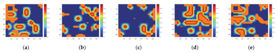
Figure 4.
True abundance maps of five endmembers in data 1. (a) True abundance map of endmember 1. (b) True abundance map of endmember 2. (c) True abundance map of endmember 3. (d) True abundance map of endmember 4. (e) True abundance map of endmember 5.
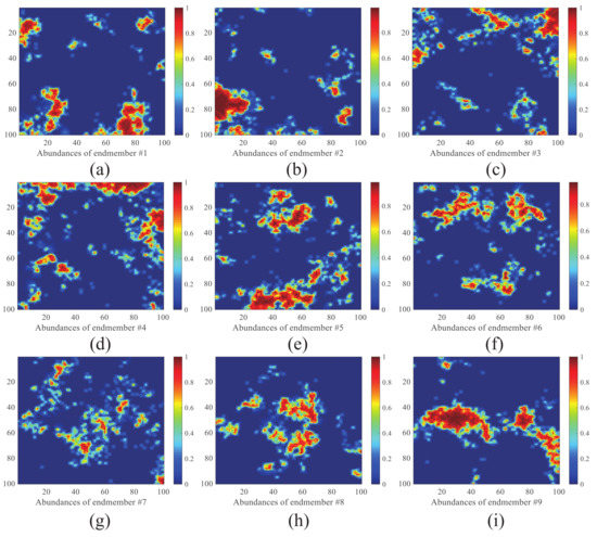
Figure 5.
True abundance maps of five endmembers in data 2. (a) True abundance map of endmember 1. (b) True abundance map of endmember 2. (c) True abundance map of endmember 3. (d) True abundance map of endmember 4. (e) True abundance map of endmember 5. (f) True abundance map of endmember 6. (g) True abundance map of endmember 7. (h) True abundance map of endmember 8. (i) True abundance map of endmember 9.
To summarize, data 1 needs to accurately select five endmembers from 498 spectral signals and estimate the corresponding abundance, and data 2 needs to select nine endmembers from 230 spectral signals and estimate the corresponding abundance. Two datasets are sparse enough and difficult. Therefore, both data 1 and data 2 are large-scale sparse unmixing problems.
4.1.2. Evaluation Indicators
In order to compare the accuracy and the robustness of different sparse unmixing algorithms on large-scale hyperspectral sparse unmixing problem, two evaluation indicators are considered in the experiments.
(1) Signal-to-Reconstruction Error (SRE) can be expressed as:
where is the true fractional abundance matrix and is the estimated fractional abundance matrix. Without loss of generality, the larger the SRE value is, the better the unmixing accuracy will be.
(2) Success Ratio (SR): If the relative error is smaller than a given threshold , the corresponding run of this method is denoted as a successful run [27]. SR under the threshold is defined as:
The probability is the ratio of the successful runs on 100 random instances. If we set = 5 and arrive at = 1, this implies that the relative error of the reconstruction result is less than 5 with probability one.
The Hypervolume (HV) [28] indicator can be used to evaluate the quality of PF, which can reflect the convergence and diversity of the solutions. HV is calculated by utilizing a reference point who is 1% larger in every component than the corresponding nadir point. In this paper, we use it to evaluate the performance on large-scale sparse unmixing problem by crossover and mutation operations of EMSU-EP, traditional SPC and BitM.
4.2. Experiments on Synthetic Data
Figure 6 shows the PF of the 50-th generation population obtained by different methods on data 1 and data 2. Whether compared to the PF obtained by SPC and BitM with the initial population of EMSU-EP or the PF obtained by SPC and BitM with the random initial population, EMSU-EP obviously has better convergence and a clearer knee point area, which will be very helpful to choose the final solution later.
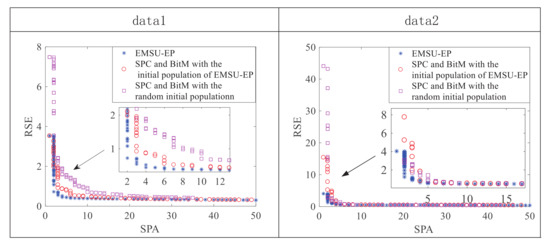
Figure 6.
Illustration of the Pareto Front of the 50th generation on data 1 and data 2.
In order to reflect the advantages of EMSU-EP in each generation, Figure 7 uses the HV indicator to evaluate the PF of the first 100 generations. As shown by the red and purple curves in Figure 7, since the SPC and BitM operation has the same initial population of EMSU-EP, a higher HV value can be obtained from the first generation compared to the SPC and BitM with the random initial population, which corresponds to a better initial population quality and shows the guiding effect of endmember scores on the production of initial population. However, as shown by the blue and red curves in Figure 7, after the 20-th generation on data 1 and the 50-th generation on data 2, there are large static difference between the HV value of EMSU-EP and the HV value of the SPC and BitM operation, which shows the guiding effect of endmember scores on the evolution of the population.
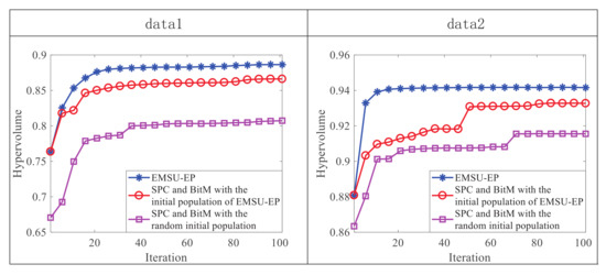
Figure 7.
Illustration of the HV value of each evolution step on data 1 and data 2.
The estimated abundance maps of some endmembers obtained by different algorithms on data 1 and data 2 are shown in Figure 8 and Figure 9, respectively. These experimental results are all on the 30dB SNR. In Figure 8, the abundance maps obtained by SUnSAL, CLSUnSAL, MOSU, MTSR and EMSU-EP are exhibited from left to right, endmember 1, endmember 2 and endmember 5 of data 1 are arranged from top to bottom. In Figure 9, the abundance maps obtained by SUnSAL, CLSUnSAL, MOSU, MTSR, and EMSU-EP are exhibited from left to right, endmember 1, endmember 5 and endmember 8 of data 2 are arranged from top to bottom. As shown in Figure 8 and Figure 9, it is obvious to see that EMSU-EP always has the best performance compared to other algorithms, the unmixing maps color of EMSU-EP is the closest to the real image. Nevertheless, the performance of EMSU-EP in reducing noise is not stable enough, only the abundance map of endmember 1 has the least noise points in Figure 8, and only the abundance map of endmember 8 has the least noise points in Figure 9. Table 1 and Table 2 show the and of the unmixing results obtained by different algorithms on data1 and data 2, respectively. The two data sets are corrupted by different levels of correlated noise (SNR = 20, 30 and 40 dB). According to Table 1 and Table 2, EMSU-EP has the highest and compared to other algorithms at three SNR levels, which indicates that EMSU-EP has the best unmixing accuracy and robustness. The experimental results of two hyperspectral datasets demonstrate that the proposed EMSU-EP method can improve the performance of the sparse unmixing model by utilizing the endmember prior information.
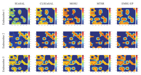
Figure 8.
The estimated abundance maps of endmember 1, endmember 2 and endmember 5 for data 1 on 30 dB SNR obtained by different algorithms.
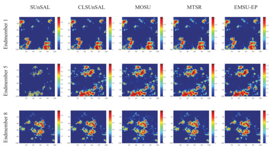
Figure 9.
The estimated abundance maps of endmember 1, endmember 5 and endmember 8 for data 2 on 30 dB SNR obtained by different algorithms.

Table 1.
Comparison of EMSU-EP with other algorithms on data 1. The value of is set to 0.15.
Table 2.
Comparison of EMSU-EP with other algorithms on data 2. The value of is set to 0.15.
5. Conclusions
In this paper, we proposed an evolutionary multiobjective hyperspectral sparse unmixing algorithm with an endmember a priori strategy (EMSU-EP) to solve the large-scale hyperspectral sparse unmixing problem. EMSU-EP reconstructs the hyperspectral image by a single endmember to generate every endmember score first. Then the obtained endmember scores are used as prior knowledge to guide the generation of initial populations and new individuals. Experiments have demonstrated that the proposed EMSU-EP algorithm is effective in solving large-scale sparse unmixing problems, and EMSU-EP can maintain the superiority compared with the state-of-the-art sparse unmixing algorithms.
In the future, we will focus on reducing the noise on hyperspectral sparse unmixing problems and exploring the further improvement of EMSU-EP performance.
Author Contributions
Conceptualization, Z.W. and J.W.; methodology, Z.W.; validation, Z.W., J.W. and F.X.; investigation, J.L.; writing—original draft preparation, Z.W., J.W. and J.L.; writing—review and editing, F.X., J.L. and P.L. All authors have read and agreed to the published version of the manuscript.
Funding
This work was supported by the National Natural Science Foundation of Shaanxi Province (grant no. 2021JQ-210), the Fundamental Research Funds for the Central Universities (Grant no. XJS200216), Key R & D programs of Shaanxi Province (Grant no. 2021ZDLGY02-06) and the National Natural Science Foundation of China (Grant no. 61973249).
Data Availability Statement
The data 1 and data 2 can be downloaded from http://levir.buaa.edu.cn/Code.htm (accessed on 22 August 2021).
Conflicts of Interest
The authors declare no conflict of interest.
References
- Shi, C.; Wang, L. Linear spatial spectral mixture model. IEEE Trans. Geosci. Remote Sens. 2016, 54, 3599–3611. [Google Scholar] [CrossRef]
- Nascimento, J.M.P.; Dias, J.M.B. Vertex component analysis: A fast algorithm to unmix hyperspectral data. IEEE Trans. Geosci. Remote Sens. 2005, 43, 898–910. [Google Scholar] [CrossRef] [Green Version]
- Miao, L.; Qi, H. Endmember extraction from highly mixed data using minimum volume constrained nonnegative matrix factorization. IEEE Trans. Geosci. Remote Sens. 2007, 45, 765–777. [Google Scholar] [CrossRef]
- Zhou, G.; Xie, S.; Yang, Z.; Yang, J.; He, Z. Minimum-volume-constrained nonnegative matrix factorization: Enhanced ability of learning parts. IEEE Trans. Neural Netw. 2011, 22, 1626–1637. [Google Scholar] [CrossRef]
- Li, J.; Bioucas-Dias, J.M.; Plaza, A.; Liu, L. Robust collaborative nonnegative matrix factorization for hyperspectral unmixing. IEEE Trans. Geosci. Remote Sens. 2016, 54, 6076–6090. [Google Scholar] [CrossRef] [Green Version]
- Berman, M.; Kiiveri, H.; Lagerstrom, R.; Ernst, A.; Dunne, R.; Huntington, J.F. Ice: A statistical approach to identifying endmembers in hyperspectral images. IEEE Trans. Geosci. Remote Sens. 2004, 42, 2085–2095. [Google Scholar] [CrossRef]
- Candes, E.J.; Tao, T. Decoding by linear programming. IEEE Trans. Inf. Theory 2005, 51, 4203–4215. [Google Scholar] [CrossRef] [Green Version]
- Bioucas-Dias, J.M.; Figueiredo, M.A. Alternating direction algorithms for constrained sparse regression: Application to hyperspectral unmixing. In Proceedings of the 2010 2nd Workshop on Hyperspectral Image and Signal Processing: Evolution in Remote Sensing, Reykjavik, Iceland, 14–16 June 2010; pp. 1–4. [Google Scholar]
- Iordache, M.; Bioucas-Dias, J.M.; Plaza, A. Collaborative sparse regression for hyperspectral unmixing. IEEE Trans. Geosci. Remote Sens. 2014, 52, 341–354. [Google Scholar] [CrossRef] [Green Version]
- Iordache, M.; Bioucas-Dias, J.M.; Plaza, A. Total variation spatial regularization for sparse hyperspectral unmixing. IEEE Trans. Geosci. Remote Sens. 2012, 50, 4484–4502. [Google Scholar] [CrossRef] [Green Version]
- Zhong, Y.; Feng, R.; Zhang, L. Non-local sparse unmixing for hyperspectral remote sensing imagery. IEEE J. Sel. Top. Appl. Earth Obs. Remote Sens. 2014, 7, 1889–1909. [Google Scholar] [CrossRef]
- Połap, D.; Woźniak, M. Red fox optimization algorithm. Expert Syst. Appl. 2021, 166, 114107. [Google Scholar] [CrossRef]
- Połap, D.; Woźniak, M. Polar bear optimization algorithm: Meta-heuristic with fast population movement and dynamic birth and death mechanism. Symmetry 2017, 9, 203. [Google Scholar] [CrossRef] [Green Version]
- Khishe, M.; Mosavi, M. Chimp optimization algorithm. Expert Syst. Appl. 2020, 149, 113338. [Google Scholar] [CrossRef]
- Gong, M.; Li, H.; Luo, E.; Liu, J.; Liu, J. A multiobjective cooperative coevolutionary algorithm for hyperspectral sparse unmixing. IEEE Trans. Evol. Comput. 2017, 21, 234–248. [Google Scholar] [CrossRef]
- Jiang, X.; Gong, M.; Li, H.; Zhang, M.; Li, J. A two-phase multiobjective sparse unmixing approach for hyperspectral data. IEEE Trans. Geosci. Remote Sens. 2018, 56, 508–523. [Google Scholar] [CrossRef]
- Xu, X.; Shi, Z.; Pan, B. l0-based sparse hyperspectral unmixing using spectral information and a multi-objectives formulation. ISPRS J. Photogramm. Remote Sens. 2018, 141, 46–58. [Google Scholar] [CrossRef]
- Xu, X.; Shi, Z.; Pan, B.; Li, X. A classification-based model for multi-objective hyperspectral sparse unmixing. IEEE Trans. Geosci. Remote Sens. 2019, 57, 9612–9625. [Google Scholar] [CrossRef]
- Chang, C.I.; Heinz, D.C. Constrained subpixel target detection for remotely sensed imagery. IEEE Trans. Geosci. Remote Sens. 2000, 38, 1144–1159. [Google Scholar] [CrossRef] [Green Version]
- Zhang, Q.; Li, H. MOEA/D: A multiobjective evolutionary algorithm based on decomposition. IEEE Trans. Evol. Comput. 2007, 11, 712–731. [Google Scholar] [CrossRef]
- Li, H.; Ong, Y.; Gong, M.; Wang, Z. Evolutionary multitasking sparse reconstruction: Framework and case study. IEEE Trans. Evol. Comput. 2019, 23, 733–747. [Google Scholar] [CrossRef]
- Tian, Y.; Zhang, X.; Wang, C.; Jin, Y. An evolutionary algorithm for large-scale sparse multiobjective optimization problems. IEEE Trans. Evol. Comput. 2020, 24, 380–393. [Google Scholar] [CrossRef]
- Deb, K.; Pratap, A.; Agarwal, S.; Meyarivan, T. A fast and elitist multiobjective genetic algorithm: NSGA-II. IEEE Trans. Evol. Comput. 2002, 6, 182–197. [Google Scholar] [CrossRef] [Green Version]
- Branke, J.; Deb, K.; Dierolf, H.; Osswald, M. Finding knees in multi-objective optimization. In Proceedings of the International Conference on Parallel Problem Solving from Nature, Birmingham, UK, 18–22 September 2004; Springer: Berlin, Heidelberg, 2004; pp. 722–731. [Google Scholar]
- Tian, Y.; Cheng, R.; Zhang, X.; Jin, Y. PlatEMO: A matlab platform for evolutionary multi-objective optimization [educational forum]. IEEE Comput. Intell. Mag. 2017, 12, 73–87. [Google Scholar] [CrossRef] [Green Version]
- Tang, W.; Shi, Z.; Wu, Y.; Zhang, C. Sparse unmixing of hyperspectral data using spectral a priori information. IEEE Trans. Geosci. Remote Sens. 2015, 53, 770–783. [Google Scholar] [CrossRef]
- Li, H.; Zhang, Q.; Deng, J.; Xu, Z.-B. A preference-based multiobjective evolutionary approach for sparse optimization. IEEE Trans. Neural Networks Learn. Syst. 2018, 29, 1716–1731. [Google Scholar] [CrossRef] [PubMed]
- Beume, N.; Naujoks, B.; Emmerich, M. SMS-EMOA: Multiobjective selection based on dominated hypervolume. Eur. J. Oper. Res. 2007, 181, 1653–1669. [Google Scholar] [CrossRef]
Publisher’s Note: MDPI stays neutral with regard to jurisdictional claims in published maps and institutional affiliations. |
© 2021 by the authors. Licensee MDPI, Basel, Switzerland. This article is an open access article distributed under the terms and conditions of the Creative Commons Attribution (CC BY) license (https://creativecommons.org/licenses/by/4.0/).