Data Transformation Schemes for CNN-Based Network Traffic Analysis: A Survey

Abstract

The enormous growth of services and data transmitted over the internet, the bloodstream of modern civilization, has caused a remarkable increase in cyber attack threats. This fact has forced the development of methods of preventing attacks. Among them, an important and constantly growing role is that of machine learning (ML) approaches. Convolutional neural networks (CNN) belong to the hottest ML techniques that have gained popularity, thanks to the rapid growth of computing power available. Thus, it is no wonder that these techniques have started to also be applied in the network traffic classification domain. This has resulted in a constant increase in the number of scientific papers describing various approaches to CNN-based traffic analysis. This paper is a survey of them, prepared with particular emphasis on a crucial but often disregarded aspect of this topic—the data transformation schemes. Their importance is a consequence of the fact that network traffic data and machine learning data have totally different structures. The former is a time series of values—consecutive bytes of the datastream. The latter, in turn, are one-, two- or even three-dimensional data samples of fixed lengths/sizes. In this paper, we introduce a taxonomy of data transformation schemes. Next, we use this categorization to describe various CNN-based analytical approaches found in the literature.

1. Introduction

1.1. Deep-Learning Approach to Network Traffic Analysis

The rapid growth of computer networks over the last decades [1] has entailed a larger amount of cyber-attacks. In order to minimize the losses, many security methods are in heavy use. Among others, network traffic analysis is in the lead. This day-to-day operation consists of processing typical patterns, such as traffic flow, bandwidth usage or resource access. Together, these patterns identify the normal network behavior, also known as a baseline. Having this baseline in mind, it is possible to interpret abnormal activities, which may indicate an attack.

Deep learning methods have also begun gaining popularity recently. This is mainly caused by the development of computing capabilities based on parallel processors originated from graphics cards. This has resulted in the rapid increase in efficient implementations of computationally demanding complex neural networks and, finally, a remarkable growth in capabilities to solve advanced problems. Among the most successful architectures of this kind are convolutional neural networks (CNNs, conv-nets). They are ideally suited for multidimensional data, originate from image processing but can be successfully applied to other computing domains.

Internet traffic analysis and machine learning are the two worlds that must be connected with one another, especially when applying the latter to the data provided by the former. The originator of the junction of traffic analysis with CNNs is Wang, who, during the innovative presentation at the “Black Hat” conference in 2015 [2], pointed out the similarities between images and TCP flow payloads. Despite the utilization of an autoencoder to identify network traffic, in a later work, Wang signaled the usefulness of CNNs for the same task. To the best of our knowledge, this is the first mention of network traffic identification or malware detection with the advantage of CNNs.

There is a striking change in the number of research papers that are devoted to the analysis of network traffic by CNN models (see Figure 1). To enhance the analysis, we distinguish three possible subjects of the articles: malware detection, traffic classification, and the junction of both. These categories are connected with datasets studied in each paper. The typical indicators of the datasets are the motifs of data, e.g., captured botnets are the foundation of the CTU-13 dataset, so each article utilizing it will belong to the malware detection group.

What is particularly interesting seems to be the overview from the perspective of traffic transformation methods before being given as an entry to the CNNs. Deep learning models require particular data formats that are rarely similar to original computer traffic. In most of the reviewed articles, the traffic data are transformed into the forms needed for the analytical part of the whole workflow. These transformations usually require performing one or more typical actions, e.g., the selection of specific network layers, trimming the data stream, or computing some traffic features. Due to the given architecture of some learning algorithms, these data transformations often demand an increase in the dimensionalities of the traffic data. The network traffic data are a time series, while the CNNs require multidimensional input consisting of equal-length samples. Due to this fact, the original traffic data must always be transformed into a format acceptable by the deep-learning models.

1.2. Our Contributions to the Topic

This survey deals with transformations of the network traffic, which are the input of the deep learning models, with particular attention paid to the CNN models. We have studied many articles and finally chose 136 papers written recently in this field of science. It is essential to highlight that other surveys present these studies from the perspective of cyber-attacks, particular system traffic, or mixed deep-learning models.

We explicitly focus on the network traffic transformations before being given as an entry to the CNN models.

• This paper proposes the new taxonomy of the network traffic transformations for CNN processing purposes.
• Additionally, all 136 revised articles are comprehensively investigated and mapped to the adequate transformation algorithms. The survey differentiates three categories of research papers:

  (a)

  Traffic classification.

  (b)

  Malware detection.

  (c)

  The combination of traffic classification and malware detection.

  The first contains all articles that focus on encrypted traffic identification. The malware detection category is about finding unwanted traffic. The last includes research about both mentioned categories. These categories are firmly connected with the datasets utilized by each group of authors. Moreover, it is possible to distinguish different themes of the datasets, such as dealing with VPN traffic or exploring features of botnets.
• This work highlights and describes the utilized datasets and the architecture of each CNN model.

The proposed taxonomy is the first on this topic. While preparing this work, we inherited and developed the concept from the CNN chapter from [3].

As the number of papers in the described field is constantly growing, we decided to review the proposed works and highlight all scientific observations. The detailed comparison in this area can establish current trends as well as enhance network traffic analysis.

1.3. Paper Structure

This paper consists of nine sections. Section 2 touches upon fundamental issues in the discussed scientific field. The following subsections are devoted to main categories of methods that reflect the ways that the network traffic is transformed prior to transferring them into the CNN-based neural models. Section 3 presents approaches based on raw traffic, i.e., network traffic without any filtering. Section 4 is about all transformations working on flows—particles of the entire traffic. Section 5 highlights data manipulations on payloads extracted from the raw traffic. Section 6 focuses on all concepts based on payload that is extracted from flows. Traffic features approaches are the main subject of Section 7. Section 8, in contrast to Section 7, gives a concrete overview of those articles that additionally focus on the feature extraction process. Section 9 concludes the paper.

2. Preliminaries

2.1. Network Monitoring

The internet is based on a protocol suite, which was developed by the Defense Advanced Research Projects Agency (DARPA). The idea of a distributed topology, with a packet switched network is described from the time perspective by its author Baran in [4]. With the rapid growth of the internet at the end of the 20th century, there was also a necessity for network accounting and monitoring. Almost in parallel to network traffic profiling for accounting reasons, frequent and large-scale network attacks have led to an increased need for developing techniques for analyzing network traffic. In the design philosophy of the DARPA internet protocols [5], Clark explained flow as being connected with the necessity to treat differently those packets transmitted by intermediary network devices with an appropriate type of service demanded by the endpoints applications. In such a way, particular packets belonging to the same connection can be distinguished. According to the basic principles of packet switching networks, each datagram from a network connection can take different routes. In the beginning, the original ARPANET host-to-host protocol provided flow control based on both bytes and packets. However, later, due to efficiency reason, only the bytes number was used for acknowledgments.

Later, at the beginning of the 1990s, Mills et al. proposed internet accounting [6]. Network accounting introduced packet aggregation based on flows, using packet header information. Then, the idea was developed to use real-time traffic flow measurement (RTFM) [7]. Claffy et al. proposed a methodology for profiling traffic flows on the internet for communication analysis [8].

Then, with the implementation of the NetFlow [9] protocol, the traditional understanding of IP flow was defined as a set of five, up to seven, IP packet attributes flowing in a single direction. When a TCP session is considered, a flow consists of all packets transmitted until this session terminates. NetFlow, among others, uses the following IP packet attributes: IP source address, IP destination address, source port, destination port, layer 3 protocol type, type of service, router or switch interface. All packets with the same earlier-mentioned attributes are grouped into a flow, and then packets and bytes are counted. With the introduction of the IP flow information export (IPFIX) protocol, the number of flow attributes, named IPFIX information elements, increased to several hundred. The RFC7011 explains that [10]: “(…) A Flow is defined as a set of packets or frames passing an Observation Point in the network during a certain time interval. All packets belonging to a particular Flow have a set of common properties. Each property is defined as the result of applying a function to the values of:

• One or more packet header fields (e.g., destination IP address), transport header fields (e.g., destination port number), or application header fields (e.g., RTP header fields [RFC3550]);
• One or more characteristics of the packet itself (e.g., number of MPLS labels);
• One or more of the fields derived from Packet Treatment (e.g., next-hop IP address, the output interface) (…)”.

In the studied papers, we have found different usages of the flow term with several nouns, such as traffic, packet, data, and IP packets, which can mislead the readers. Therefore, we have decided to unify network traffic terms for this survey as the following definitions:

• Raw traffic —network traffic observed in an observation point, such as a line, to which the probe is attached, an Ethernet-based LAN, or the ports of a switch or router [10].
• Flow (also called traffic flow (e.g., [10]), network connection (e.g., [11]), internet stream (e.g., [12]))—grouped raw network traffic according the same properties, usually 5-tuple: source and destination IP address, source and destination port number, and type of service.
• Session—bi-directional flow. Traffic grouped according to the same properties as a flow, which mimics conversation between the end devices. A session usually requires establishing a TCP connection in the form of a three-way handshake.
• Traffic features [13] (also called flow features)—set of features describing the traffic. They can be statistical features of flow data obtained from flow probe, using one of the flow profiling protocols, e.g., IPFIX, or processed using the appropriate software or particular network protocols headers fields [14]. When collected and exported in IPFIX flow records, they are called information elements (IEs) [10]. Some of these features can be exported in IPFIX flow records, using a textual representation of IPFIX [15]. A standard list of IEs is maintained by the internet assigned numbers authority (IANA). Moreover, the internet community can define their new elements, which fulfill the applications’ specifications [16]. Hofstede et al. prepared a more detailed specification of flow monitoring with NetFlow and IPFIX [17].
• Payload—transmitted data encapsulated in the particular ISO/OSI model protocol data unit (PDU). The Layer 4 (and above layers) payload (L4+ payload) are the actual upper—layers (L5, L6, L7) data, e.g., HTTP request or response—FTP data. The Layer 3 payload is a segment (TCP) or a datagram (UDP) of the Layer 4 PDU, including the L5-L7 PDUs. The Layer 2 payload (L2 payload) is a packet—usually an IP packet.

Traffic data can be collected from an observation point with a hardware or software solution. Written in C, an open-source library Libpcap (see: https://www.tcpdump.org/, accessed on: 2 July 2021) is available for different platforms. This library delivers an application programming interface (API), which can be implemented in capturing software, e.g., tcpdump or Wireshark. Collected traffic data with the libpcap library can be saved in the pcap file format and used to create a dataset for analytics and classification.

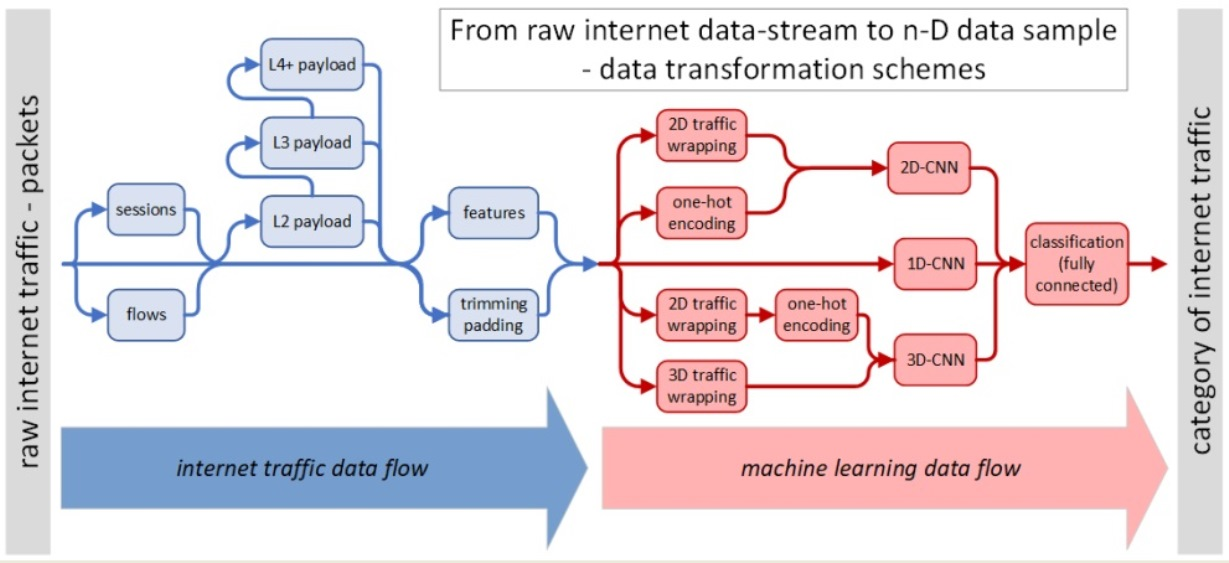
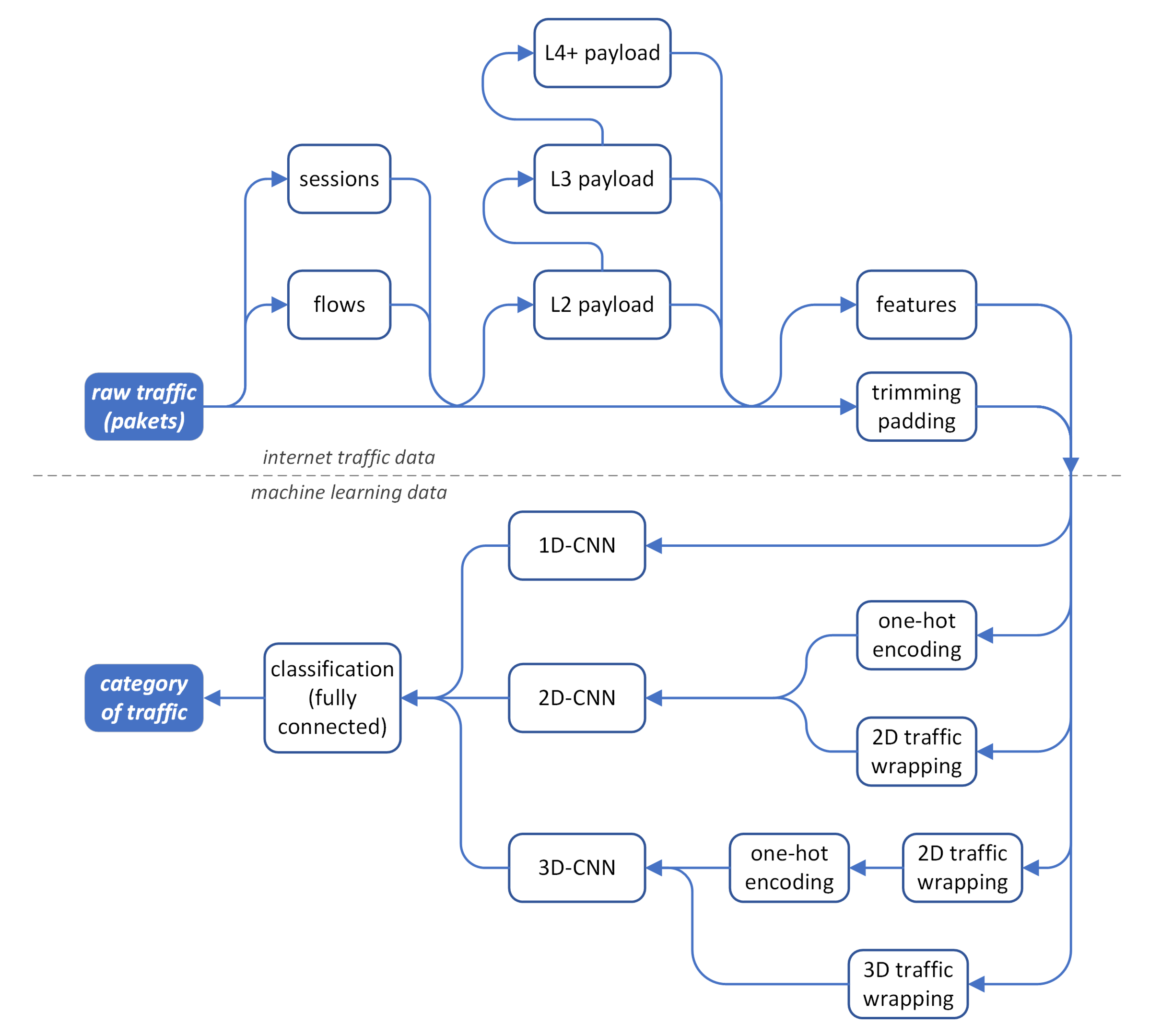
Depending on the available datasets (see Section 2.4) and implemented machine learning algorithms, traffic datasets can directly feed the chosen CNN-based deep learning model (CDM) or may have to be pre-processed according to several paths, as is presented in the upper part of the workflow diagram in Figure 2. Different possible side paths—raw traffic processing or filtering—are indicated with blue arcs.

The straightforward path is with only trimming or padding block. In the case of using only internet raw traffic for a machine (deep) learning (straight line in Figure 2), there is a necessity to change the length of the original stream data into chunks to prepare these according to the input size of the chosen CDM. If the input dimension of the selected model is smaller than the stream data chunk, the latter has to be trimmed to the size of the CDM’s input vector dimension. When the input stream is shorter than is expected by the CDM, the remaining part of the input vector is padded with an arbitrarily selected value—usually with zeros, to fit the suitable CDM’s input vector dimension.

Following two side paths—alternatively: flows or sessions—requires grouping traffic data according to the same properties. Then, the flows or sessions’ data must be trimmed or padded, again as in raw traffic, to fit the suitable CDM’s input vector dimension.

An alternate path for flows or sessions data can lead through selected layers (L2, L3, L4+) payload extraction. In intrusion detection systems (IDS), such processing is called deep packet inspection (DPI). Then again, extracted payloads must be trimmed or padded to fit the suitable CDM’s input vector dimension.

Finally, the traffic data samples became an input for machine learning data described in more detail in Section 2.2.

2.2. Convolutional Neural Networks

Deep neural networks have recently become one of the hottest methodologies applied in machine learning and pattern recognition. They provide machine learning models that surpass previous approaches. Thanks to the rapid development of computing resources and common usage of relatively cheap parallel-computing platforms, previously long-lasting machine learning tasks have become available for everyone. Among the most popular types of deep networks are convolutional neural networks (CNN) [18]. They are based on convolution operators, the weight of which is a subject of learning. Due to the multidimensional nature of convolution, the CNN has gained enormous popularity in image processing and analysis. 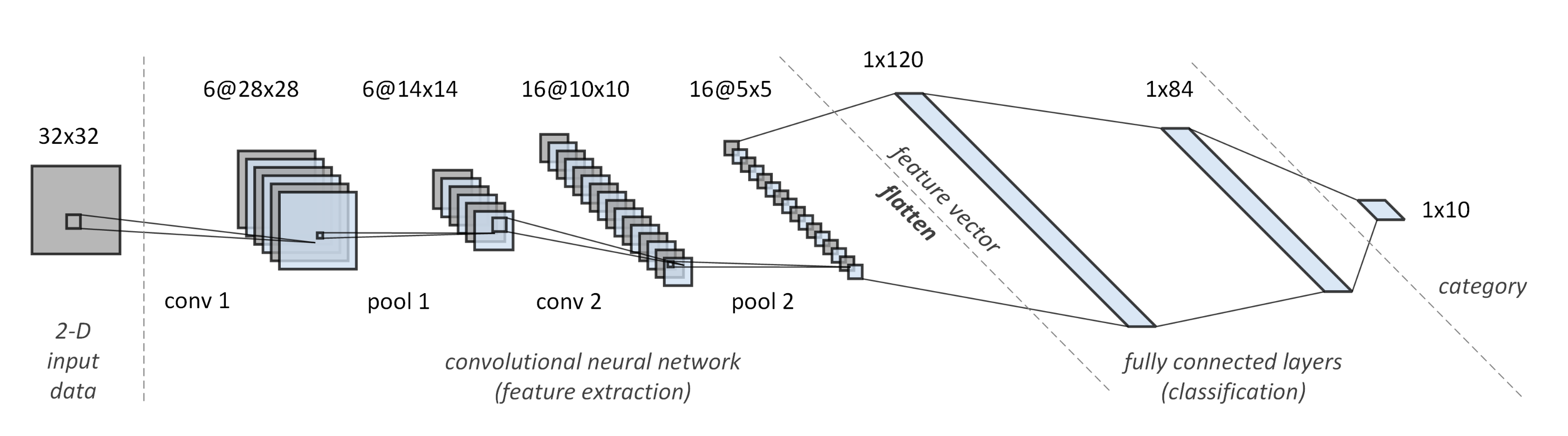Their history starts from the LeNet [19] by LeCun et al., which was a breakthrough in image pattern recognition. The CNN-based approach considerably surpassed the previous methods to classify hand-written digits recognition (MINIST datasets). It became possible because the neural network, in this case, is responsible not only for classifying the data samples (as, up to that time, typical neural nets did) but also for extracting features. In particular, the convolutional layers perform this task. In the case of conv-nets, the typical structure of the recognition scheme consists of two parts. The first one is a set of consecutive convolution layers that are stacked alternately with pooling layers. Convolution layers are responsible for extracting data features while pooling layers for reduction of the data size. The combination of feature extraction with size reduction allows for detecting data features at increasing scales. Finally, if necessary, the output of the convolution and pooling layer is flattened to obtain a final feature vector. Its further processing is a typical classification task that is usually based on the structure resembling (or sometimes being equal to) the multilayer perceptron (MLP classifier). Contrary to convolutional layers, in classification layers, all neurons located at a given layer are connected to all in the next one. Because of that, they are called fully connected (FC) or dense layers. The combination of the CNN and FC layers constitute the complete classification framework. In many papers, the name CNN is spread into the complete neural model consisting of both parts, the actual CNN and FC. However, formally speaking, it should rather be used exclusively for the first—feature extraction—part of the model. An example of such a type of network is shown in Figure 3. The diagram shows the LeNet consisting of the two parts mentioned above. The data feature extraction part inputs and the 32 × 32 image, consist of layers—convolution (conv 1), pooling (pool 1), convolution (conv 2), pooling (pool 2)—and outputs the vector of 400 data features. The classification part consists of three fully connected layers: the first with 120 neurons, the second with 84 neurons, and finally, the third with ten neurons. The number of neurons equals the number of output classes, which is equal, in this case, to the number of possible digits that might appear on the input image. For the sake of simplicity, we use shortcuts for the principal layers of the neural model: C—convolutional layer, P—pooling layer and, FC—fully connected layer. The LeNet structure may thus be coded as C|P|C|P|FC|FC|FC.

In the classic case of the image input data, the number of its dimension equals 2 for gray-level images and 3 for color ones. In the first case, it is a data array, the sizes of which equal the image sizes. In the second one, such a structure is tripled and consists of three planes of the size of an image, each of which represents one color component (in most cases red, green, and blue). The size of the third dimension equals, therefore, 3. Although the 2D and 3D above structures are mostly used in the digital image domain, the 1D input is also possible. In such a case, the convolution in at least the first layer is a 1D convolution.

Following the enormous growth in popularity of the CNN structures, they started to be applied in many domains other than vision systems. One of these domains was the categorization of the IP network traffic. In this case, the input data to be classified are samples of the network traffic. The resulting classes, in turn, are related to the types of traffic.

There are several ways of preparing the traffic data to obtain valuable input for the machine (deep) learning model described in detail in Section 2.1 (see also Figure 2). One of the possible preprocessing methods makes use of the traffic features. These features are, however, different from data features extracted by CNN. The primers are intentionally and carefully selected features of particular meaning: either properties of the traffic (e.g., IP address, port) or some statistics (e.g., number of bytes, packets). The data features, in turn, are automatically selected numbers derived from the original data vector that makes the input of the learning model.

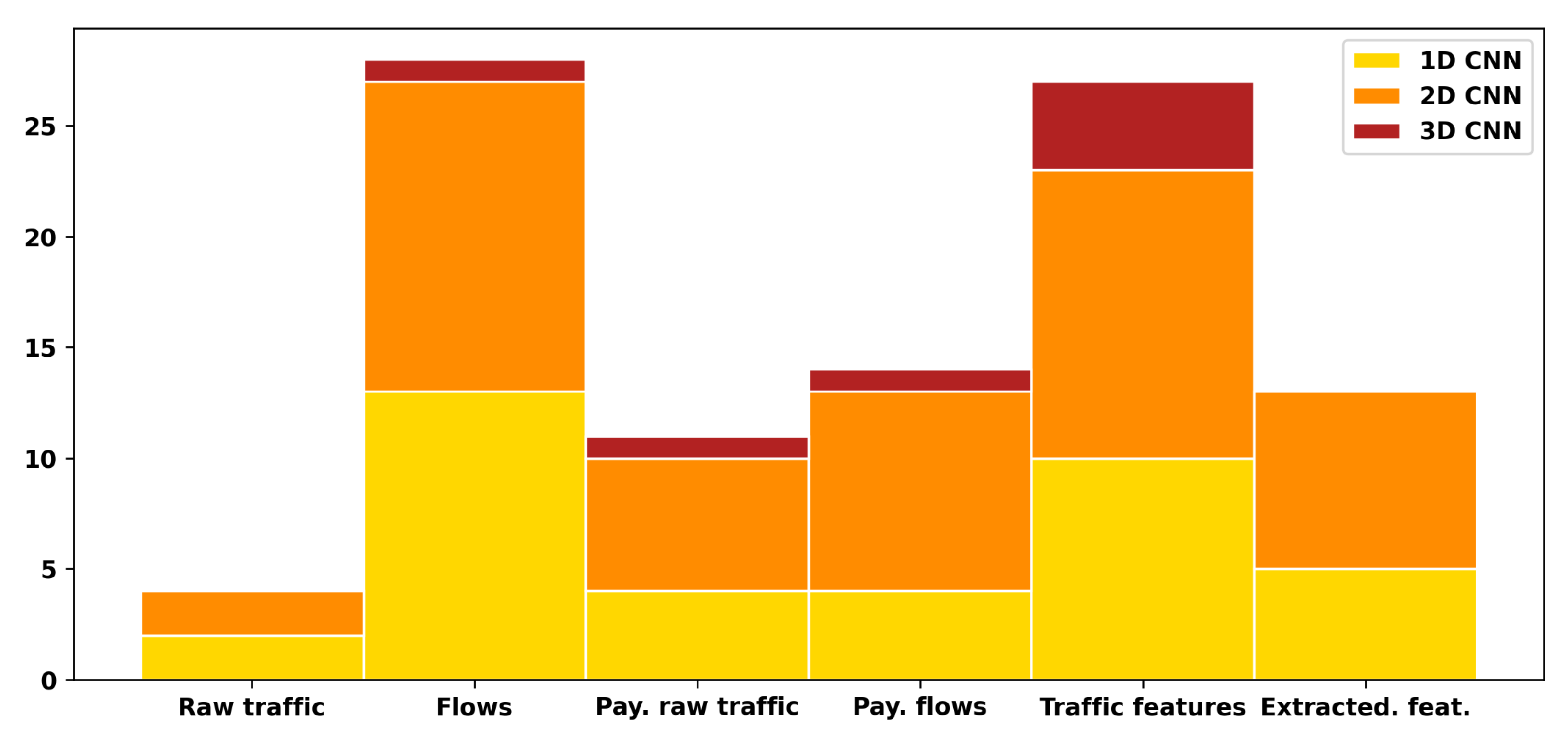
In traffic analysis applications, the input data are one-dimensional time series consisting of consecutive bytes transmitted. Following various dimensionalities of possible inputs of the CNN (1-, 2- or 3D), one may find in the traffic analysis several solutions that either keep the original 1D dimensional nature of the traffic data, or increase the number of dimensions. The 1D CNN solutions consist of 1D convolution filters, at least at the input layer. The 2D solutions add the second dimension by using, in the vast majority of cases, two approaches: traffic wrapping or one-hot encoding. The 3D solution either exploits more sophisticated wrapping or combines both techniques. The schematic diagram showing the data flow in each case is shown in the lower part of Figure 2.

Independently of the method used to add the second dimension of data, the input data for the machine learning model should consist of equal-sized data samples. To obtain such samples, data trimming (for samples originally too long) or padding (for those that are too short) is usually performed (see Section 2.1 for details).

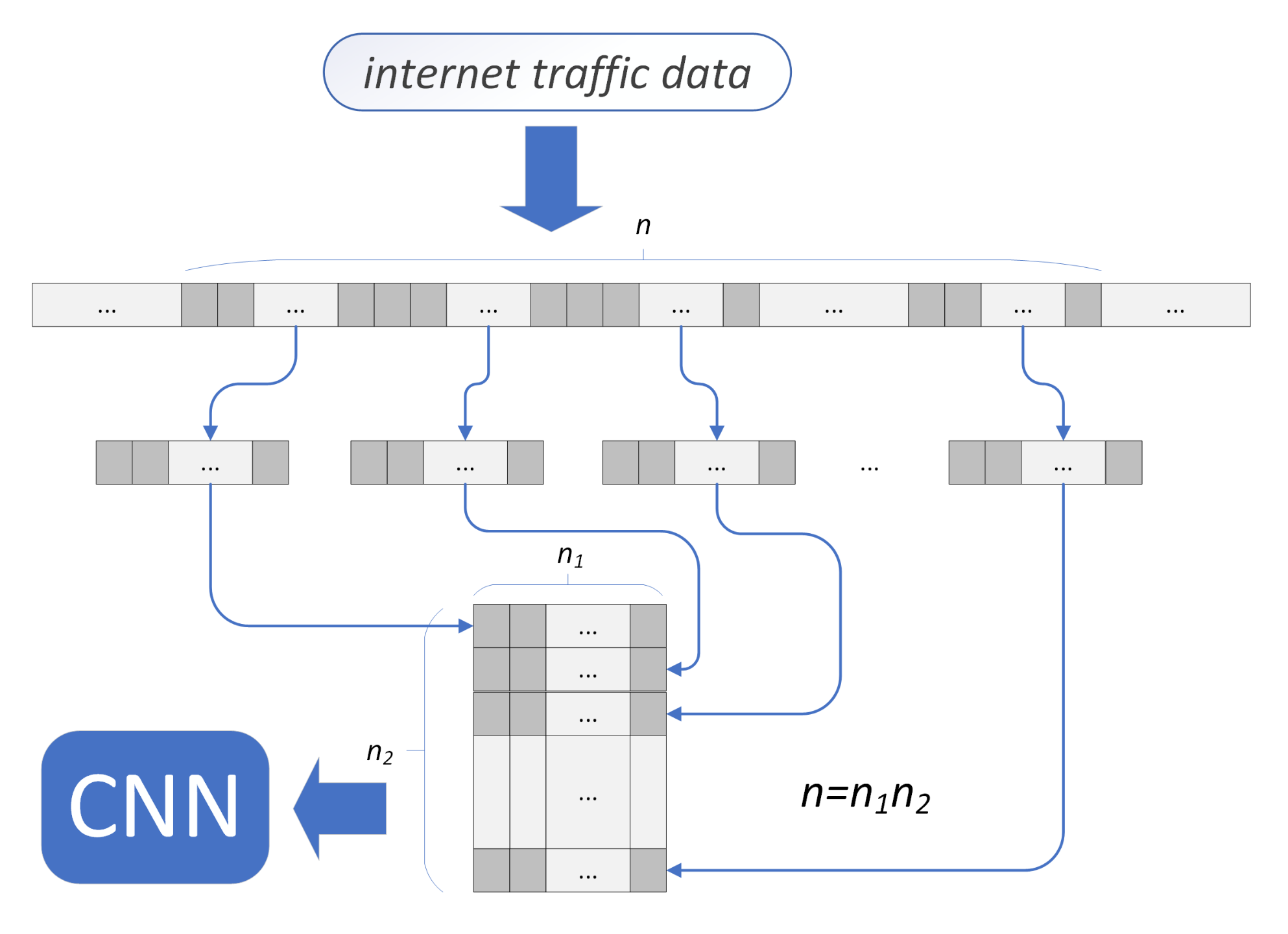
The traffic wrapping cuts the data sample consisting of n bytes into $n_2$ pieces of the same length $n_1$. Values of $n_1$ and $n_2$ are chosen in such a way that $n_1·n_2=n$. In the output data 2D array, each data value has not only neighbors that were transmitted just before and just after (these are horizontal neighbors in the 2D array), but also has vertical neighbors that, coming back to the original 1D data sample, are equivalent to the data values that appeared at a certain time before and the same time after the current data value. For example, if the data sample of size n consists of bytes, the t-th byte has two direct horizontal neighbors, $t-1$ and $t+1$, and two direct vertical ones, $t-n_1$ and $t+n_1$. The traffic wrapping is shown in Figure 4. This approach performs in a way that may be called linear stacking and is applied in all but one among the studied approaches. Several atypical approaches to 1D to 2D sample mapping (diagonal, waterfall, spirals) were studied in [20].

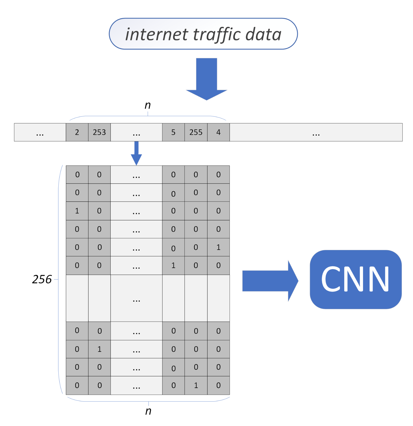
The second technique of increasing the traffic data dimensions is one-hot encoding. This approach replaces numerical integer values by the binary vector such that all but one of its elements equals zero, and the unique element equals one. Such an approach is applicable for numerical variables belonging to a finite set of m possible values (for example, a value of a byte belongs to the set of possible $m=256$ values). The one-hot-encoder thus inputs an integer of m values and outputs a binary vector of size m, containing value one at the position related to the current input values and zero elsewhere (an alternative solution encodes n-values variable as a binary vector of size $n-1$, where the n-th input value is encoded as an all-zero output). Replacing single values by vectors converts the 1D vector of integers into a 2D binary array—see Figure 5.

The origin of the one-hot encoding approach is related to the observation that—in most cases—elements of the traffic data sample (single values) are not ordered, and there is no intrinsic order of values represented by bytes. They usually represent some pieces of information encoded using bytes via standardized codes. They should thus be treated as unordered categorical values, rather than a set of consecutive integers. This property makes them different from, for example, image data, where pixel values are ordered—higher values of pixels represent a higher value of luminance. The property of having ordered values of the input data is essential in neural network learning algorithms, which are inseparable parts of the neural models that use gradient descent approaches to modify network weights iteratively.

The one-hot-encoded vector is the sparse 1D data structure of the length equal to the encoded variable’s possible values. Making it shorter is possible, using another classic trick—the embedding technique. It produces a shorter vector of a given length of possibly the same amount of information as the one-hot-encoded input. The vector embedding is performed using a fully connected layer that takes a binary one-hot-encoded vector as the input and produces a shorter embedding vector further processed by the convolution layer(s).

The architecture of the neural models consists of classic convolution, pooling and fully connected layers. It also includes often typical mechanisms found in other deep-neural models, such as regularization (mostly drop-out), preventing overfitting, or softmax output normalization that allows for interpreting the output of the model as probabilities.

In many neural approaches to network traffic analysis, pre-trained neural CNN-based models are used. They gained popularity in the image analysis domain due to their effectiveness and ability to work as backbones in many image analysis fields. In their case, the transfer learning approach in most widely used, where the image pre-trained model is learned to adapt to the network-traffic data. Pre-trained models focus on recognizing single objects located within the image and work usually on images with fixed sizes. To this group belong the following well-known networks: LeNet [19], AlexNet [21], GoogLeNet/Inception [22], DenseNet [23], ResNet [24], VGG [25], XCeption [26], and MobileNet [27].

2.3. Visual Aspects of the Traffic Data

The visualization of the network traffic is one of the classic approaches to traffic monitoring. The most traditional way is visualizing network structure as graphs where nodes and edges represent the network topology. A routing graph is a typical example of such visualization. However, this is just one of the possible network visualizations. Along with developing the internet and constantly increasing abilities to process traffic data, data visualization techniques have always played a significant role in this field. There have been many contributions in this field since the first editions of the Visualization for Cyber Security (VizSec) forum [28,29]. To perform meaningful visualizations, in some cases, authors use data reduction methods, e.g., PCA for dimensionality reduction [30].

Thanks to transforming the 1D time series of the original traffic data into 2- and 3-matrices, one may look at network traffic as digital images [31]. The single elements of the traffic data samples—which, in most cases, are simply bytes—play the role of pixels. The luminance of the pixel refers to the value of a particular element/byte, where higher byte values are represented by lighter pixels. The 1D traffic data converted into higher-dimensional data samples of a fixed length may be displayed as binary, gray level, or color images. In the first case, the input must be binary. One uses this type of traffic-to-image transformation in the case of one-hot-encoded network traffic. In the case of gray-level images, image pixels, one usually applies wrapping techniques. The resulting gray-level image looks like an image of a texture, including either irregular or regular patterns. In rarer cases, the resulting image is a color one, which is the 3D data structure. The third dimension has a fixed size of 3, due to the number of planes referring to three color components. Each of them is a gray-level image with the luminance value associated with the intensity of a particular component.

They interpret the network-traffic samples as images allowed for directly applying the image-processing techniques to this type of, initially, non-image data. They have been used, e.g., for detecting anomalies in internet traffic [32,33].

Because 2- and 3D CNN-based neural models were initially developed to process digital images, image representation of traffic has become an obvious visualization method in the CNN-based neural models. Since the ready-to-use neural backbone models are designed to process the input data of a fixed size, the size of the traffic data sample must become compliant with the input image size.

Because 2- and 3D CNN-based neural models were initially developed to process digital images, image representation of traffic became an obvious visualization method in CNN-based neural models. Since the ready-to-use neural backbone models are designed to process the input data of a fixed size, the size of the traffic data sample must become compliant with the input image size. This fact is noticeable in many network models where the size of the traffic data sample is equal to the size of the input of the neural model initially developed to process images of particular sizes. A typical example of such a strict dependence of the traffic data sample and the input of pre-trained backbone is a sample size that equals 784, which appears in many approaches. They also force the 2D input of the neural model equal to be a square array, where the length of the edge equals 28 ($28\times 28=784$)—see [34]. Such a choice is not motivated by the particular properties of the network traffic, but by the neural LeNet model, which was originally used to recognize hand-written digits on squared bitmaps of size $28\times 28$. 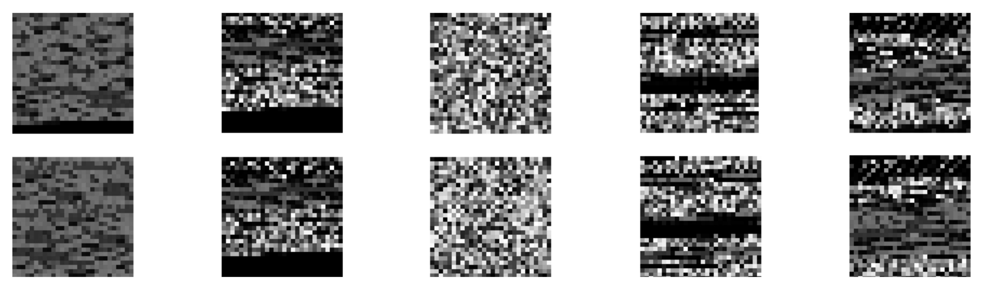Examples of images of network traffic processed using the method [34] are shown in Figure 6. The grayscale images are built from matrices using flow wrapping. The hexadecimal value of black pixels stand for 0x00, and white ones for 0xff. One may see that different samples of the same traffic (rows) look similar, while images derived from different types of internet traffic differ from one another (columns).

2.4. The Datasets

The crucial role in all machine learning methods is that of the datasets. They are necessary to perform the learning process of classifiers. They also help compare various approaches. In the case of traffic classification, several open datasets are commonly used in papers under study. The datasets include various types of traffic data: raw traffic, flows and features. Short characteristics of the most frequently employed in the studied papers are listed in

Table 1. The summary of the most popular datasets used in the studied papers—sorted by the year of creation.

Dataset	Applied in	Format	Size [GB]	Year
KDD Cup 1999	9 articles: [35,36,37,38,39,40,41,42,43]	features	0.74	1998
NSL-KDD	7 articles: [38,43,44,45,46,47,48]	features	0.04	2009
ISCX-IDS-2012	6 articles: [49,50,51,52,53,54]	flow, raw packets	8.42	2012
CTU-13	5 articles: [55,56,57,58,59]	features, raw packets	74.27	2013
UNSW-NB15	5 articles: [31,42,60,61,62]	features, flow, raw packets	0.55	2015
ISCX VPN-nonVPN	19 articles: [12,49,51,57,63,64,65,66,67,68,69,70,71,72,73,74,75,76,77]	features, raw packets	28	2016
USTC-TFC2016	11 articles: [34,66,68,69,78,79,80,81,82,83,84]	raw packets	3.71	2017
ISCX-IDS-2017	5 articles: [42,49,54,85,86]	features, flow, raw packets	51.1	2018

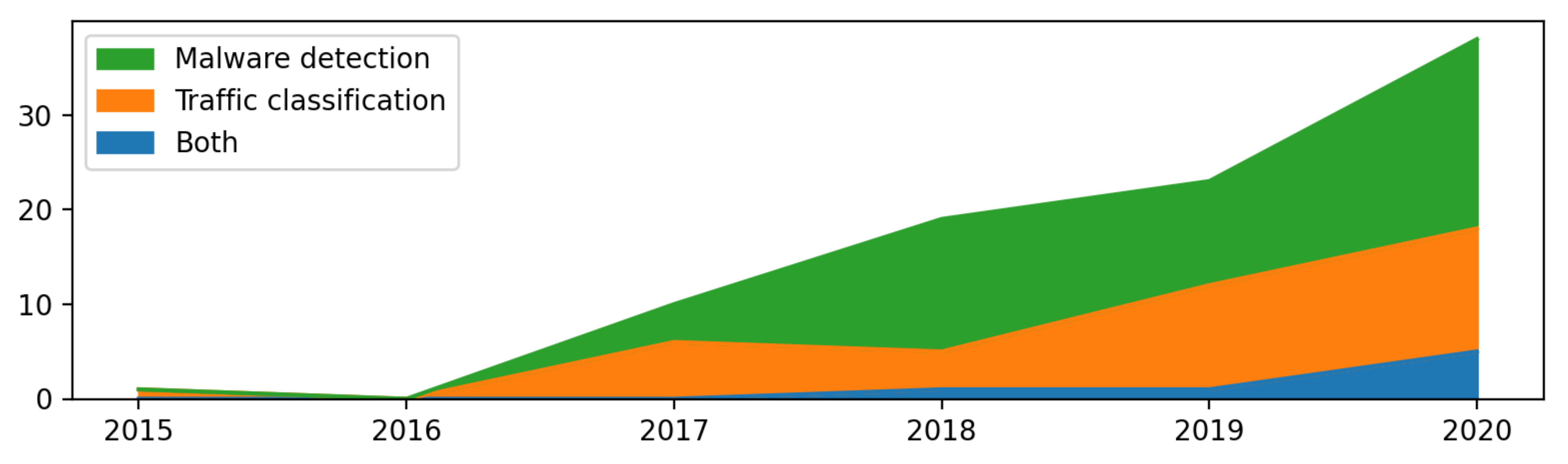
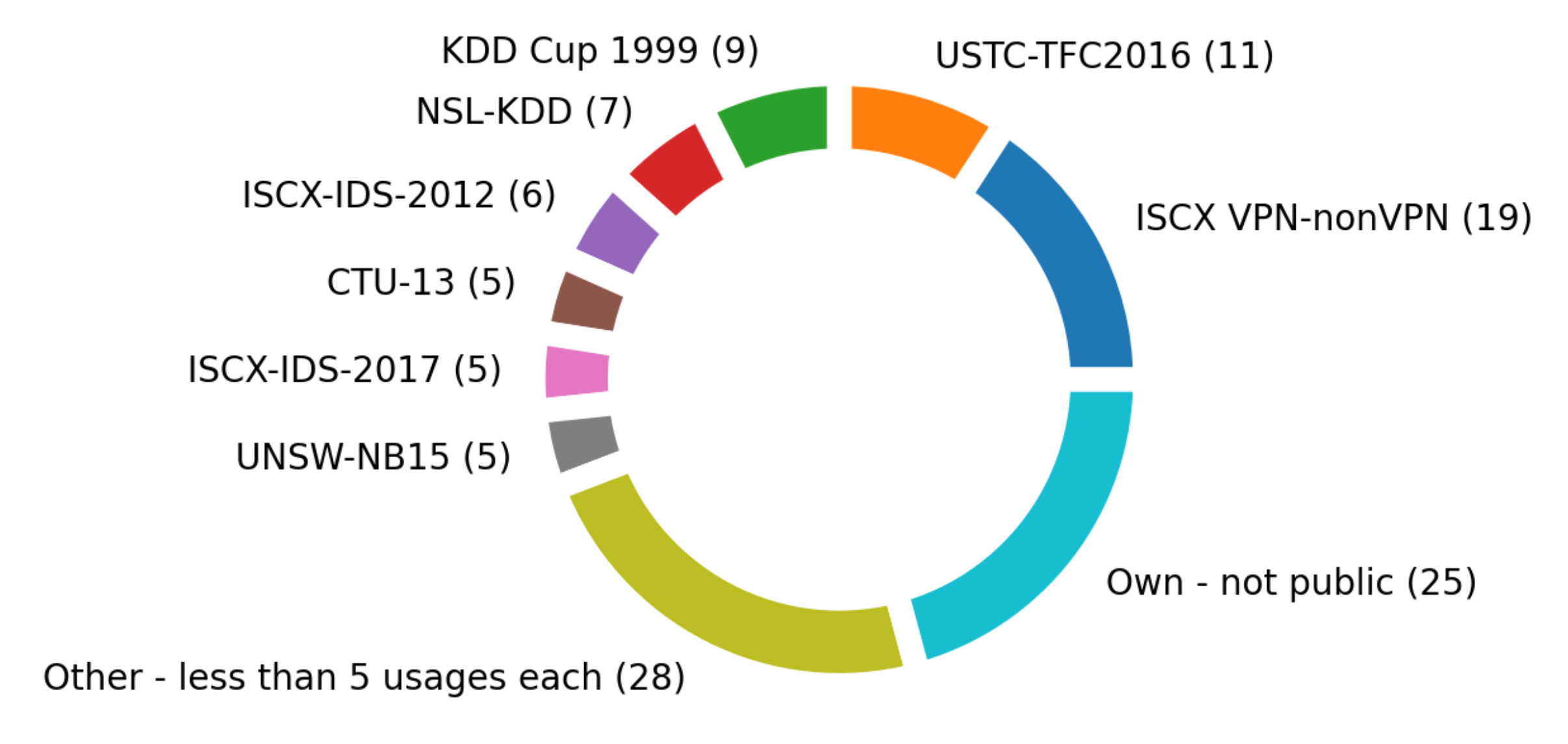
. Figure 7 shows the popularity of particular datasets in the investigated papers.

The group of 28 articles use less popular datasets (Figure 7). These datasets in alphabetic order are as follows:

BoT-IoT, CAN 2017, CIC-AAGM2017, CIRA-CIC-DoHBrw-2020, CSE-CIC-IDS2018, CTU-Malware, CTU-Mixed, DARPA 1998, DARPA 1999, EDU1, ISCX-Bot-2014, ISCX Tor-nonTor, Malware Capture Facility Project (malware), MAWILab, Mirai-RGU, NIMS, NLANR AMP, NLANR MAWI, SCU-RNE, UPC Broadband Traffic Research group’s dataset, VAST 2013 challenge and WRCCDC.

All the datasets contain a certain number of labeled traffic samples. Labels refer to the traffic classes. Classes always belong to one of two groups. In most cases, these groups are malware and benign traffic. One dataset, VPN-nonVPN, contains classes grouped according to the VPN connections within the frames of which the traffic was registered. For details regarding classes, see

Table 2. The traffic details of the most popular datasets. Datasets are sorted by the number of occurrences in articles.

Dataset	Type of Data	Traffic Details
ISCX VPN-nonVPN	encrypted	14 classes: Browsing, VPN-Browsing, Email, VPN-Email, Chat, VPN-Chat, Streaming, VPN-Streaming, File Transfer, VPN-File Transfer, VoIP, VPN-VoIP, P2P and VPN-P2P [63].
USTC-TFC2016	malware	20 classes: 10 malware and 10 benign traffic. Malware: Cridex (a worm), Geodo (a trojan), Htbot (a backdoor), Miuref (a trojan), Neris (a botnet), Nsis-ay (a botnet), Shifu (a trojan), Tinba (a trojan), Virut (a botnet), Zeus (a trojan). Benign traffic: BitTorrent, FTP, Facetime, Gmail, MySQL, Outlook, SMB, Skype, Weibo, WorldOfWarcraft [34].
KDD Cup 1999	malware	41 traffic features and 22 attacks. The 4 attack categories are: Dos, R2L, U2R and Probing [43].
CTU-13	malware	7 botnets: Neris, Rbot, Virut, Menti, Sogou, Murlo, NSIS.ay in 9 different characteristics: IRC, SPAM, ClickFraud, Port Scan, DDos, FastFlux, P2P, HTTP and compiled and controlled by the researchers [88].
ISCX-IDS-2012	malware	4 attack scenarios: Infiltrating the network from the inside, HTTP DoS, DDoS using an IRC botnet and SSH brute force [87].
NSL-KDD	malware	41 features and 1 label. The 3 groups of features are basic features, content features; and traffic features. Possible attack labels are: DoS, probe, U2R and R2L [45].
ISCX-IDS-2017	malware	16 types of attacks: Brute Force (FTP-Patator, SSH-Patator), DoS/DDoS (DoS slowloris, DoS Slowhttptest, DoS Hulk, DoS GoldenEye, DDoS LOIT), Web Attacks (Brute Force, XSS, SQL Injection), Infiltrations (Dropbox download, Cool disk – MAC), Bugs/Exploits (Heartbleed, Meta exploit Win Vista), Botnet ARES and Port Scan [89].
UNSW-NB15	malware	9 types of attacks: Fuzzers, Analysis, Backdoors, DoS, Exploits, Generic, Reconnaissance, Shellcode and Worms [90].

.

There are many datasets used in scientific papers for network monitoring and classification. They usually consist of real or simulated data. Some of them are described only in publications but are not available for other researchers for methods evaluation. In this survey, we have selected and compared only those datasets that were used in the research described in the studied papers. A comprehensive analysis that highlights datasets utilized for IDS concepts purposes is in [87]. The paper touched upon the question of pcap and NetFlow differences. It analyzed common datasets concerning the wanted traffic occurrence (not malware), the data format, anonymity, volume of the traffic, type of traffic, labeling, etc. It is crucial to point out that some described datasets are publicly available.

Having a given dataset, in the case of network traffic classification, one follows the classic machine learning workflow. The dataset is divided into training and testing sets. The former is used to train the neural model, while the latter is used to test it. However, this workflow is preceded by transforming the network traffic data into data samples that the neural model may use. Finally, the evaluation of the results is usually performed using typical measures: precision, recall, accuracy, and F1-score.

2.5. Other Surveys

Because the classification of computer network traffic seems to be a leading trend in the latest research, many surveys have been published that widely discuss this topic. However, each paper examines the scientific problem from a different perspective.

Identifying malware by machine learning techniques was widely investigated in [91]. The paper focused on different types of malware analysis. In addition, one can find a brief description of common malware types. Then, feature selection, classification, and clustering for malware detection were discussed. Finally, the authors mentioned trends of malware development. The survey did not focus on network traffic.

Another paper [92], was written on the subject of traffic classification for quality of service purposes. The article examined many machine learning methods and their advantages for anomaly and intrusion detection. It is important to highlight that the survey also discussed the practicality of the methods. Unfortunately, when it comes to CNNs, there was only one paragraph fully devoted to the history of CNNs.

Unwanted network traffic detection in the Internet of Medical Things (IoMT) was extensively discussed in [93]. Researchers analyzed types of malware attacks, architectures of the IoT environment and taxonomy of security IoT protocols. The latter focused on key management, authentication, access control and intrusion detection. The article stated that future research will be based, among others, on blockchain usage and cross-platform detection.

Work in the topic of Android malware classification was categorized in [94]. In the paper, a novel taxonomy of android malware families was introduced. The interesting part of the paper is a list of Android malware datasets and the surveyed articles’ limitations. The paper finished with future directions.

A comprehensive review of malware analysis tools that detect and analyze malware executables is given in [95]. Except for reverse engineering tools as well as memory forensics, packet analysis, detection tools, online scanners and sandboxes were elaborated.

Deep learning techniques were introduced as those that can quickly solve complex problems [96]. The article highlighted the following architectures of deep neural networks (DNNs): feed-forward neural network (FNN), convolutional neural network (CNN), recurrent neural network (RNN) and generative adversarial network (GAN). One section touched on the deep learning private data frameworks. The deep learning threats and attacks, as well as defense techniques, were also examined.

A survey [1] for collecting articles that propose deep learning-based modes to find intrusion in the network data was introduced. In the paper, one can find the taxonomy of deep learning models. In the list of research papers on supervised instance classification models for intrusion detection, there is a brief mention of [34]. The authors, among others, concluded that advances in deep learning methods are noticeable. On top of that, they said that it is often impossible to reproduce some deep learning models, due to the lack of adequate information. The authors also proposed a novel classification of four network traffic datasets.

The utilization of deep learning methods for the purposes of cybersecurity was examined in [97]. The paper singled out types of machine learning, types of deep learning and algorithms for both. Then, deep learning platforms were examined. Finally, the article outlined network attacks. CNN usage by [34] was only mentioned. The detection of cyber-attacks to the IoT infrastructure with the advantage of deep learning articles was widely discussed in [98]. The researchers reviewed the IoT architecture, reference models and IoT protocols. Then, they introduced threats against IoT systems and continued with intrusion detection systems (IDS). An interesting IDS taxonomy was also described in the paper. In the CNN section, they mentioned a few articles, but only [34] is related to security, based on network traffic. The next survey dealt with the development and detection trends of unwanted software [99]. In addition, the authors focused on those areas that were omitted by other surveys, e.g., advances in the creation of new types of malware.

The detection of intrusions throughout analysis of images generated from network traffic was outlined in [100]. The paper distinguished classical and neural networks methods. The authors dwelt on deep learning models of the convolutional neural network (CNN), long short-term memory (LSTM), support vector machine (SVM) and hybrid ones. When it comes to only CNN models, they detailed the works of [20,34,56,85]. This review points out that [101] was one of the first concepts of converting network traffic to images. The paper aroused our interest. The work proposed the creation of two-dimensional images that consist of 4 bytes in an IP address structure. The matrix then shows the intensity of traffic in the image representation. Nevertheless, this idea does not refer explicitly to CNN, and is not covered in further sections of this survey.

A systematic literature review highlighted interesting trends in the IoT infrastructure [102]. The researchers concluded that the majority of attacks take place in the network layer. There is a mention of the most popular datasets as well as common attacks.

Network traffic classification algorithms, for instance, based on the port number, statistical characteristics, host behaviors and deep learning, was considered in [3]. The last category encapsulated the following models: stack autoencoder (SAE), CNN, LSTM and deep belief networks (DBN). The CNN section described only three methods, where the CNN input was transformed beforehand—From the one-dimensional data to different one-dimensional data, to two-dimensional data or to three-dimensional data.

While preparing this survey, we decided to develop the concept of describing nothing but the CNN models’ usage for traffic classification and malware detection purposes. Contrary to [3], our article consists of 91 papers, i.e., all papers on this topic written until 2021. The conclusion of the CNN chapter in [3] is that the transformation from the 1st dimension to the 3rd dimension is better than other transformations. We believe that it is hard to hypothesize with only a few examples. On top of that, the compared examples utilized a variety of methods. Therefore, the proposed survey inherits and enhances the classification of different forms of transformations.

3. Raw Traffic

The first group of transformation methods works on the captured packets as they come in—the raw traffic. This type of data seems to be the most direct input of the CNN-based deep learning model (CDM), as its considerable merit is the lack of necessity of the prepossessing phase. However, only four research groups decided to base their work on this type of data while crafting the CNN input. These are 1D transformation [78] and 2D input concepts [35,103] (see

Table 3. The summary of articles that are in the raw traffic transformation group.

Article	Input Dimension	Layers	Dataset	Year
[78]	1D	C|P|C|P|FC|FC	USTC-TFC2016	2018
[103]	2D (200 × 200)	C|C|P|C|P|C|P|F|FC|FC|FC	EDU1	2019
[35]	2D (28 × 28)	LeNet [19]	DARPA 1999	2020
[79]	1D, 2D	C|C|P|C|C|P|F|FC|FC|FC	USTC-TFC2016	2019

). In addition, ref. [79] proposed both a 1D approach and a 2D one.

The one-dimensional entry to CNN is a vector created from raw traffic packets. While transforming packets, Marín et al. proposed the removal of only two attributes of traffic from protocol data units (PDU), i.e., MAC and IP addresses [78]. After that, a fixed size of 1300 bytes is set. It means that all longer packets are trimmed, while smaller packets are zero-padded. In the end, each packet is labeled to be either benign or malware. Finally, vectors are given to the 6-Layer CNN, which is tested on the USTC-TFC2016 dataset. This is an unwanted traffic detection approach.

The idea of wrapping raw traffic packets into the matrix was proposed by Ko et al. to test an 11-Layer CDM [103]. Traffic originated from the EDU1 dataset. This research proposed 200 × 200 bytes images. This is a traffic classification approach.

The scientific concept of raw traffic packets wrapping was further studied by Jia et al. [35]. The traffic images were based on the DARPA 1999. The authors unified the packets length so that each reached 784 bytes. Then, they wrapped the vector to create a matrix of 28 × 28 bytes size. The paper provided the images as an entry for LeNet [19]. The work’s aim was to enhance malware detection—in particular, the detection of intrusions.

The following paper, written by Zhang et al., used two different versions of CNN input [79]. The 1300 bytes size vectors are given to two 10-Layer CDM. 2D CNN obtains a traffic matrix, whose size is not revealed. It is important to highlight that vector as an entry to 1D CNN achieves better results than the matrix given to the 2D CDM. In the proposed approach, the packets are left unchanged. The deep learning model works on raw traffic from the USTC-TFC2016 dataset to detect malware. The paper proposed two types of transformations.

4. Flows

Flows, grouped raw network traffic according to the same properties, form the second part of network traffic that could be processed while preparing CNN entries. Some papers work on datasets that already consist of flows, whereas others order the raw traffic to pick up all packets belonging to each flow.

4.1. One Dimensional CNN Input

A big group of research articles processed, in CNN-based tools, vectors built from flows. The transformations are basically differentiated in two areas: sizes of input vectors and data manipulations [49,64,66,80,81,82,104,105] (

Table 4. All research works of the flow transformation method.

Article	Input Dimension	Layers	Dataset	Year
[104]	1D	C|FC|FC	MAWILab	2019
[105]	1D	same as [104]	CTU-Malware	2019
[80,81]	1D	same as [104]	USTC-TFC2016 and CTU-Malware	2019 and 2020
[64]	1D	EMB|C|C|C|C|P|FC|FC	ISCX VPN-nonVPN	2019
[82]	1D	C|P|C|P|FC|FC|FC| FC|FC|FC|FC	USTC-TFC2016 and Mirai-RGU and own	2020
[66]	1D	C|C|P|C|C|P|C|C|C| P|C|C|C|FC|FC|FC	USTC-TFC2016 and ISCX VPN-nonVPN	2020
[49]	1D	C|P|C|P|FC	ISCX VPN-nonVPN, ISCX-IDS-2012 and ISCX-IDS-2017	2020
[34]	2D (28 × 28)	C|P|C|P|FC|FC	USTC-TFC2016	2017
[55]	2D (28 × 28)	C|C	CTU-Mixed and CTU-13	2018
[56]	2D (28 × 28)	DenseNet [23]	CTU-13	2018
[106]	2D (16 × 16, 20 × 20, 28 × 28 and 32 × 32)	C|P|C|P|FC	ISCX-Bot-2014	2018
[60]	2D (28 × 28)	C|P|C|P|FC	UNSW-NB15	2018
[57]	2D (32 × 32)	C|P|C|P|C|C|FC	CTU-13 and ISCX VPN-nonVPN	2018
[50]	2D (256 × 600 and 256 × 800)	C|P|C|P|FC	DARPA 1998 and ISCX-IDS-2012	2018
[58]	2D (28 × 28)	LeNet [19]	CTU-Mixed and CTU-13	2020
[68]	2D (28 × 28)	C|P|C|P|C|P|C|P|FC	ISCX VPN-nonVPN and USTC-TFC2016	2020
[63]	1D, 2D (probably 28 × 28)	C|P|C|P|FC|FC	ISCX VPN-nonVPN	2017
[83]	1D, 2D(NS),3D	C|C|P|C|C|P|FC|FC	USTC-TFC2016	2018
[107,108]	1D, 2D (28 × 28)	same as [34,63]	Own	2018
[67]	1D, 2D (28 × 28)	same as [63]	ISCX VPN-nonVPN	2019
[65]	1D, 2D (NS)	C|P|C|P|FC	ISCX VPN-nonVPN	2020
[12]	1D, 2D (28 × 28 and other square images)	same as [34,63]	own	2020
[69]	1D, 2D (32 × 32)	C|P|C|P|C|FC	ISCX VPN-nonVPN and USTC-TFC2016	2020

).

An extended version of [78] was widely elaborated by Casas et al. for flow vectors in network security, i.e., malware detection [104]. The authors decided to use only two packets and the first 100 bytes of each. This approach was based on statistical calculations. The 3-Layer CDM was tested on the MAWILab dataset.

The same research group, Marín et al., continued to investigate malware detection [105]. The authors checked the same, previously proposed CNN tool with vectors crafted from flows of the CTU-Malware dataset. Then, the tests were extended with USTC-TFC2016 in the next two papers [80,81]. In each, the 3-Layer CNN obtained the flow vector as an input. The articles also tested different machine learning models, also not related exclusively to CNNs.

The objective of traffic classification enhancement was set out by Song et al. in [64]. The authors utilized 8-Layer CDM, which contains an embedding layer (EMB). Pcaps from ISCX VPN-nonVPN were then transformed to flow vectors to test the CNN models. Traffic prepossessing was done according to the idea of Wang Wei et al. [34]. Wang’s concept is described in the next subsection. After the normalization process, the one-hot encoding method was used for each byte in the vector, which enlarges up to 255 different values of bytes. The matrix consists of concatenated vectors. To increase the speed and effectiveness of the process, all one-hot-encoded vectors of the matrix are converted into low-dimensional dense vectors.

Hwang et al. widely tested different sizes of CNN input vectors [82]. An example of the vector is 2 by 50 bytes, which means two flows and 50 bytes of each. The researchers used pcaps from the USTC-TFC2016, the Mirai-RGU and their own datasets. The introduced 11-Layer CDM to deal with malware detection, especially anomaly detection problems.

The proposed concept of Chen et al. can determine whether traffic belongs to any of the known classes [66]. The idea requires unchanged flows that form vectors, which later become the input of the 16-Layer CDM. This function enhances the capability of the detection of yet-unknown traffic. The tool was tested on two datasets: USTC-TFC2016 and ISCX VPN-nonVPN. This article is an example of both approaches: traffic classification as well as malware detection.

Flows were also used by Chen et al. to form a 1D-CNN input [49]. Vectors of the sizes of 784 bytes were created due to the idea of [63]. Three different datasets—ISCX VPN-nonVPN, ISCX-IDS-2012 and ISCX-IDS-2017—were used to check the proposed 5-Layer CDM’s effectiveness. The CDM classifies traffic.

4.2. Two-Dimensional CNN Input

Contrary to the previously described approaches, the two-dimensional CDM input requires increasing the dimensionality of the traffic data. Flow wrapping seems to be one of the leading trends of traffic manipulations within discussed CNN entries [34,50,55,56,57,58,60,61,68,106] (Table 4). The practical concept, which started in 2017, wraps the network traffic data into the matrix [34].

The very first article that fulfilled the concept of [2] is the paper written by Wang Wei et al. [34]. This paper seems to be the first practical approach to utilize CNNs to process network traffic. Ref. [34] uses 6-Layer CNN to detect malware in the USTC-TFC2016 dataset. The authors decided to give the CDM a matrix of 28 bytes per 28 bytes. The process of creating the image (matrix) is the following: raw traffic packets are aggregated into flows or sessions, and then data are anonymized. The next step is to trim the flows to 784 bytes and ’wrap’ the vector so then one has a matrix of 28 × 28 bytes, visualized as a gray level image. The authors decided to share the tool used to create the matrix. While aggregating the packets into flow, one can choose one of the four versions of the process:

• Trim according to flows with all network layers;
• Trim according to flow with only Layer 7 (L4+);
• Trim according to session with all network layers;
• Trim according to sessions with only Layer 7 (L4+).

The choice of the only L4+ could have been placed in Section 6 of our survey. Nevertheless, the remaining two aggregating methods are also widely discussed in the paper, and this indicator makes the paper ideal for this section.

Moskalenko and Moskalenko proposed a typical flow wrapping to check 2-Layer CNN for malware detection [55]. To create the matrix, raw packets are aggregated into flows. Then, 784 bytes of sequential flows are taken to create a wrapped vector—the matrix of 28 × 28 pixels. The last step is to normalize the matrix values (pixels’ brightnesses) in the range [0,1]. The CDM is tested by pcaps from the CTU-Mixed and CTU-13 datasets.

Flow wrapping is also utilized to detect malware—more specifically, botnets by Taheri et al. [56]. The flows from the CTU-13 dataset are transformed into grayscale images of 28 bytes × 28 bytes and delivered to the entry of the DenseNet CNN [23]. It is important to underline that all layers of flows are utilized.

Zhou et al. delivered the following sizes of session images to the entry of the 5-Layer CDM: 16 × 16, 20 × 20, 28 × 28, 32 × 32 [106]. The CDM detecting botnets was tested on the ISCX-Bot-2014 dataset. The raw traffic packets from the dataset were aggregated into flows.

The transformation concept of [34] was utilized in the malware detection article of Wang et al., which introduced the 5-Layer CDM [60]. The tool tests were conducted on captured packets from the UNSW-NB15 dataset. From the raw traffic, sessions were cropped. Finally, the CNN input was a 28 by 28 bytes matrix.

The same transformation to 32 by 32 bytes images was used in the research in which malware detection was a theme [57]. Huang et al., in their article, tested the 7-Layer CDM’s quality against sessions with all layers from the CTU-13 and ISCX VPN-nonVPN datasets.

The novel transformation of flow via one-hot encoding was proposed by Wang et al. to test 5-Layer CDM (named HAST-I) [50]. The CNN tool was introduced to detect malware. The network traffic came from the DARPA 1998, and ISCX-IDS-2012 datasets. In the beginning, raw packets were aggregated into flows. Then, during thorough tests, flows were trimmed to either 600 or 800 bytes. Later, one-hot encoding transformed each byte in the vector into a vector. All the vectors were transpositioned and then concatenated so that a matrix was formed. The smaller, 256 × 600 bytes image achieved the best classification results for the ISCX-IDS-2012 dataset, while the 256 × 800 bytes were ideal for DARPA 1998.

A few different traffic transformations for malware detection purposes were based on three CDMs [61]. Out of the proposed tools, only one was exclusively CNN. The different CDMs of Millar et al. were given three different types of entries: 50 byte flow vector, 24 traffic features and flow wrapping. The first two methods tested non-CNN based models, whereas the last type of entry was a 2D flow image, which was given to the CNN model. In these flows’ images, each pixel represents a byte of data in the network. A row of the image stands for the next packet in the flow. In each field, the value means the packet filling. The CNN model was tested on UNSW-NB15.

Moskalenko et al. investigated flow wrapping inherited from [34] to detect malware [58]. It used LeNet [19]. The tests input was taken from two datasets: CTU-Mixed and CTU-13.

A simple flow wrapping method to 28 × 28 bytes matrices was used during the image generating process [68]. Li et al. proposed traffic classification for 9-Layer CDM, which was tested on data from the ISCX VPN-nonVPN and USTC-TFC2016 datasets.

4.3. Various Dimensionalities

A few papers verified the various dimensions of CNN inputs built from flows [12,63,65,67,69,83,107,108] (see Table 4).

Flow vectors are the input of the 6-Layer CDM proposed by Wang et al. [63]. Data are transformed as in [34] until the 784-byte vectors are formed. In this approach, the CDM deals with the ISCX VPN-nonVPN dataset. Additionally, the researchers mentioned that the proposed method is compared with 2D transformation. The interesting outcome achieved by the authors was that the 2D approach achieved worse results than the 1D approach.

A thought-provoking transformation of network traffic into the third dimension to classify traffic was proposed by Ran et al. The researchers utilized the 8-Layer CDM [83], and then tested it on pcaps from USTC-TFC2016. The 3D model was built in four steps. The first one identified flows within packets. The next step extracted a chosen number of bytes from each flow. The third step concerned trimming all packets to one fixed size. Longer packets were trimmed, whereas shorter ones were padded with zeros. Then, each packet was transformed into a 2D matrix with the usage of one-hot encoding. To create a 3D image, all 2D images of the same packets had to be put together.

Flow vectors were also used as a CNN entry in the research articles of [107,108]. Aceto et al. utilized three types of CNN entries. Two methods, based on forming 784-byte vectors, were taken from [63]. The third method proposed a matrix of traffic features as a CNN entry. We describe this 2D concept in detail in Section 8. The articles utilized 6-Layer CDMs from [34,63]. Flows for this traffic classification approach were taken from the authors’ own dataset.

While discussing in detail the wrapping flows, one should mention the approach of Cui et al., which improved it slightly, with the advantage of the sessions’ weights [67]. On top of that, 6-Layer CDM of [63] was checked by traffic that originates from ISCX VPN-nonVPN. Additionally, during flow transformation, unrelated SNMP, DNS and ARP sessions were diluted, whereas valid sessions’ weights were increased. The paper’s aim was to classify traffic. It is important to underline that the paper introduced a 5-Layer CDM, CapsNet. The core part of the paper, which is a 2D transformation model, achieved a better outcome than the 1D classification.

The next paper of He and Li distinguished two types of traffic from the ISCX VPN-nonVPN dataset and touched upon flow wrapping [65]. The raw traffic packets were aggregated into sessions. Then, for non-VPN traffic, the first 90 non-zero payloads of flows were taken. In the second group, the VPN traffic one, the first 20 non-zero payloads were chosen for further processing. In both groups, the tool, introduced in [34], was used. Additionally, all DNS and NetBIOS names packets were erased. The authors decided to remove also the three-way handshake packets. Then, traffic images of 28 × 28 byte size were provided to the 5-Layer CDM for traffic classification. The paper also proposed a 1D model, which works on 784-byte vectors, and compared its results with the CNN of [70].

Yet another work on the topic of traffic classification slightly modified flow wrapping [12]. The experiment transformed the traffic of the first 20 packets of each flow to not only 28 by 28 bytes images, but also other square images. These values tested by Pacheco et al. were not explicitly specified. In this paper, CNNs from [34,63] were tested on traffic captured during research as well as on the VPN-NonVPN dataset.

Recently, the concept of wrapping flows to create CNN input images was also utilized by Chen et al. for malware detection purposes [69]. The tests were conducted on pcaps originated from the following datasets: VPN-nonVPN and USTC-TFC2016.

5. Payload Extracted from Raw Traffic

The next possible transformation is based on the extraction of chosen payloads from the raw traffic. For example, according to Figure 2, one can remove the headers of Layers 2, 3 and 4. The most popular idea is to remove the L4 header and form the CDM entry from only the L4+ payload.

5.1. One-Dimensional CNN Input

This section outlines those papers that provided the CNN model a vector, formed with the advantage of payloads and header manipulations [70,71,72,73] (

Table 5. Works that extract payload of raw traffic.

Article	Input Dimension-Payload	Layers	Dataset	Year
[70]	1D -L3	C|C|P|FC|FC|FC	ISCX VPN-nonVPN	2019
[71]	1D -L3	C|C|P|FC|FC and C|P|FC	USTC-TFC2016	2019
[109]	2D (28 × 28) -L4+	C|P|C|P|FC	Own	2018
[110]	2D (30 × 30) -L4+	C|C|C|C|FC	Own	2019
[111]	2D (6 × 6, 8 × 8, 16 × 16 and 32 × 32 [pixels]) -L4+	C|C|P|FC and ResNet [24]	Own	2019
[112]	2D (128 × 128) -L4+	ResNet [24], VGG16, VGG19 [25], Inception V3 [22], Xception [26] and MobileNet [27]	The dataset of the UPC Broadband Traffic Research Group	2020
[72]	1D, 2D (20 × 20, 25 × 25, 28 × 28 and 30 × 30) -L4+	C|C|P|C|C|P|FC|FC	ISCX VPN-nonVPN	2020
[73]	1D, 2D (39 × 39), 3D -L4+	C|C|FC|FC|FC	ISCX VPN-nonVPN and own	2020

). In this section, extractions are made from raw traffic packets.

An interesting concept of Lotfollahi et al. is based on 1D vectors, which reach the length of 1500 bytes [70]. In the first step, headers of L2 are removed. On top of that, there are some changes in the L4 layer. According to the design, normally shorter than TCP, UDP packets are padded with zeros to reach the TCP length. The next step is to remove not only the entire three-way handshake communication, but also the DNS queries. Finally, the vectors reach the length of 1500 bytes, in which each byte value is normalized. The paper used the ISCX VPN-nonVPN dataset to test the 6-Layer CDM. This is typical traffic classification work.

The same transformation idea, like in the previous work, was inherited to classify traffic [71]. The authors, Akbari and Tahoun, utilized a federated learning model, called the model-averaging technique, and created 3-Layer and 5-Layer CDMs. The publication’s models were tested on the USTC-TFC2016 dataset.

5.2. Two-Dimensional CNN Input

The concept of creating traffic images from the extracted payload of raw traffic packets is a next form of 2D-CNN input. This transformation was carried out in the following group of scientific investigations [73,109,110,111,112] (see Table 5).

In the research of He and Shi, images were generated with the advantage of wrapping the payload of raw traffic [109]. It seems that the authors chose the L4+ payload, so they removed the L2, L3 and L4 headers. The researchers aimed to identify traffic, especially SSH applications. The used 5-Layer CDM was tested on traffic from the article’s own dataset. The authors informed that the CNN input is a 28 by 28 bytes image.

Li et al. removed the L2 headers and modified the L4+ headers to form the CNN input [110]. The modification in L4 means unifying the length of TCP and UDP headers. On top of that, all duplicated and empty packets (with no payload) were erased. In this research paper, the transformation of packets to 30 × 30 byte matrices was utilized in order to classify traffic for virtualization purposes with the 5-Layer CNN. Tests were conducted on traffic captured by the authors.

The payload of L4+ was extracted from the raw traffic packets to create a 2D image [111]. The creation of the image required taking 10,000 packets from each application traffic captured in the UPC Broadband Traffic research group. Then, payloads of each packet were divided by four to constitute one pixel of a future image. The sizes of all application’s traffic were readjusted to the following: 36, 64, 256 and 1024 pixels. In the case of a smaller number of payload samples, the images were padded with zeros. The paper of Lim et al. used 4-Layer CDM and also ResNet to classify the captured traffic.

A similar concept of choosing only L4+ payload while creating images was applied by Xue et al. [112]. The transformation’s last step was to wrap vectors in order to create 2D images. The paper utilized six different CNN networks: ResNet [24], VGG16, VGG19 [25], Inception V3 [22], Xception [26] and MobileNet [27]. Their task was to work on traffic classification issues. Models were tested on traffic captured within the authors’ research.

5.3. Various Dimensionalities

Papers in this section compare a few transformations methods (see Table 5).

Only the transport layer’s payload (L4+) was taken from the raw traffic to form the CNN input [72]. The authors Xu et al. tested four sizes of input data: 400, 625, 784 and 900 bytes, which were later left as a vector or transformed to an image. Vectors are the input to the first 8-Layer CDM. Moreover, the entry of the second 12-Layer CDM is a square matrix. Four variants were investigated: 20 by 20, 25 by 25, 28 by 28 and 30 by 30 bytes. Traffic classification tests were extensively conducted with the advantage of pcap files of the ISCX VPN-nonVPN dataset. Due to the dataset choice, this was a typical traffic classification approach. The CNNs that work on vectors outperformed those models that deal with matrices.

The paper of Zhang et al. applied three versions of transformations, i.e., to the vector (1D), to the matrix (2D) and to the cubic form (3D) for traffic classification purposes [73]. The one-dimensional CNN input is a 1456 byte vector that consists of the raw traffic payload of L4+. The second dimension was implemented by wrapping a different initial vector (1521 bytes) into a 39 by 39 byte matrix. The third dimension was also created by wrapping. An initial vector (1452 bytes) was changed into 22 by 22 by 3 bytes RGB colored cubic forms. The network traffic was taken from the ISCX VPN-nonVPN dataset as well as their own dataset. For this transformation, the paper used 5-Layer CDM. The results of the experiments indicate the matrix as the input for achieving the highest classification results.

6. Payload Extracted from Flows

This section is entirely devoted to the transformations of raw traffic, which extract payloads from grouped packets, i.e., flows. This section discusses 13 research papers.

6.1. One Dimensional CNN Input

Another group of articles proposed giving the CNN model an extracted payload of flows [51,52,113,114] (see

Table 6. Papers that belong to the group extracted payload—flows.

Article	Input Dimension-Payload	Layers	Dataset	Year
[51]	1D -L4+	C|P|C|P|FC	ISCX VPN-nonVPN and ISCX-IDS-2012	2019
[52]	1D -L4+	C|P|C|P|FC	ISCX-IDS-2012 and own	2019
[113]	1D -L4+	C|P|C|P|FC	Own	2020
[114]	1D -L4+	C|P|C|P|FC	Own	2020
[115]	2D (32 × 32) -L4+	C|C|C|P|FC| FC	Own	2017
[116]	2D (87 × 87) -L4+	C|P|C|P|FC	Own	2018
[84]	2D (28 × 28) -L2	LeNet [19], AlexNet [21] and VGGNNet [25]	USTC-TFC2016	2020
[74]	2D (28 × 28) -L4+	Alexnet [21]	ISCX VPN-nonVPN	2020
[117]	2D (28 × 28) -L4+	C|P|C|P|FC|FC	DARPA 1998	2020
[119]	2D (128 × 128) -L3	C|P|C|P|FC|FC|FC	Own (benign traffic) and Malware Capture Facility Project (malware traffic)	2020
[20]	2D (17 × 17, 25 × 25 and 49 × 49) -L2	VGG [25]	Own	2020
[118]	1D, 2D (32 × 32) -L4+	C|P|C|P|FC|FC	CIC-AAGM2017	2020
[31]	2D (97 × 10), 3D -L4+	C|C|P|C|P|FC|FC|FC and segmented CNN: C|C|P|C|P|FC with C|C|P|C|P|FC|FC	UNSW-NB15	2019

). All papers worked on L4+ payloads, which means that headers from L2, L3 and L4 were decapsulated.

Zeng et al. created 900 byte vectors from flows and used them to form a 5-Layer CDM entry [51,52]. While creating the vectors, TCP and UDP headers were removed. In [51] the malware detection model’s performance was checked with data from ISCX VPN-nonVPN and ISCX-IDS-2012. The latter paper detected malware in the vehicular ad hoc network (VANET) by testing the CNN model on the network traffic of the ISCX-IDS-2012 dataset and their own simulated dataset, NS-3 VANET. The datasets contained pcap files from which flows were aggregated. In both papers, the main concept was a hybrid deep learning model, which obtains 30 byte by 30 byte images. These flow images were built according to the concept of [63]. As the hybrid models do not fulfill the requirements of this CNN-based survey, the two papers [51,52] are not described in the Section 4.

The next paper of Wang et al. also introduced a CNN input vector, that is, the L4+ payload [113]. The deep learning model’s entry reached the size of 200 bytes. The work introduced a few models for traffic classification. The solel CNN was App-CNN, which is a 5-Layer CDM. Flows were taken from the researchers’ own dataset.

Similarly, in the approach of Wang et al., CNN’s entry is a fix-length vector, only consisting of the flow payloads from L4+ [114]. Then, only the top hundreds of flow bytes are stuck into the vector. Three different deep learning models, in which one of them is solely a CNN, were investigated. The 5-Layer CDM classifies traffic. Additionally, it was tested on the authors’ own dataset.

6.2. Two-Dimensional CNN Input

Some papers decided to process the payload of grouped raw traffic— flows [20,74,84,115,116,117,118,119] (Table 6). After the extraction step, which is the common part for all papers, the changes within these concepts arise. The biggest differences are mainly the layer choice as well as the selection of headers for removal.

A matrix of 32 bytes × 32 bytes was proposed to examine the 6-Layer CDM of Ma and Qin in the work [115]. The input was formed from 1024 bytes of the L4+ payload. The flows were caught by the authors. According to the paper, the first 1024 bytes contain crucial information.

In the next paper, Zhao and Chen used the L4+ payload while transforming network traffic [116]. On top of that, much larger unidirectional flow images of 87 bytes per 87 bytes were used to classify the traffic of smartphone applications. The researchers tested the 5-Layer CDM model on their own dataset. During the preprocessing phase, all tiny flows with less than two packets were removed. After that, five flow vectors, 1500 bytes each, were converted into a 2D image of the mentioned size.

Wrapping the L2 payload of flows to create an image was the dimension transformation used by Zhang et al. [84]. The paper dealt with the malware detection problem with the advantage of different CNN models: LeNet [19], AlexNet [21] and VGGNet [25]. Tests were accomplished on the USTC-TFC2016 dataset. Each input image had 28 by 28 bytes.

Removal of the L4 header, and so choosing the L4+ payload of flow, was applied by Zhou and Cui [74]. Additionally, the authors examined the usefulness of Alexnet [21] to classify traffic from the ISCX VPN-nonVPN dataset. The usage of the datasets means that the authors were dealing with the encrypted payloads.

The next article, written by Feng et al., inherited the idea of [34] of wrapping only the L4+ payload of flow and widely utilized it for traffic classification purposes [117]. The paper used 6-Layer CDM. The tests of the model were based on flows coming from the DARPA 1998 dataset.

A different idea of choosing the L3 payload was tested by Zhao et al. While transforming flows from the Malware Capture Facility Project (malware samples) and their own dataset (benign samples), researchers decided to focus on the first 32 packets of each flow, and the first 512 bytes of each packet [119]. Then, chosen data werer saved as a matrix of 32 by 512 bytes. Later, after the normalization process, the final matrix was reshaped to a 128 by 128 byte size. If anything was smaller than the desired size, they were padded with zeros. The matrices were given as an input to the proposed 7-Layer CDM network. The paper also utilized an interesting metric regularization term, which enforced the model to learn more discriminative features. This feature impacted the classification so that the results were more precise.

A novel approach of the L2 payload of flow transformation was utilized by Saleh and Ji. The authors constituted images by one of the five possible mappings of flow vector (1D) into a 2D matrix. Prior to that, pcaps from the authors’ own dataset were aggregated into flows [20] for the purpose of network traffic classification. Then, all invalid connections were removed. Matrices of 17 by 17 bytes size or 25 by 25 bytes size were an entry to the VGG-16 CNN [25], the 16-Layer CNN model. The authors proposed the following mappings: linear, diagonal, waterfall, center spiral and edge spiral. The first method is frankly wrapping flows. The diagonal mapping starts by placing bytes from the top left corner and then arranges them diagonally. The waterfall method is said to imitate nature: a water stream pulling into a cliff. Here, the first byte is also in the top left corner. The second byte moves along the diagonal, the third one to the left side, the fourth up and again along the diagonal and so on. The center spiral starts from the central position and locates the next bytes around the previous ones. The last mapping is the center spiral in the reverse order. Despite attempts of various mappings, the classic, linear one—the flow wrapping—achieved the best results.

6.3. Various Dimensionalities

Research works described in this section deal with two various dimensionalities of CNN input (Table 6).

Android traffic was transformed into images [118] according to the method of removing 24 bytes, i.e., the header of L4. The authors, Yunjie et al., decided to enlarge images, as they used 1024 bytes. Thus, the images achieved 32 by 32 byte sizes. The interesting part of the algorithm was the step where third party traffic was removed. The paper adds to a growing corpus of malware detection research. The 7-Layer CDM was used to find unwanted traffic within the CIC-AAGM2017 dataset. On top of that, the authors dealt with two various dimensions of CNN input. The 2D method outperformed the 1D concept.

In the following approach, the one dimension is changed into three dimensions to better detect unwanted traffic [31]. Consequently, the CNN input is three dimensional. The paper of Millar et al. proposed a segmented CDM of 1D- and 2D-CNNs. Additionally, the 1D-CNN and separable 2D-CNN models were introduced. Their quality was tested on 3D flow images generated from the UNSW-NB15 dataset. The 1D CDM was given a 2D flow image. At the beginning of image creation, 97 bytes of flow were chosen. A total of 47 bytes were taken from the flow’s header, whereas the remaining 50 were from the payload. Then, an additional nine flows were added, so the 2nd dimension was achieved by the flow wrapping concept. The third dimension was built with the advantage of one-hot encoding. While comparing the separate models of the 1D- and 2D-CNNs, one can see that the application of the one-dimensional transformation resulted in higher effectiveness.

7. Traffic Features

The papers collected in this chapter proposed a transformation of the features of the network traffic to the CNN entry. The difference between this chapter’s concept and the next one is that here, the research groups utilized only those datasets that consist of traffic features (e.g., KDD Cup 1999). In contrast, in the next chapter, the papers not only created interesting CNN entries, but also proposed feature extraction techniques.

7.1. One-Dimensional CNN Input

The transformation of chosen network traffic features into a vector that later becomes the CNN deep learning model input is a core part of Refs. [36,37,38,120,121,122]. These papers used network traffic datasets with explicitly traffic features, or extracted them from flow, pcap based datasets. On top of that, four works combined traffic features with the traffic payload [53,75,123,124].

A simple vector of features was given as an entry to different CDMs, which were used to detect unwanted traffic, e.g., intrusions [36]. The solely CNNs which were used were 3-Layer CNN, 4-Layer CNN and 5-Layer CNN. The authors, Vinayakumar et al., chose the KDD Cup 1999 dataset to test the proposed models.

The same transformation was used by Vinayakumar et al. in a work that focused on SSH traffic identification [120]. The paper concept was ten different deep learning models. The most interesting are two CNN models, i.e., 3-Layer and 6-Layer. The vector consisted of flow features, for instance, protocol, duration of flow, maximum packet, etc. The article made use of publicly available datasets: NLANR AMP, NLANR MAWI and NIMS.

The CNN model is given a vector, which consists of Can 2017 dataset features, which were collected from in-vehicle on-board diagnostics [121]. The article of Lokman et al. considered malware and intrusion detections with the advantage of 4-Layer CDM.

The 6-Layer CDM, to detect unwanted traffic, was also tested with a vector of network traffic features [37]. The traffic samples in Manimaran et al. research were taken from the KDD Cup 1999 dataset.

Another paper, written by Liu and Zhang also proposed 1D input of traffic features to improve malware detection [38]. Here, the 5-Layer CDM was tested on data from the KDD Cup 1999 and NSL-KDD datasets.

The same transformation was performed by Susilo and Sari on the BoT-IoT dataset [122]. It appears that the 5-Layer CDM input was the vector of features. The paper showed the malware detection approach.

The discussed transformation approach was extended by combining ten network features with additional traffic payloads [53]. The researchers, Cui et al., decided to test GoogLeNet [22] on the ISCX-IDS-2012 dataset. This work widely investigated malware as well as intrusion detection.

A combination of network traffic features with flow payloads was classified by a few AI models [123]. The paper of Zhao et al. used 6-Layer CDM ([63]) and other classical methods, e.g., random forest. The CNN was given a vector with 29 attributes, where 12 were statistical features, 16 byte values, and the last one was a port number. The statistical features were the payload size (5 features) and the packet length (7 features). The byte values were 16 bytes of the payload. The model was tested on the researchers’ own dataset, which consisted of flows.

The trend of combining traffic payload with its statistical features continued in the article of Dong et al. [75]. Firstly, all unneeded packets, such as DHCP and NetBios, were removed from the pcap files. The second step was to aggregate raw traffic packets with respect to the sessions. After removing all retransmission flows and those related to a particular application, each packet was trimmed to the set size. Then everything was joined into one vector. The last step was the normalization of the vector’s data. In this paper, two 6-Layer CNNs from different articles [63,70], were utilized. Both CDMs aimed to classify encrypted traffic. The input of CNNs was crafted from the ISCX VPN-nonVPN dataset.

The idea of Yang et al. was to create the CNN input in four steps: payload extraction, inter-arrival time calculation, truncating/padding process and normalization process [124]. The 8-Layer CDM tested this kind of an payload and time feature input. Flows were originated from the WRCCDC dataset. This article is an example of a traffic classification approach.

7.2. Two-Dimensional CNN Input

The next method of CNN input transformation is vector of features wrapping [39,40,41,42,43,44,45,46,47,48,76,85,125]. This idea changes the form of input data representation from a vector to a matrix, similar to that done with flows. The combination of both traffic features and payload was also proposed in [126].

Vector of features wrapping was first introduced in the work of Liu et al., which was focused on malware detection and intrusion detection purposes [39]. The paper proposed 32 by 32 byte matrices to be given as an entry of LeNet [19]. CNN was tested on KDD Cup 1999, which consisted of feature vectors. To create feature wrapping images, the authors chose 1024 bytes from feature vectors, which were later transformed into images.

A novel transformation of network traffic was proposed by Liu et al. in their work focused on malware detection and the intrusion detection challenge [40]. For this task, the paper used two CNNs: ResNet 50 [24] and GoogLeNet [22]. Network traffic was taken from the NSL-KDD dataset. The paper introduced an innovative method to create input for CNN images. Firstly, all symbolic features from the dataset, i.e., protocol type, flag and service, were converted into binary vectors (one-hot encoded). All continuous features were normalized to scale [0–1]. After that, the authors discretized the scaled continuous value into ten intervals. The next step was to use one-hot encoding again. This time, the method ordered intervals into binary vectors. The vector with 484 features was then changed into a greyscale image. Eight bytes were changed into one pixel. Finally, the data became an image of 8 bytes by 8 bytes in size. If necessary, the images were padded with zeros. It is important to draw attention to the fact that the dataset consisted of vectors of 41 network traffic features. To sum up, vectors of 41 traffic features were transformed into 2D images.

Replicating vectors of features as a 11-Layer CDM entry was proposed by Naseer and Saleem in their work which dwelt on traffic classification malware detection, mainly intrusion detection [41]. The tool was tested on transformed features vectors from the KDD Cup 1999 dataset. The vector contained 41 features. Three symbolic features: ’protocol_type’, ’service’ and ’flag’ were converted to become a quantitative date. Then, whole vectors were replicated three times, and five chosen features were concatenated. These actions created 128 features vectors. Later, the vectors were again replicated (probably eight times) to create an image 32 bytes by 32 bytes—2D matrices. These matrices then became greyscale images, which were the CNN tool entry.

Malware and intrusion detection, more precisely anomaly detection, were closely investigated [42]. Kim et al. utilized the GoogleLeNet CNN model and tested its usefulness for the topic with the advantage of three datasets: KDD Cup 1999, UNSW-NB15, and ISCX-IDS-2017. This means that they dealt with vectors of network traffic features, flows and raw packets. While processing the dataset, the authors normalized numerical data with the min–max normalization algorithm. Then they transformed categorical features into numerical ones with the advantage of one-hot encoding. Later, all data were encoded to a greyscale vector and reorganized into a greyscale image. Finally, the created images were of the following sizes:

• 12 by 12 bytes images for KDD Cup 1999.
• 14 by 14 bytes images for UNSW-NB15.
• 9 by 9 bytes images for ISCX-IDS-2017.

A novel transformation of the feature vector into an image was widely examined Mohammadpour et al. [44]. The first step was taken to convert nominal attributes into discrete attributes with the advantage of one-hot encoding. This action established the number of attributes to 122. Then, the authors removed one of the 122 features. The remaining features were normalized in the range of [0, 1] by max–min normalization. Finally, the 121 feature vector was wrapped to a 2D matrix. The paper used 7-Layer CDM to deal with the NSL-KDD dataset traffic. The authors’ aim in this paper was to develop intrusion as well as malware detection issues.

The same transformation of a feature vector into a 2D matrix was introduced in the paper of Wang et al., which was fully devoted to the detection of unwanted traffic in the network [43]. The authors checked the usefulness of the proposed 9-Layer CDM and LeNet [19], on vectors of network features from the KDD Cup 1999 and the NSL-KDD datasets.

Unchanged transformation from [44] was used to test the 4-Layer CDM of Hu et al. The introduced tool had to detect malware as well as intrusions in wireless networks. In the CDM, there is a split convolution module (SPC), which is a special layer to minimize the problem of an unbalanced dataset [46]. The paper made use of the NSL-KDD dataset.

The researchers Li et al. decided to utilize randomly repeating features to enhance traffic images [47]. The paper focused on 9 by 9 bytes, 9 by 10 bytes, 10 by 10 bytes and 11 by 11 bytes matrices. The authors decided to find malware, especially intrusions in the network, with 7-Layer CDM. The idea was tested with the advantage of the NSL-KDD dataset.

Network traffic transformation proposed by Mohammadpour et al. [44] was continued [85]. This time, the authors detected malware and intrusions with 4-Layer CDM on the traffic from the ISCX-IDS-2017 dataset. The model consists of a layer known as a mean convolutional layer (MC). This layer enhances classification so that all anomaly samples are separated during computing. Moreover, this helps in learning the prediction error filters, which can generate low-level abnormal features.

The same idea of 2D transformation was utilized [125], where Zhang proposed a 6-Layer CDM to deal with malware detection. The vector of features images was 32 × 32 bytes. They were formed from the KDD Cup 1999 dataset.

To detect malware as well as detect intrusions, Pham et al. utilized two methods of network traffic transformations [76]. The first one, based on histogram creation, was inherited from [77]. The second one, for the purpose of image creation, multiplied the packet’s length by the normalized delivery time. This was done in order to differentiate two packets of the same length, collected at different times. Thanks to multiplication, the same length packets were stuck in different parts of the image, not disturbing the sequence pattern. The next step was to reduce the multiplication outcome to the image size in order to achieve data within the image’s size—the so-called modulo operation. The researchers created 30 by 30 pixel images for the CSE-CIC-IDS2018 dataset traffic and a 300 by 300 pixels matrix for ISCX VPN-nonVPN. The used CDM was a 9-Layer one.

A novel sliding window based approach was introduced in [126] for traffic classification. Li et al. used 7-Layer CDM, which was later evaluated by flows from their own dataset. The CNN input was an image created in a few steps. At first, the flow traffic was divided into segments that corresponded to particular applications activities. Then, each segmented traffic stream was represented by a matrix and a vector. The matrix consisted of a number of packets received in the chosen time unit. The vector held frequency-domain features of the traffic.

The same network data transformation, as in [40], was applied by Su et al. The authors utilized the neuro evolution of augmenting topologies algorithm to find the optimal CNN architecture [48]. As there was not one chosen CNN for malware detection purposes, this paper will not be covered in the summary table at the end of this section. Tests of different CNNs were conducted on the NSL-KDD dataset.

7.3. Three-Dimensional CNN Input

A few articles proposed CLM models that require a 3D entry [127,128,129,130] (see

Table 7. The summary of all feature-based articles.

Article	Input Dimension	Layers	Dataset
[36]	1D	C|P|FC, C|C|P|FC and C|C|C|P|FC	KDD Cup 1999
[120]	1D	C|P|FC and C|C|C|C|P|FC	NLANR AMP, NLANR MAWI and NIMS
[121]	1D	EMB|C|P|FC	Can 2017
[37]	1D	C|P|C|P|FC|FC	KDD Cup 1999
[38]	1D	C|P|C|P|FC
[122]	1D	EMB|C|P|FC|FC	BoT-IoT
[53]	1D	GoogLeNet [22]	ISCX-IDS-2012
[123]	1D	same as [63]	Own
[75]	1D	[63,70]	ISCX VPN-nonVPN
[124]	1D	C|C|P|C|C|P|FC|FC	WRCCDC
[39]	2D (32 × 32)	LeNet [19]	KDD Cup 1999
[40]	2D (8 × 8)	ResNet [24] and GoogLeNet [22]	KDD Cup 1999
[41]	2D	C|P|C|P|C|P|C|P|F| FC|FC	KDD Cup 1999
[42]	2D	GoogLeNet [22]	KDD Cup 1999, UNSW-NB15 and ISCX-IDS-2017
[44]	2D (11 × 11)	C|P|C|P|FC|FC|FC	NSL-KDD
[43]	2D (probably 11 × 11)	LeNet [19] and C|C|C|C|C|P|FC|FC|FC	KDD Cup 1999 and NSL-KDD
[46]	2D	C|SPC|SPC|FC	NSL-KDD
[47]	2D (9 × 10, 11 × 11, 9 × 9 and 10 × 10)	C|P|C|P|FC|FC|FC	NSL-KDD
[85]	2D (11 × 11)	MC|C|C|FC	ISCX-IDS-2017
[125]	2D (32 × 32)	C|P|C|P|C|FC	KDD Cup 1999
[76]	2D (30 × 30 and 300 × 300 [pixels])	C|P|C|P|C|P|C|FC|FC	CSE-CIC-IDS 2018 and ISCX VPN-nonVPN
[126]	2D	C|P|C|P|C|P|FC	own
[128]	3D	C|P|C|P|FC|FC|FC	own
[127]	3D	LeNet [19], AlexNet [21], ConvNet, GoogleNet [22] and ResNet [24]	own
[129]	3D	C|P|C|P|C|P| FC|FC	own
[45]	1D, 2D (11 × 11)	C|P|C|P|FC	NSL-KDD

).

Probability distributions of the network flow sequence to images were converted [128]. To fulfill the task, reproducing kernel Hilbert space (RKHS) embeddings were used by Chen et al. This method is said to create a neat image representation of a (conditional) distribution. Network flows were originated from the researchers own dataset. The article aimed to develop traffic classification methods with the advantage of a 7-Layer CDM.

There is a traffic classification in terms of QoS and a security approach in which CNN input is an RGBA image [127]. The article used four predefined CNNs: LeNet [19], AlexNet [21], ConvNet and GoogleNet [22]. The network traffic in the form of pcaps was taken from the researchers’ own dataset. Raw traffic packets were firstly aggregated into flows. Then, four features—size (s), interarrival_time (t), protocol (p) and direction (d)—were taken. Merged together, the following vector of the packet’s feature was formed: [s, t, p, d]. Later, vectors with the packets’ features formed a flow matrix, so that each matrix element was a vector. Salman et al. highlighted that a feature vector of four elements can become an RGBA pixel [127]. They followed this idea and created RGBA images. The size of each was firmly connected to the mode of the model: offline vs. online. The online mode worked on smaller images with 16 packets of the flow, whereas the offline was capable of processing 28 packets of the flow.

Volumetric colored images that represent the amount of the data captured within a chosen time was also utilized as a CNN entry [129]. The concept assumed a colored input of 656 by 874 pixels. This input was built from the dataset of De Schepper et al. and tested 8-Layer CDM in terms of traffic classification accuracy.

The concept of building a 3D entry from a features vector was used by Arivudainambi et al. for malware detection [130]. With the advantage of PCA compressions, seven attributes were minimized to only two crucial ones. Then, the CDM model was given an entry from the traffic captured by the authors. Details of the CNN architecture were not revealed.

In contrast to the previous articles, one work tested various dimensions within the discussed transformation approach [45]. In the article of Wu et al., 11 by 11 byte images were given as an entry of a 5-Layer CDM. The classification tool was that of [44], which was tested on network traffic features from the NSL-KDD dataset. CNN input images were created as in [44]. This is a malware detection approach. The paper compared the 2D transformation and classification results with those of 1D. Having analyzed these results, one can see that the feature wrapping concept is a better method for classification.

8. Extracted Features

When compared to the previous section, this category of traffic transformations focused not only on classification but also on feature extraction. Here, the used datasets were mainly flow or packet-based. Therefore, after the extraction process, the CNN models dealt with traffic features.

8.1. One-Dimensional CNN Input

These following batch of papers widely elaborated feature extraction approaches to form input vectors [54,59,62,131,132] (see

Table 8. Extracting features papers.

Article	Input Dimension	Layers	Dataset	Year
[62]	1D	C|C|P|FC	CTU-Malware, UNSW-NB15 and SCU-RNE	2019
[132]	1D	C|C|P|FC	Own	2020
[59]	1D	C|C|P|FC|FC	CTU-13	2020
[54]	1D	C|P|FC	ISCX-IDS-2012, ISCX-IDS-2017 and CSE-CIC-IDS2018	2020
[133]	2D (20 × 6 [features])	C|P|C|P|FC|FC	Own	2017
[107,108]	2D (20 × 6 [features])	same as [133]	Own	2020
[134]	2D (66 × 10, 81 × 10 and 76 × 10 [pixels])	AlexNet	Own	2018
[135]	2D (16 × 16)	LeNet [19], AlexNet [21], ConvNet and GoogleNet [22]	Own	2019
[136]	2D (3 × 30)	C|C|C|P|FC and ResNet [24]	VAST 2013 challenge	2019
[77]	2D (1500 × 1500)	LeNet [19]	ISCX VPN-nonVPN and ISCX Tor-nonTor	2019
[86]	2D (16 × 16)	Segmented CNN: |C|C|C|C|C|P|FC and C|P|C|P|C|P|FC	ISCX-IDS-2017	2019

).

The different CNN model works on the basis of CTU-Malware, UNSW-NB15 and SCU-RNE datasets [62]. Shao et al. also proposed a novel method to extract features by a 4-Layer CDM. The idea learns the representation of a time series input data at each network model layer with the advantage of a hierarchical transformation of a CNN. The researchers compared the extraction tool with other feedforward networks. Further, the method avoids explicit feature extraction. The research paper proposed a 5-Layer CNN classifier to detect malware within computer network traffic.

MontazeriShatoori et al. created in a novel way CNN input vectors from pcaps and flows originated from the CIRA-CIC-DoHBrw-2020 dataset [131]. While preparing an input vector for CNN, all statistical features of flows were chosen from raw packets, i.e., the number of flow bytes sent, the rate of flow bytes sent, the number of flow bytes received, the rate of flow bytes received, packet length (e.g., mean, variance), packet time (e.g., mean, variance), request/response time difference (e.g., mean, variance). It is important to highlight that the authors decided to share their statistical feature extractor tool ’DoHMeter’ publicly. They used CNN and other hybrid deep learning models to detect malware within DNS over HTTPS tunnels. The details of the CNN were not described.

Yet another publication written by Kolcun et al. utilized vector of features as the CNN entry to deal with the traffic classification challenge in IoT [132]. There are a few models proposed, but only one meets the requirements of this review, the 4-Layer CDM. The model’s input is a vector of features that originates from the authors’ own dataset. They are 19 chosen features, among others: source and destination ports, a number of received bytes, mean size of packets, a variance of the packets’ sizes and duration of the stream.

Fourteen features from the CTU-13 dataset were extracted to form a 5-Layer CNN input [59]. These features included the traffic flow start time, protocol, the total number of packets or average packet rate, etc. This is a concept of detecting malware in the network traffic, especially botnets.

Differentiation of the features of flow packets due to time arrivals was proposed by Doriguzzi-Corin et al. to create network traffic vectors [54]. Once all flows in a particular time window were chosen, 11 special features were extracted. Longer flows were truncated. Then, these feature vectors were normalized and, if needed, zero-padded. The last step was devoted to labeling. The authors gave the vectors as an entry to 3-Layer CDM. The research was based on the traffic taken from the following datasets: ISCX-IDS-2012, ISCX-IDS-2017 and CSE-CIC-IDS2018.

8.2. Two-Dimensional CNN Input

The following eight articles created matrices of wrapped traffic features. These features were first extracted from the chosen datasets [77,86,107,108,133,134,135,136] (Table 8).

The first 2D concept of extracting traffic features from captured flows was proposed by Lopez-Martin et al. [133]. The authors took advantage of the 6-Layer CDM to classify the traffic. The deep learning model was given matrices containing six flow features, i.e., source port, destination port, the number of bytes in payload, TCP window size, interarrival time, and packet’s direction in each row. The six features were taken from the 20 packets. Thus, the 2D input size was 20 by 6. Flows were originated from the authors own dataset, from Spanish research centers.

Two papers [107,108] utilized a few concepts of traffic transformations. The flow wrapping approaches are widely discussed in Section 4. On top of that, Aceto et al. followed the idea of [133] and also provided matrices of extracted features to classification models. The CDM used in this category of traffic manipulations was a 6-Layer CDM. This is a typical traffic classification study. The traffic was taken from the author’s own capture.

Images based on the arrival time of packets are the input of the deep learning model of Yang et al. in another traffic classification research article [134]. Scientific work uses AlexNet CNN [21]. The tool was tested on the author’s own dataset, where flows were captured. CNN’s input was 10 by 10 bytes matrices. These 2D images are generated from the inter-arrival time of the first 50 packets of a session or their lengths. For packet lengths, the 1500 byte maximum transmission unit (MTU), and for an inter-arrival time, the 1200 milliseconds, constitute states which later form matrices.

The same concept of CNN entry was further tested by Hussein et al. on a few models: LeNet [19], AlexNet [21], ConvNet and GoogleNet [22,135]. Vectors were crafted from traffic features, which originated from the authors’ own dataset. During processing, input data were transformed into images with a size of 16 × 16 bytes. The goal of the paper was to detect malware or find intrusions.

CNNs’ input was created by concatenating matrices [136]. The article tested malware detection on a few different models. Among others, two were exclusively CNN based: 5-Layer CDM and ResNet [24]. The test was based on flows from VAST 2013 challenge collections. When it comes to the deep learning models’ inputs, the authors created interesting correlation matrices on the numeric features of flows. While doing this, they omitted categorical data. This means that each numerical feature of the flow had a correlation matrix. Then all matrices for all traffic features were concatenated. It is important to highlight that each matrix was surrounded by a chosen value of top features. The image was called SC matrices. This is an outstanding concept of Liu et al. of the discussed topic when compared to other proposed ideas. LeNet [19] was used to enhance network traffic classification field [77]. The tests of the model were carried out on pcaps from the ISCX VPN-nonVPN and ISCX Tor-nonTor datasets. Raw traffic packets were processed beforehand. The first step of the process was to aggregate packets into flows. Then flows were divided into 60-s blocks. The next step was time normalization: the opening time was zero, and the final time was 1500. That means that 60 s is now 1500. Later, all pairs of IP datagram sizes and arrival times of the flow were registered in the 2D histogram. Each cell in the histogram contains the number of received packets in a particular time and of a particular size. Histograms are 1500 by 1500 bytes size and are named Flowpic. Shapira and Shavitt provide Flowpic as an input of CNN [77]. This is an interesting concept, dealing with the topic of transformations from different perspective of input data.

A thought-provoking article of Zhang et al. dwells on the traffic classification scientific problem and amends the concept of [50]. The changes included extracting features from the raw traffic [86]. The paper assumed that each flow consistsed of five packets, which, according to the authors’ suggestion, were the most important ones. This assumption reduced redundant features from the top network layer and proposed more compact flows. The authors summarized these changes with the statement that more flows can be processed, and the introduction of zero elements was more firmly reduced. The image was 16 by 16 bytes in size. The proposed CNN model was a segmented CDM. The top branch of the model was responsible for image segmentation tasks that handle pixel-level classifications. The bottom branch main task was to deal with abnormal traffic that was imbalanced. The model was tested on ISCX-IDS-2017.

9. Summary and Conclusions

There have been many scientific publications on CNN-based deep learning models (CDMs) for traffic classification and malware detection since 2015, as indicated in Figure 1. The aim of this survey was to study different dataset transformations described in the selected papers, using different criteria. The following aspects were considered:

• Network traffic data (raw traffic, flow, L2, L3, L4+ payload, traffic feature as shown in

  Table 9. The summary of the most common transformation methods of the CNNs’ inputs.

  Transformation	Articles’ No.	Articles
  Raw traffic (1D)	2	[78,79]
  Raw traffic (2D)	2	[35,103]
  Flows (1D)	13	[49,63,64,65,66,67,80,81,82,104,105,107,108]
  Flows (2D)	14	[12,34,50,55,56,57,58,60,61,65,67,68,69,106]
  Flows (3D)	1	[83]
  Extracted payload—raw traffic (1D)	4	[70,71,72,73]
  Extracted payload—raw traffic (2D)	6	[72,73,109,110,111,112]
  Extracted payload—raw traffic (3D)	1	[73]
  Extracted payload—flows (1D)	4	[51,52,113,114]
  Extracted payload—flows (2D)	9	[20,31,74,84,115,116,117,118,119]
  Extracted payload—flows (3D)	1	[31]
  Feature-based approaches (1D)	10	[36,37,38,53,75,120,121,122,123,124]
  Feature-based approaches (2D)	13	[39,40,41,42,43,44,45,46,47,48,76,85,125]
  Feature-based approaches (3D)	4	[127,128,129,130]
  Extracting Features (1D)	5	[54,59,62,131,132]
  Extracting Features (2D)	8	[77,86,107,108,133,134,135,136]

  .
• Network traffic data transformation to the form of the input required by CDM.
• Different structure of CNN layers and models.
• Dimensionality of the CDM’s input data.
• Current trends in CDMs for network traffic classification.

The type of network traffic data as an input for CDM is one of the crucial elements. Network traffic data used in the studied papers were acquired from different sources: test-beds, real traffic, or datasets prepared for and shared to the scientific community. Acquisition and the preprocessing of network traffic are an essential part of data analysis. The two most popular datasets within the elaborated topic are ISCX VPN-nonVPN (19 articles) and USTC-TFC2016 (11 articles). On top of that, many scientists did not share their datasets (25 articles).

As shown in Table 9, the numerousness of papers in each category highlights the paths followed by researchers. The most popular categories are manipulations of flows and traffic features. Using raw traffic so data do not need preprocessing is the least popular category. Under that reasoning, feature vectors as well flows were widely taken from utilized datasets.

Analyzing CNN layers and models, LeNet was the most common CDM. Moreover, some papers amended their architecture with one or more additional layers. This was caused by the usefulness and practicality of the model in other scientific areas, such as data science and image recognition. Then, there is only a need to adjust the input data (network traffic), so it fits the requirements of the trained LeNet on, for instance, the MNIST dataset. This aspect is called transfer learning.

This survey is CNN based, so the majority of papers decided to form a 2D input to the deep learning model. Vectors as CNN entries were not so frequently used. Methods that proposed a 3D input to the 3D-CNN, dyed red, were in the minority (see Figure 8).

Regarding the comparison of dimensions, as the input data for CDM, we observed the following trends. Among various dimensions, 2D was the most common approach. The majority of articles added the second dimension with the advantage of wrapping. In the group of 2D methods, the entry size of 28 by 28 bytes was the leading trend. This concept may have been taken from the CNN structure used for the MNIST dataset.

As presented in

Table 10. The comparison of papers using more than one transformation model for CNN entry purposes.

Article	1D	2D	3D	Transformation
[79]	✓(best)	✓	—	Raw traffic
[63]	✓(best)	✓	—	Flows
[83]	✓	✓	(best)	Flows
[107]	✓	✓(best)	—	Flows (1D, 2D) & Extracting Features (2D)
[108]	✓	✓(best)	—	Flows (1D, 2D) & Extracting Features (2D)
[67]	✓	✓(best)	—	Flows
[65]	✓(best)	✓	—	Flows
[12]	✓(best)	✓	—	Flows
[69]	✓	✓(best)	—	Flows
[72]	✓(best)	✓	—	Extracted payload—raw traffic
[73]	✓	✓(best)	✓	Extracted payload—raw traffic
[118]	✓	✓(best)	—	Extracted payload—flows
[31]	-	✓(best)	✓	Extracted payload—flows
[45]	✓	✓(best)	-	Feature-based approaches

, a noticeable batch of research papers utilized two or more dimensions of the CNN entries. We found out that seven papers gave proof of high results obtained by lower dimensions. This conclusion was not only unexpected, but also relevant for further studies (see Table 10). On top of that, manipulations on flows were the most common ones within the papers that compared various dimensions of CNN entry.

In some of the studied papers, researchers also used other CDMs to analyze network traffic. For example, the following methods were applied to the study of network traffic analysis: classical methods (tree-based, K-nearest neighbor, naive Bayes, logistic regression, support vector machine and semi-supervised) and neuronal methods (recurrent, multilayer perceptron, autoencoder and hybrid models).

Considering the constant increase in the number of papers on CNN-based models for computer network traffic analysis, one may conclude that this approach is becoming one of the classic approaches to traffic classification. One may also predict that the growth in the number of applications will continuously improve both the efficiency and detection/classification speed.

References

1. Gamage, S.; Samarabandu, J. Deep learning methods in network intrusion detection: A survey and an objective comparison. J. Netw. Comput. Appl. 2020, 169, 102767. [Google Scholar] [CrossRef]
2. Wang, Z. The applications of deep learning on traffic identification. BlackHat USA 2015, 24, 1–10. [Google Scholar]
3. Li, J.; Pan, Z. Network Traffic Classification Based on Deep Learning. KSII Trans. Internet Inf. Syst. 2020, 14, 062021. [Google Scholar]
4. Baran, P. The beginnings of packet switching: Some underlying concepts. IEEE Commun. Mag. 2002, 40, 42–48. [Google Scholar] [CrossRef]
5. Clark, D. The Design Philosophy of the DARPA Internet Protocols. SIGCOMM Comput. Commun. Rev. 1988, 18, 106–114. [Google Scholar] [CrossRef]
6. Mills, C.; Hirsh, D.; Ruth, G. Internet Accounting: Background. Internet Requests for Comments; RFC Editor. 1991. Available online: https://ieeexplore.ieee.org/abstract/document/920864/ (accessed on 19 July 2021).
7. Brownlee, N. RTFM: Applicability Statement. Internet Requests for Comments; RFC Editor. 1999. Available online: https://www.hjp.at/doc/rfc/rfc2721.html (accessed on 24 July 2021).
8. Claffy, K.; Braun, H.; Polyzos, G. A parameterizable methodology for Internet traffic flow profiling. IEEE J. Sel. Areas Commun. 1995, 13, 1481–1494. [Google Scholar] [CrossRef]
9. Claise, B. Cisco Systems NetFlow Services Export Version 9. RFC 3954; RFC Editor. 2004. Available online: https://datatracker.ietf.org/doc/html/rfc3954.html (accessed on 9 June 2021). [CrossRef] [Green Version]
10. Aitken, P.; Claise, B.; Trammell, B. Specification of the IP Flow Information Export (IPFIX) Protocol for the Exchange of Flow Information. RFC 7011; RFC Editor. 2013. Available online: https://datatracker.ietf.org/doc/html/rfc7011 (accessed on 13 June 2021). [CrossRef] [Green Version]
11. Folino, F.; Folino, G.; Guarascio, M.; Pisani, F.; Pontieri, L. On learning effective ensembles of deep neural networks for intrusion detection. Inf. Fusion 2021, 72, 48–69. [Google Scholar] [CrossRef]
12. Pacheco, F.; Exposito, E.; Gineste, M. A framework to classify heterogeneous Internet traffic with Machine Learning and Deep Learning techniques for satellite communications. Comput. Netw. 2020, 173, 107213. [Google Scholar] [CrossRef]
13. Zhao, J.; Jing, X.; Yan, Z.; Pedrycz, W. Network traffic classification for data fusion: A survey. Inf. Fusion 2021, 72, 22–47. [Google Scholar] [CrossRef]
14. Moore, A.; Zuev, D.; Crogan, M. Discriminators for Use in Flow-Based Classification. Ph.D. Thesis, The Queen Mary University of London, London, UK, 2005. [Google Scholar]
15. Trammell, B. Textual Representation of IP Flow Information Export (IPFIX) Abstract Data Types. RFC 7373; RFC Editor. 2014. Available online: https://www.hjp.at/doc/rfc/rfc7373.html (accessed on 3 July 2021). [CrossRef] [Green Version]
16. Claise, B.; Trammell, B. Information Model for IP Flow Information Export (IPFIX). RFC 7012; RFC Editor. 2013. Available online: https://www.hjp.at/doc/rfc/rfc5102.html (accessed on 3 July 2021). [CrossRef] [Green Version]
17. Hofstede, R.; Čeleda, P.; Trammell, B.; Drago, I.; Sadre, R.; Sperotto, A.; Pras, A. Flow Monitoring Explained: From Packet Capture to Data Analysis With NetFlow and IPFIX. IEEE Commun. Surv. Tutor. 2014, 16, 2037–2064. [Google Scholar] [CrossRef] [Green Version]
18. LeCun, Y.; Bengio, Y.; Hinton, G. Deep learning. Nature 2015, 521, 436–444. [Google Scholar] [CrossRef]
19. LeCun, Y.; Boser, B.; Denker, J.S.; Henderson, D.; Howard, R.E.; Hubbard, W.; Jackel, L.D. Backpropagation Applied to Handwritten Zip Code Recognition. Neural Comput. 1989, 1, 541–551. [Google Scholar] [CrossRef]
20. Saleh, I.; Ji, H. Network Traffic Images: A Deep Learning Approach to the Challenge of Internet Traffic Classification. In Proceedings of the 10th Annual Computing and Communication Workshop and Conference (CCWC), Las Vegas, NV, USA, 6–8 January 2020; pp. 0329–0334. [Google Scholar] [CrossRef]
21. Krizhevsky, A.; Sutskever, I.; Hinton, G.E. ImageNet Classification with Deep Convolutional Neural Networks. Commun. ACM 2017, 60, 84–90. [Google Scholar] [CrossRef]
22. Szegedy, C.; Liu, W.; Jia, Y.; Sermanet, P.; Reed, S.; Anguelov, D.; Erhan, D.; Vanhoucke, V.; Rabinovich, A. Going Deeper with Convolutions. arXiv 2014, arXiv:cs.CV/1409.4842. [Google Scholar]
23. Huang, G.; Liu, Z.; van der Maaten, L.; Weinberger, K.Q. Densely Connected Convolutional Networks. arXiv 2018, arXiv:cs.CV/1608.06993. [Google Scholar]
24. He, K.; Zhang, X.; Ren, S.; Sun, J. Deep Residual Learning for Image Recognition. arXiv 2015, arXiv:cs.CV/1512.03385. [Google Scholar]
25. Simonyan, K.; Zisserman, A. Very Deep Convolutional Networks for Large-Scale Image Recognition. arXiv 2015, arXiv:cs.CV/1409.1556. [Google Scholar]
26. Chollet, F. Xception: Deep Learning with Depthwise Separable Convolutions. In Proceedings of the 2017 IEEE Conference on Computer Vision and Pattern Recognition (CVPR), Honolulu, HI, USA, 21–26 July 2017; pp. 1800–1807. [Google Scholar] [CrossRef] [Green Version]
27. Howard, A.G.; Zhu, M.; Chen, B.; Kalenichenko, D.; Wang, W.; Weyand, T.; Andreetto, M.; Adam, H. MobileNets: Efficient Convolutional Neural Networks for Mobile Vision Applications. arXiv 2017, arXiv:cs.CV/1409.1556. [Google Scholar]
28. Nataraj, L.; Karthikeyan, S.; Jacob, G.; Manjunath, B.S. Malware Images: Visualization and Automatic Classification. In Proceedings of the 8th International Symposium on Visualization for Cyber Security; Association for Computing Machinery: New York, NY, USA, 2011; VizSec ’11. [Google Scholar] [CrossRef]
29. Guimarães, V.T.; Freitas, C.M.D.S.; Sadre, R.; Tarouco, L.M.R.; Granville, L.Z. A Survey on Information Visualization for Network and Service Management. IEEE Commun. Surv. Tutorials 2016, 18, 285–323. [Google Scholar] [CrossRef]
30. Tan, Z.; Jamdagni, A.; He, X.; Nanda, P.; Liu, R.P.; Hu, J. Detection of Denial-of-Service Attacks Based on Computer Vision Techniques. IEEE Trans. Comput. 2015, 64, 2519–2533. [Google Scholar] [CrossRef]
31. Millar, K.; Cheng, A.; Chew, H.G.; Lim, C.C. Using convolutional neural networks for classifying malicious network traffic. In Deep Learning Applications for Cyber Security; Springer: Berlin/Heidelberg, Germany, 2019; pp. 103–126. [Google Scholar]
32. Fontugne, R.; Hirotsu, T.; Fukuda, K. An Image Processing Approach to Traffic Anomaly Detection. In Proceedings of the 4th Asian Conference on Internet Engineering (AINTEC ’08); Association for Computing Machinery: New York, NY, USA, 2008; pp. 17–26. [Google Scholar] [CrossRef]
33. Kim, S.; Reddy, A. Image-Based Anomaly Detection Technique: Algorithm, Implementation and Effectiveness. IEEE J. Sel. Areas Commun. 2006, 24, 1942–1954. [Google Scholar] [CrossRef]
34. Wang, W.; Zhu, M.; Zeng, X.; Ye, X.; Sheng, Y. Malware traffic classification using convolutional neural network for representation learning. In Proceedings of the 2017 International Conference on Information Networking (ICOIN), Da Nang, Vietnam, 11–13 January 2017; pp. 712–717. [Google Scholar] [CrossRef]
35. Jia, W.; Liu, Y.; Liu, Y.; Wang, J. Detection Mechanism Against DDoS Attacks based on Convolutional Neural Network in SINET. In Proceedings of the 2020 IEEE 4th Information Technology, Networking, Electronic and Automation Control Conference (ITNEC), Chongqing, China, 12–14 June 2020; Volume 1, pp. 1144–1148. [Google Scholar]
36. Vinayakumar, R.; Soman, K.; Poornachandran, P. Applying convolutional neural network for network intrusion detection. In Proceedings of the 2017 International Conference on Advances in Computing, Communications and Informatics (ICACCI), Udupi, India, 13–16 September 2017; pp. 1222–1228. [Google Scholar]
37. Manimaran, A.; Chandramohan, D.; Shrinivas, S.; Arulkumar, N. A comprehensive novel model for network speech anomaly detection system using deep learning approach. Int. J. Speech Technol. 2020, 23, 305–313. [Google Scholar] [CrossRef]
38. Liu, G.; Zhang, J. CNID: Research of Network Intrusion Detection Based on Convolutional Neural Network. Discret. Dyn. Nat. Soc. 2020, 2020, 4705982. [Google Scholar] [CrossRef]
39. Liu, Y.; Liu, S.; Zhao, X. Intrusion detection algorithm based on convolutional neural network. DEStech Trans. Eng. Technol. Res. 2017, 10, 9–13. [Google Scholar] [CrossRef] [Green Version]
40. Li, Z.; Qin, Z.; Huang, K.; Yang, X.; Ye, S. Intrusion detection using convolutional neural networks for representation learning. In International Conference on Neural Information Processing; Springer: Berlin/Heidelberg, Germany, 2017; pp. 858–866. [Google Scholar]
41. Naseer, S.; Saleem, Y. Enhanced Network Intrusion Detection using Deep Convolutional Neural Networks. TIIS 2018, 12, 5159–5178. [Google Scholar]
42. Kim, T.; Suh, S.C.; Kim, H.; Kim, J.; Kim, J. An encoding technique for CNN-based network anomaly detection. In Proceedings of the 2018 IEEE International Conference on Big Data (Big Data), Seattle, WA, USA, 10–13 December 2018; pp. 2960–2965. [Google Scholar]
43. Wang, X.; Yin, S.; Li, H.; Wang, J.; Teng, L. A Network Intrusion Detection Method Based on Deep Multi-scale Convolutional Neural Network. Int. J. Wirel. Inf. Netw. 2020, 27, 503–517. [Google Scholar] [CrossRef]
44. Mohammadpour, L.; Ling, T.C.; Liew, C.S.; Chong, C.Y. A convolutional neural network for network intrusion detection system. Proc. Asia Pac. Adv. Netw. 2018, 46, 50–55. [Google Scholar]
45. Wu, K.; Chen, Z.; Li, W. A Novel Intrusion Detection Model for a Massive Network Using Convolutional Neural Networks. IEEE Access 2018, 6, 50850–50859. [Google Scholar] [CrossRef]
46. Hu, Z.; Wang, L.; Qi, L.; Li, Y.; Yang, W. A Novel Wireless Network Intrusion Detection Method Based on Adaptive Synthetic Sampling and an Improved Convolutional Neural Network. IEEE Access 2020, 8, 195741–195751. [Google Scholar] [CrossRef]
47. Li, Y.; Xu, Y.; Liu, Z.; Hou, H.; Zheng, Y.; Xin, Y.; Zhao, Y.; Cui, L. Robust detection for network intrusion of industrial IoT based on multi-CNN fusion. Measurement 2020, 154, 107450. [Google Scholar] [CrossRef]
48. Su, B.; Li, R.; Zhang, H. Evolving Deep Convolutional Neural Network for Intrusion Detection Based on NEAT. In Proceedings of the 2020 23rd International Symposium on Wireless Personal Multimedia Communications (WPMC), Okayama, Japan, 19–26 October 2020; pp. 1–6. [Google Scholar]
49. Chen, M.; Wang, X.; He, M.; Jin, L.; Javeed, K.; Wang, X. A Network Traffic Classification Model Based on Metric Learning. CMC Comput. Mater. Contin. 2020, 64, 941–959. [Google Scholar]
50. Wang, W.; Sheng, Y.; Wang, J.; Zeng, X.; Ye, X.; Huang, Y.; Zhu, M. HAST-IDS: Learning Hierarchical Spatial-Temporal Features Using Deep Neural Networks to Improve Intrusion Detection. IEEE Access 2018, 6, 1792–1806. [Google Scholar] [CrossRef]
51. Zeng, Y.; Gu, H.; Wei, W.; Guo, Y. Deep-Full-Range : A Deep Learning Based Network Encrypted Traffic Classification and Intrusion Detection Framework. IEEE Access 2019, 7, 45182–45190. [Google Scholar] [CrossRef]
52. Zeng, Y.; Qiu, M.; Zhu, D.; Xue, Z.; Xiong, J.; Liu, M. DeepVCM: A Deep Learning Based Intrusion Detection Method in VANET. In Proceedings of the 2019 IEEE 5th Intl Conference on Big Data Security on Cloud (BigDataSecurity), IEEE Intl Conference on High Performance and Smart Computing, (HPSC) and IEEE Intl Conference on Intelligent Data and Security (IDS), Washington, DC, USA, 27–29 May 2019; pp. 288–293. [Google Scholar] [CrossRef]
53. Cui, J.; Long, J.; Min, E.; Liu, Q.; Li, Q. Comparative study of CNN and RNN for deep learning based intrusion detection system. In International Conference on Cloud Computing and Security; Springer: Berlin/Heidelberg, Germany, 2018; pp. 159–170. [Google Scholar]
54. Doriguzzi-Corin, R.; Millar, S.; Scott-Hayward, S.; Martinez-del Rincon, J.; Siracusa, D. LUCID: A practical, lightweight deep learning solution for DDoS attack detection. IEEE Trans. Netw. Serv. Manag. 2020, 17, 876–889. [Google Scholar] [CrossRef] [Green Version]
55. Moskalenko, V.; Moskalenko, A. Growing Convolutional Neural Network For Malware Traffic Detection. In Proceedings of the 2018 International Conference on Information and Telecommunication Technologies and Radio Electronics (UkrMiCo), Odessa, Ukraine, 10–14 September 2018; pp. 1–5. [Google Scholar] [CrossRef]
56. Taheri, S.; Salem, M.; Yuan, J.S. Leveraging image representation of network traffic data and transfer learning in botnet detection. Big Data Cogn. Comput. 2018, 2, 37. [Google Scholar] [CrossRef] [Green Version]
57. Huang, H.; Deng, H.; Chen, J.; Han, L.; Wang, W. Automatic Multi-task Learning System for Abnormal Network Traffic Detection. Int. J. Emerg. Technol. Learn. 2018, 13, 4–20. [Google Scholar] [CrossRef] [Green Version]
58. Moskalenko, A.; Moskalenko, V.; Shaiekhov, A.; Zaretskyi, M. Multi-layer model and training method for information-extreme malware traffic detector. In Proceedings of the Third International Workshop on Computer Modeling and Intelligent Systems (CMIS-2020), Zaporizhzhia, Ukraine, 27 April –1 May 2020; CEUR-WS.org: Aachen, Germany, 2020; pp. 288–299. [Google Scholar]
59. Nugraha, B.; Nambiar, A.; Bauschert, T. Performance Evaluation of Botnet Detection using Deep Learning Techniques. In Proceedings of the 2020 11th International Conference on Network of the Future (NoF), Bordeaux, France, 12–14 October 2020; pp. 141–149. [Google Scholar]
60. Wang, Y.; An, J.; Huang, W. Using CNN-based representation learning method for malicious traffic identification. In Proceedings of the 2018 IEEE/ACIS 17th International Conference on Computer and Information Science (ICIS), Singapore, 6–8 June 2018; pp. 400–404. [Google Scholar]
61. Millar, K.; Cheng, A.; Chew, H.G.; Lim, C.C. Deep learning for classifying malicious network traffic. In Pacific-Asia Conference on Knowledge Discovery and Data Mining; Springer: Berlin/Heidelberg, Germany, 2018; pp. 156–161. [Google Scholar]
62. Shao, G.; Chen, X.; Zeng, X.; Wang, L. Deep Learning Hierarchical Representation From Heterogeneous Flow-Level Communication Data. IEEE Trans. Inf. Forensics Secur. 2019, 15, 1525–1540. [Google Scholar] [CrossRef]
63. Wang, W.; Zhu, M.; Wang, J.; Zeng, X.; Yang, Z. End-to-end encrypted traffic classification with one-dimensional convolution neural networks. In Proceedings of the 2017 IEEE International Conference on Intelligence and Security Informatics (ISI), Beijing, China, 22–24 July 2017; pp. 43–48. [Google Scholar] [CrossRef]
64. Song, M.; Ran, J.; Li, S. Encrypted Traffic Classification Based on Text Convolution Neural Networks. In Proceedings of the 2019 IEEE 7th International Conference on Computer Science and Network Technology (ICCSNT), Dalian, China, 19–20 October 2019; pp. 432–436. [Google Scholar] [CrossRef]
65. He, Y.; Li, W. Image-based Encrypted Traffic Classification with Convolution Neural Networks. In Proceedings of the 2020 IEEE Fifth International Conference on Data Science in Cyberspace (DSC), Hong Kong, China, 27–30 July 2020; pp. 271–278. [Google Scholar] [CrossRef]
66. Chen, Y.; Li, Z.; Shi, J.; Gou, G.; Liu, C.; Xiong, G. Not Afraid of the Unseen: A Siamese Network based Scheme for Unknown Traffic Discovery. In Proceedings of the 2020 IEEE Symposium on Computers and Communications (ISCC), Rennes, France, 7–10 July 2020; pp. 1–7. [Google Scholar] [CrossRef]
67. Cui, S.; Jiang, B.; Cai, Z.; Lu, Z.; Liu, S.; Liu, J. A Session-Packets-Based Encrypted Traffic Classification Using Capsule Neural Networks. In Proceedings of the 2019 IEEE 21st International Conference on High Performance Computing and Communications; IEEE 17th International Conference on Smart City; IEEE 5th International Conference on Data Science and Systems (HPCC/SmartCity/DSS), Zhangjiajie, China, 10–12 August 2019; pp. 429–436. [Google Scholar] [CrossRef]
68. Li, W.; Zhang, X.Y.; Shi, H.; Liu, F.; Ma, Y.; Li, Z. A Glimpse of the Whole: Path Optimization Prototypical Network for Few-Shot Encrypted Traffic Classification. arXiv 2020, arXiv:2010.13285. [Google Scholar]
69. Chen, L.; Jiang, Y.; Kuang, X.; Xu, A. Deep Learning Detection Method of Encrypted Malicious Traffic for Power Grid. In Proceedings of the 2020 IEEE International Conference on Energy Internet (ICEI), Sydney, NSW, Australia, 24–28 August 2020; pp. 86–91. [Google Scholar]
70. Lotfollahi, M.; Siavoshani, M.J.; Zade, R.S.H.; Saberian, M. Deep packet: A novel approach for encrypted traffic classification using deep learning. Soft Comput. 2020, 24, 1999–2012. [Google Scholar] [CrossRef] [Green Version]
71. Akbari, I.; Tahoun, E. PrivPkt: Privacy Preserving Collaborative Encrypted Traffic Classification. 2019. Available online: http://www.informationweek.com/news/201202317 (accessed on 29 June 2021).
72. Xu, L.; Zhou, X.; Ren, Y.; Qin, Y. A Traffic Classification Method Based on Packet Transport Layer Payload by Ensemble Learning. In Proceedings of the 2019 IEEE Symposium on Computers and Communications (ISCC), Barcelona, Spain, 29 June–3 July 2019; pp. 1–6. [Google Scholar] [CrossRef]
73. Zhang, J.; Li, F.; Ye, F.; Wu, H. Autonomous Unknown-Application Filtering and Labeling for DL-based Traffic Classifier Update. In Proceedings of the IEEE INFOCOM 2020-IEEE Conference on Computer Communications, Toronto, ON, Canada, 6–9 July 2020; pp. 397–405. [Google Scholar]
74. Zhou, Y.; Cui, J. Research and Improvement of Encrypted Traffic Classification Based on Convolutional Neural Network. In Proceedings of the 2020 IEEE 8th International Conference on Computer Science and Network Technology (ICCSNT), Dalian, China, 20–22 November 2020; pp. 150–154. [Google Scholar] [CrossRef]
75. Dong, C.; Zhang, C.; Lu, Z.; Liu, B.; Jiang, B. CETAnalytics: Comprehensive effective traffic information analytics for encrypted traffic classification. Comput. Netw. 2020, 176, 107258. [Google Scholar] [CrossRef]
76. Pham, V.; Seo, E.; Chung, T.M. Lightweight Convolutional Neural Network Based Intrusion Detection System. J. Commun. 2020, 15, 808–817. [Google Scholar] [CrossRef]
77. Shapira, T.; Shavitt, Y. FlowPic: Encrypted Internet Traffic Classification is as Easy as Image Recognition. In Proceedings of the IEEE Conference on Computer Communications Workshops (INFOCOM WKSHPS), Paris, France, 29 April–2 May 2019; pp. 680–687. [Google Scholar] [CrossRef]
78. Marín, G.; Casas, P.; Capdehourat, G. Rawpower: Deep learning based anomaly detection from raw network traffic measurements. In Proceedings of the ACM SIGCOMM 2018 Conference on Posters and Demos, Budapest, Hungary, 20–25 August 2018; pp. 75–77. [Google Scholar]
79. Zhang, W.; Wang, J.; Chen, S.; Qi, H.; Li, K. A Framework for Resource-aware Online Traffic Classification Using CNN. In Proceedings of the 14th International Conference on Future Internet Technologies, Phuket, Thailand, 7–9 August 2019; pp. 1–6. [Google Scholar]
80. Marín, G.; Casas, P.; Capdehourat, G. Deep in the Dark-Deep Learning-Based Malware Traffic Detection Without Expert Knowledge. In Proceedings of the 2019 IEEE Security and Privacy Workshops (SPW), San Francisco, CA, USA, 19–23 May 2019; pp. 36–42. [Google Scholar]
81. Marín, G.; Caasas, P.; Capdehourat, G. Deepmal-deep learning models for malware traffic detection and classification. In Data Science–Analytics and Applications; Springer: Berlin/Heidelberg, Germany, 2021; pp. 105–112. [Google Scholar]
82. Hwang, R.; Peng, M.; Huang, C.; Lin, P.; Nguyen, V. An Unsupervised Deep Learning Model for Early Network Traffic Anomaly Detection. IEEE Access 2020, 8, 30387–30399. [Google Scholar] [CrossRef]
83. Ran, J.; Chen, Y.; Li, S. Three-dimensional convolutional neural network based traffic classification for wireless communications. In Proceedings of the 2018 IEEE Global Conference on Signal and Information Processing (GlobalSIP), Anaheim, CA, USA, 26–29 November 2018; pp. 624–627. [Google Scholar]
84. Zhang, L.; Li, B.; Liu, Y.; Zhao, X.; Wang, Y.; Wu, J. FPGA Acceleration of CNNs-Based Malware Traffic Classification. Electronics 2020, 9, 1631. [Google Scholar] [CrossRef]
85. Mohammadpour, L.; Ling, T.; Liew, C.; Aryanfar, A. A Mean Convolutional Layer for Intrusion Detection System. Secur. Commun. Netw. 2020, 2020, 8891185. [Google Scholar] [CrossRef]
86. Zhang, Y.; Chen, X.; Guo, D.; Song, M.; Teng, Y.; Wang, X. PCCN: Parallel Cross Convolutional Neural Network for Abnormal Network Traffic Flows Detection in Multi-Class Imbalanced Network Traffic Flows. IEEE Access 2019, 7, 119904–119916. [Google Scholar] [CrossRef]
87. Ring, M.; Wunderlich, S.; Scheuring, D.; Landes, D.; Hotho, A. A survey of network-based intrusion detection data sets. Comput. Secur. 2019, 86, 147–167. [Google Scholar] [CrossRef] [Green Version]
88. Garcia, S.; Grill, M.; Stiborek, J.; Zunino, A. An empirical comparison of botnet detection methods. Comput. Secur. 2014, 45, 100–123. [Google Scholar] [CrossRef]
89. Sharafaldin, I.; Lashkari, A.H.; Ghorbani, A.A. Toward generating a new intrusion detection dataset and intrusion traffic characterization. ICISSp 2018, 1, 108–116. [Google Scholar]
90. Moustafa, N.; Slay, J. UNSW-NB15: A comprehensive data set for network intrusion detection systems (UNSW-NB15 network data set). In Proceedings of the 2015 Military Communications and Information Systems Conference (MilCIS), Canberra, ACT, Australia, 10–12 November 2015; pp. 1–6. [Google Scholar]
91. Ye, Y.; Li, T.; Adjeroh, D.; Iyengar, S.S. A survey on malware detection using data mining techniques. ACM Comput. Surv. (CSUR) 2017, 50, 1–40. [Google Scholar] [CrossRef]
92. Boutaba, R.; Salahuddin, M.A.; Limam, N.; Ayoubi, S.; Shahriar, N.; Estrada-Solano, F.; Caicedo, O.M. A comprehensive survey on machine learning for networking: Evolution, applications and research opportunities. J. Internet Serv. Appl. 2018, 9, 1–99. [Google Scholar] [CrossRef] [Green Version]
93. Wazid, M.; Das, A.K.; Rodrigues, J.J.; Shetty, S.; Park, Y. IoMT malware detection approaches: Analysis and research challenges. IEEE Access 2019, 7, 182459–182476. [Google Scholar] [CrossRef]
94. Alswaina, F.; Elleithy, K. Android malware family classification and analysis: Current status and future directions. Electronics 2020, 9, 942. [Google Scholar] [CrossRef]
95. Talukder, S. Tools and techniques for malware detection and analysis. arXiv 2020, arXiv:2002.06819. [Google Scholar]
96. Tariq, M.I.; Memon, N.A.; Ahmed, S.; Tayyaba, S.; Mushtaq, M.T.; Mian, N.A.; Imran, M.; Ashraf, M.W. A Review of Deep Learning Security and Privacy Defensive Techniques. Mob. Inf. Syst. 2020, 2020, 6535834. [Google Scholar] [CrossRef]
97. Geetha, R.; Thilagam, T. A review on the effectiveness of machine learning and deep learning algorithms for cyber security. Arch. Comput. Methods Eng. 2020, 28, 2861–2879. [Google Scholar] [CrossRef]
98. Asharf, J.; Moustafa, N.; Khurshid, H.; Debie, E.; Haider, W.; Wahab, A. A review of intrusion detection systems using machine and deep learning in internet of things: Challenges, solutions and future directions. Electronics 2020, 9, 1177. [Google Scholar] [CrossRef]
99. Caviglione, L.; Choraś, M.; Corona, I.; Janicki, A.; Mazurczyk, W.; Pawlicki, M.; Wasielewska, K. Tight Arms Race: Overview of Current Malware Threats and Trends in Their Detection. IEEE Access 2020, 9, 5371–5396. [Google Scholar] [CrossRef]
100. Konopa, M.; Fesl, J.; Janeček, J. Promising new Techniques for Computer Network Traffic Classification: A Survey. In Proceedings of the 2020 10th International Conference on Advanced Computer Information Technologies (ACIT), Deggendorf, Germany, 16–18 September 2020; pp. 418–421. [Google Scholar]
101. Kim, S.S.; Reddy, A.N. Modeling network traffic as images. In Proceedings of the IEEE International Conference on Communications, Seoul, Korea, 16–20 May 2005; Volume 1, pp. 168–172. [Google Scholar]
102. Bahaa, A.; Abdelaziz, A.; Sayed, A.; Elfangary, L.; Fahmy, H. Monitoring Real Time Security Attacks for IoT Systems Using DevSecOps: A Systematic Literature Review. Information 2021, 12, 154. [Google Scholar] [CrossRef]
103. Ko, T.; Raza, S.M.; Binh, D.T.; Kim, M.; Choo, H. Network prediction with traffic gradient classification using convolutional neural networks. In Proceedings of the 2020 14th International Conference on Ubiquitous Information Management and Communication (IMCOM), Taichung, Taiwan, 3–5 January 2020; pp. 1–4. [Google Scholar]
104. Casas, P.; Marín, G.; Capdehourat, G.; Korczynski, M. MLSEC-Benchmarking Shallow and Deep Machine Learning Models for Network Security. In Proceedings of the 2019 IEEE Security and Privacy Workshops (SPW), San Francisco, CA, USA, 19–23 May 2019; pp. 230–235. [Google Scholar]
105. Marín, G.; Casas, P.; Capdehourat, G. DeepSec meets RawPower-Deep Learning for Detection of Network Attacks Using Raw Representations. ACM SIGMETRICS Perform. Eval. Rev. 2019, 46, 147–150. [Google Scholar] [CrossRef]
106. Zhou, Z.; Yao, L.; Li, J.; Hu, B.; Wang, C.; Wang, Z. Classification of botnet families based on features self-learning under Network Traffic Censorship. In Proceedings of the 2018 Third International Conference on Security of Smart Cities, Industrial Control System and Communications (SSIC), Shanghai, China, 18–19 October 2018; pp. 1–7. [Google Scholar] [CrossRef]
107. Aceto, G.; Ciuonzo, D.; Montieri, A.; Pescapé, A. Mobile encrypted traffic classification using deep learning. In Proceedings of the 2018 Network traffic measurement and analysis conference (TMA), Vienna, Austria, 26–29 June 2018; pp. 1–8. [Google Scholar]
108. Aceto, G.; Ciuonzo, D.; Montieri, A.; Pescapé, A. Mobile encrypted traffic classification using deep learning: Experimental evaluation, lessons learned, and challenges. IEEE Trans. Netw. Serv. Manag. 2019, 16, 445–458. [Google Scholar] [CrossRef]
109. He, L.; Shi, Y. Identification of SSH Applications Based on Convolutional Neural Network. In Proceedings of the 2018 International Conference on Internet and e-Business, Singapore, 25–27 April 2018; pp. 198–201. [Google Scholar]
110. Li, L.; Ota, K.; Dong, M. DeepNFV: A Lightweight Framework for Intelligent Edge Network Functions Virtualization. IEEE Netw. 2019, 33, 136–141. [Google Scholar] [CrossRef]
111. Lim, H.K.; Kim, J.B.; Heo, J.S.; Kim, K.; Hong, Y.G.; Han, Y.H. Packet-based network traffic classification using deep learning. In Proceedings of the 2019 International Conference on Artificial Intelligence in Information and Communication (ICAIIC), Okinawa, Japan, 11–13 February 2019; pp. 046–051. [Google Scholar]
112. Xue, J.; Chen, Y.; Li, O.; Li, F. Classification and identification of unknown network protocols based on CNN and T-SNE. J. Phys. Conf. Ser. 2020, 1617, 012071. [Google Scholar] [CrossRef]
113. Wang, X.; Chen, S.; Su, J. Automatic Mobile App Identification From Encrypted Traffic With Hybrid Neural Networks. IEEE Access 2020, 8, 182065–182077. [Google Scholar] [CrossRef]
114. Wang, X.; Chen, S.; Su, J. Real network traffic collection and deep learning for mobile app identification. Wirel. Commun. Mob. Comput. 2020, 2020, 4707909. [Google Scholar] [CrossRef]
115. Ma, R.; Qin, S. Identification of unknown protocol traffic based on deep learning. In Proceedings of the 2017 3rd IEEE International Conference on Computer and Communications (ICCC), Chengdu, China, 13–16 December 2017; pp. 1195–1198. [Google Scholar]
116. Zhao, S.; Chen, S. Smartphone Application Identification by Convolutional Neural Network. In International Conference on Machine Learning and Intelligent Communications; Springer: Berlin/Heidelberg, Germany, 2018; pp. 105–114. [Google Scholar]
117. Feng, W.; Hong, Z.; Wu, L.; Fu, M.; Li, Y.; Lin, P. Network protocol recognition based on convolutional neural network. China Commun. 2020, 17, 125–139. [Google Scholar] [CrossRef]
118. Yujie, P.; Weina, N.; Xiaosong, Z.; Jie, Z.; Wu, H.; Ruidong, C. End-To-End Android Malware Classification Based on Pure Traffic Images. In Proceedings of the 2020 17th International Computer Conference on Wavelet Active Media Technology and Information Processing (ICCWAMTIP), Chengdu, China, 18–20 December 2020; pp. 240–245. [Google Scholar]
119. Zhao, L.; Cai, L.; Yu, A.; Xu, Z.; Meng, D. A novel network traffic classification approach via discriminative feature learning. In Proceedings of the 35th Annual ACM Symposium on Applied Computing, Brno, Czech Republic, 30 March–3 April 2020; pp. 1026–1033. [Google Scholar]
120. Vinayakumar, R.; Soman, K.; Poornachandran, P. Secure shell (ssh) traffic analysis with flow based features using shallow and deep networks. In Proceedings of the 2017 International Conference on Advances in Computing, Communications and Informatics (ICACCI), Udupi, India, 13–16 September 2017; pp. 2026–2032. [Google Scholar]
121. Lokman, S.F.; Othman, A.T.B.; Abu-Bakar, M.H. Optimised Structure of Convolutional Neural Networks for Controller Area Network Classification. In Proceedings of the 2018 14th International Conference on Natural Computation, Fuzzy Systems and Knowledge Discovery (ICNC-FSKD), Huangshan, China, 28–30 July 2018; pp. 475–481. [Google Scholar]
122. Susilo, B.; Sari, R.F. Intrusion Detection in IoT Networks Using Deep Learning Algorithm. Information 2020, 11, 279. [Google Scholar] [CrossRef]
123. Zhao, S.; Chen, S.; Sun, Y.; Cai, Z.; Su, J. Identifying known and unknown mobile application traffic using a multilevel classifier. Secur. Commun. Netw. 2019, 2019, 9595081. [Google Scholar] [CrossRef]
124. Yang, K.; Xu, L.; Xu, Y.; Chao, J. Encrypted Application Classification with Convolutional Neural Network. In Proceedings of the 2020 IFIP Networking Conference (Networking), Paris, France, 22–26 June 2020; pp. 499–503. [Google Scholar]
125. Zheng, W.F. Intrusion detection based on convolutional neural network. In Proceedings of the 2020 International Conference on Computer Engineering and Application (ICCEA), Guangzhou, China, 18–20 March 2020; pp. 273–277. [Google Scholar]
126. Li, D.; Li, W.; Wang, X.; Nguyen, C.T.; Lu, S. ActiveTracker: Uncovering the Trajectory of App Activities over Encrypted Internet Traffic Streams. In Proceedings of the 2019 16th Annual IEEE International Conference on Sensing, Communication, and Networking (SECON), Boston, MA, USA, 10–13 June 2019; pp. 1–9. [Google Scholar]
127. Salman, O.; Elhajj, I.H.; Chehab, A.; Kayssi, A. A Multi-level Internet Traffic Classifier Using Deep Learning. In Proceedings of the 2018 9th International Conference on the Network of the Future (NOF), Poznan, Poland, 19–21 November 2018; pp. 68–75. [Google Scholar] [CrossRef]
128. Chen, Z.; He, K.; Li, J.; Geng, Y. Seq2img: A sequence-to-image based approach towards ip traffic classification using convolutional neural networks. In Proceedings of the 2017 IEEE International Conference on Big Data (big data), Boston, MA, USA, 11–14 December 2017; pp. 1271–1276. [Google Scholar]
129. De Schepper, T.; Camelo, M.; Famaey, J.; Latré, S. Traffic classification at the radio spectrum level using deep learning models trained with synthetic data. Int. J. Netw. Manag. 2020, 30, e2100. [Google Scholar] [CrossRef]
130. Arivudainambi, D.; Varun Kumar, K.A.; Sibi Chakkaravarthy, S.; Visu, P. Malware traffic classification using principal component analysis and artificial neural network for extreme surveillance. Comput. Commun. 2019, 147, 50–57. [Google Scholar]
131. MontazeriShatoori, M.; Davidson, L.; Kaur, G.; Habibi Lashkari, A. Detection of DoH Tunnels using Time-series Classification of Encrypted Traffic. In Proceedings of the 2020 IEEE Intl Conf on Dependable, Autonomic and Secure Computing, Intl Conf on Pervasive Intelligence and Computing, Intl Conf on Cloud and Big Data Computing, Intl Conf on Cyber Science and Technology Congress (DASC/PiCom/CBDCom/CyberSciTech), Calgary, AB, Canada, 17–22 August 2020; pp. 63–70. [Google Scholar] [CrossRef]
132. Kolcun, R.; Popescu, D.A.; Safronov, V.; Yadav, P.; Mandalari, A.M.; Xie, Y.; Mortier, R.; Haddadi, H. The Case for Retraining of ML Models for IoT Device Identification at the Edge. arXiv 2020, arXiv:2011.08605. [Google Scholar]
133. Lopez-Martin, M.; Carro, B.; Sanchez-Esguevillas, A.; Lloret, J. Network traffic classifier with convolutional and recurrent neural networks for Internet of Things. IEEE Access 2017, 5, 18042–18050. [Google Scholar] [CrossRef]
134. Yang, Y.; Kang, C.; Gou, G.; Li, Z.; Xiong, G. TLS/SSL encrypted traffic classification with autoencoder and convolutional neural network. In Proceedings of the 2018 IEEE 20th International Conference on High Performance Computing and Communications; IEEE 16th International Conference on Smart City; IEEE 4th International Conference on Data Science and Systems (HPCC/SmartCity/DSS), Exeter, UK, 28–30 June 2018; pp. 362–369. [Google Scholar]
135. Hussein, A.; Salman, O.; Chehab, A.; Elhajj, I.; Kayssi, A. Machine Learning for Network Resiliency and Consistency. In Proceedings of the 2019 Sixth International Conference on Software Defined Systems (SDS), Rome, Italy, 10–13 June 2019; pp. 146–153. [Google Scholar] [CrossRef]
136. Liu, X.; Tang, Z.; Yang, B. Predicting Network Attacks with CNN by Constructing Images from NetFlow Data. In Proceedings of the 2019 IEEE 5th Intl Conference on Big Data Security on Cloud (BigDataSecurity), IEEE Intl Conference on High Performance and Smart Computing, (HPSC) and IEEE Intl Conference on Intelligent Data and Security (IDS), Washington, DC, USA, 27–29 May 2019; pp. 61–66. [Google Scholar] [CrossRef]
Figure 1. The growth of CNN-based models, which process transformed network traffic in the years 2015–2020.
Electronics 10 02042 g001
Figure 2. Workflow diagram of network traffic classification using deep convolutional neural networks with various data transformation paths.
Electronics 10 02042 g002
Figure 3. Architecture of the LeNet neural network (C|P|C|P|FC|FC|FC).
Electronics 10 02042 g003
Figure 4. Introducing the second dimension by wrapping the network traffic data.
Electronics 10 02042 g004
Figure 5. Introducing the second dimension using one-hot encoding.
Electronics 10 02042 g005
Figure 6. Traffic visualizations of trojan Zeus (the first column), Skype (the second column), Outlook (the third column), backdoor Htbot (fourth column) and botnet Virut (fifth column). Images were created by the authors with the advantage of the tool introduced in [34] on the USTC-TFC2016 dataset.
Electronics 10 02042 g006
Figure 7. Popularity of the datasets within the reviewed articles. Digits in the brackets stand for the number of all occurrences of each dataset.
Electronics 10 02042 g007
Figure 8. The popularity of discussed transformation methods, with the CNN architecture.
Electronics 10 02042 g008