Abstract
IP fragmentation is still prevalent on the Internet. Defragmented traffic is a prerequisite for many network processing algorithms. This work focuses on the size and organization of a flow table, which is an essential ingredient of the hardware IP defragmentation block. Previous research suggests that fragmented IP traffic is highly local, and a relatively small flow table (on the order of a thousand entries) can process most of the traffic. Samples of IP traffic were obtained from public data sources and used for a statistical analysis, revealing the key factors in achieving design goals. The findings were backed by an extensive design space exploration of the software defragmentation model, which resulted in the efficiency estimates. To provide a robust score of the simulation model, a new validation technique is employed that helps to overcome the limitations of the samples.
1. Introduction
According to surveys [1] (and backed by this research) IP Fragmentation constitutes a tiny fraction of Internet traffic (below 1%). However, its impact on the key Internet technologies cannot be measured by volume alone. The development of network architectures has been increasingly focusing on security and privacy on the one hand and flexibility of configuration on another. It turns out that both needs are satisfied by a similar technological solution, namely network tunnels. The security and privacy are currently satisfied by end-to-end encryption protocols such as Transport Layer Security (TLS) [2] and IPSec [3], while the other end of the spectrum is represented by unencrypted IP tunnels used in Software-Defined Networking (SDN), such as MPLS/GRE [4] or VxLAN [5]. Each of the mentioned protocols has its technological niche. For instance, TLS has become the de facto standard for web browsing security and other application-layer traffic in data centers [6], and IPSec is deployed, among others, as a security measure for User Equipment in non-trusted 3GPP networks [7].
All the deployments described above must deal with a potential IP traffic fragmentation. This is a prevalent challenge for both IPv4 and IPv6 networks, despite numerous attempts to circumvent it [8]. In addition, the centralized nature of tunnels and sheer volume of traffic in question is causing an increasing adoption of hardware-based TLS [9], IPSec [10], and SDN [10,11] protocol stacks. Protocol acceleration IP blocks (in hardware parlance, an IP block is a hardware functionality enclosed as an independent, re-usable module) are implemented either in silicon or using Field Programmable Gate Array (FPGA) technology. A silicon-based solution can be a part of a System On Chip (SOC) [12] or a Smart Network Interface Card (NIC) Ethernet card form factor. FPGA-based IP blocks are implemented in reconfigurable Smart NICs such as Intel PAC N3000 [9] or Xilinx Alveo [13].
Given the task of designing a protocol acceleration block in FPGA or silicon technology, an engineer faces the challenge of predicting the utilization of hardware resources required for flawless operation in a particular deployment scenario. The resources in question mostly consist of memory blocks that could be static or dynamic RAM. Memory consumption is the main factor determining the cost of the design up to the point of rendering it completely infeasible when predicted RAM consumption exceeds platform capacity. It is worth noting that contemporary high-end FPGA silicon typically has an order of hundreds of megabits of internal Synchronous Random Access Memory (SRAM) memory—a magnitude that is not so impressive given the fact that those cards are designed for interfacing with 100 Gb/s Ethernet links. One of the ways to escape the limitations of static RAM arrays is to use external dynamic memory banks (DRAM). Some of the cards have separate external DRAM dies (DDR4) or internal memory slices (HBM2) [13], but relying on a memory controller has certain consequences. First and foremost, it mandates a completely different hardware logic as opposed to the fast, synchronous SRAM. Secondly, it greatly increases the overall hardware cost and energy consumption, especially for SOC platforms.
Taking all these factors into consideration, any attempt to design a hardware protocol stack should be preceded by a careful estimation of memory consumption for a given design. Such estimation should help to make a business decision (influencing cost) as well as a design choice for the target platform.
1.1. Significance of the Research
The evolution of fiber networks leads to a rapid increase in network data throughput. Leading examples of this trend are represented by an adoption of 100 Gb and 400 Gb Ethernet standards. Meanwhile, the general-purpose CPU computing power lags behind. In effect, the network processing tasks are being shifted from software to hardware. The hardware takes the form of a Smart NIC, such as Intel X700 [11] or Mellanox Connectx6 [10], or becomes a SOC with integrated network functions, such as Marvell Octeon family [12].
This high-end networking hardware is used predominantly in:
- 5G infrastructure, e.g., packet data gateways;
- Security appliances, such as firewall or Intrusion Detection System (IDS).
In both cases IP defragmentation plays a significant role in the performance of a system. The effectiveness of IDS, for instance, depends on the ability to reconstruct the original data stream from fragmented packets. That is, the core functionality relies on Deep Packet Inspection (DPI). Some of the popular evasion techniques (means to bypass security measures) rely on a specially crafted fragmented packet stream.
In spite of those challenges, there is a pressing need to equip the networking hardware with the IP defragmentation function. As always, the industry strives to optimize the use of resources such as SRAM, which is relatively expensive (w.r.t silicon area) and energy-consuming.
This work attempts to address the resource optimization problem in a systematic manner. That is, by doing design space search and interpreting the results using modern statistical techniques.
In summary, the significance of this work stems from the significance of network accelerator hardware, which becomes ubiquitous both in the cloud operators’ data centers as well as in the telecom infrastructure. Moreover, this research originates from the industry itself, as one of the authors has been working for the networking silicon company. In this case it is not a purely theoretical endeavor but an effect of cooperation between academia and industry.
1.2. Problem Statement
This article addresses the design space exploration problem to specify the memory consumption of a typical (as hypothesized in this article) IP reassembly block, using contemporary data science methods. These methods consist of unveiling a relevant statistical image of the network data, constructing the simulation model equipped with tuning parameters and performing Monte Carlo estimation of key model performance indicators.
The main hypothesis is that the traffic locality of IP fragments is very high, which translates to the proximity of the packets from the same IP flow. Therefore, the memory requirements of the IP reassembly module should not be measured by the total number of IP connections but by the local traffic behavior. As similar prior experiments (Section 2.3) demonstrate, a flow table of modest size in the order of 1000 entries or even less should be able to process most of the traffic.
1.3. Contribution of the Article
The original contribution of the article includes:
- carrying out an extensive design space exploration that yields robust confidence intervals for obtained performance metrics and confirms the original hypothesis about the performance of an IP reassembly block
- developing an original Monte Carlo validation method for estimating the performance of network protocol accelerators and, in particular, for an IP reassembly block.
As noted in Section 2.5, none of the previous works on flow processing focused exclusively on IP fragments. Although this problem seems to be similar to tracking connections, it has its unique characteristics and challenges. The similarities and differences between connection (TCP, UDP) tracking and IP defragmentation are summarized in Table 1. The TCP reassembly function was presented for reference despite belonging to different problem domain. IP defragmentation has more similarities to the TCP reassembly than to connection tracking since both require buffering and maintenance of the state. Tracking the state of L4 connections is optional, and implementations based on the concept of a cache (e.g., Yamaki [14], Tanaka [15] in Table 2) often do not keep the connection state. The bandwidth criterion in Table 1 means the availability of the relevant traffic in network samples. This presents a unique challenge for this work, as IP fragments are considered an exception in the general Internet traffic. This situation, however, may be changed during DDOS attack, when the bandwidth of defragmented IP traffic might be significant.

Table 1.
Comparison between IP defragmentation and transport layer connection tracking.
Table 2.
Summary of the related works.
In summary, IP defragmentation is challenging due to the low bandwidth ratio in the publicly available traffic samples and due to the need to maintain a state. Furthermore, there is no concept of long-lived connections in the realm of IP fragments, while TCP flows may last for days. These differences present a sufficient rationale for a focus on IP defragmentation alone in a novel manner.
1.4. Paper Organization
The paper is organized as follows. Section 2 describes state of the art. Next, a software simulation model is derived in Section 3.1. An original methodology of computing a robust score and confidence interval is laid out in Section 3.2. Results of the simulations are included in Section 4. Finally, Section 5 draws conclusions from the experimental data.
2. Related Work
2.1. Ip Defragmentation
2.1.1. References
IP fragmentation is defined in the RFC0791 (Postel [17], Internet Protocol). Later on, the usage of the IP ID field was altered in RFC 6864 (Touch [18], Updated Specification of the IPv4 ID Field). The IPv6 protocol, as described in RFC 8200 (Deering and Hinden [19], Internet Protocol, Version 6 (IPv6) Specification) contains the Fragment Extension, which plays the same role as Flags, Offset, and ID fields in the IPv4 header. Hardware IP reassembly acceleration is a feature of several high-end networking SOC platforms, such as QorIQ from NXP [20]. The problem is also addressed in a patent by Lin and Manral [21]. This function is similar in principle to TCP acceleration present in some network accelerator cards, e.g., Mellanox Connectx6 [10].
The concept of stateful Layer 3–4 processing in hardware is also present in scientific literature. Zhao [22] developed a TCP state tracking engine. Ruiz [23] created an open-source TCP/IP stack for the FPGA platform.
2.1.2. Ip Defragmentation Algorithm
This section presents a brief overview of the IP defragmentation algorithm. The algorithm is generalized to work for both IPv4 and IPv6. The difference is in the packet structure.
Figure 1 presents the difference between IPv4 and IPv6 fragments. The payload is exemplified by the TCP packet (it may by any payload, however). In the case of IPv4, the fragmentation status is embedded in the IPv4 header. In the case of IPv6, there is an extra header (Fragment Header) that resides between the payload and the main IPv6 header.
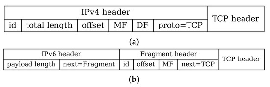
Figure 1.
Structure of fragmented IPv4 (a) and IPv6 (b) packets.
In IPv4, all relevant fields (contained in the IPv4 header) are:
- id—a 16-bit field identifying the fragment series;
- total length—length of the entire IP datagram;
- offset—a 16-bit data offset from the beginning of the original (not fragmented) IP packet;
- MF—“more fragments” flag indicating that this is not the last fragment;
- DF—“do not fragment” flag preventing fragmentation by gateways and routers;
- proto—type of the payload, e.g., TCP or UDP.
In the case of IPv6, some fields are moved to the fragment header (retaining similar semantics to IPv4). Overall, the relevant fields are:
- id—a 32-bit field identifying the fragment series;
- payload length—length of the payload (including extension headers);
- offset—a 16-bit data offset from the beginning of the original (not fragmented) IP packet;
- M—“more fragments” flag indicating that this is not the last fragment;
- next—type of the next header: e.g.,: TCP or UDP or an extension header.
The IPv6 protocol prevents fragmentation by the intermediate nodes, so a packet may be treated as having the flag. The source and destination address fields are left out from the picture as they require no explanation in this context. The fragment series is identified by the tuple:
- —for IPv4
- —for IPv6.
A fragment flow or a fragment series is thus uniquely identified by the tuple number 1 if the field is left “blank” for IPv6. Note that the bit width of the fields is different, so the implementation may choose to zero-extend the fields in the case of IPv4 to retain generality.
Figure 2 depicts a transformation process from a “whole” IPv4 packet to a fragment series. When a transmitting device detects that the IP datagram does not fit into the Maximum Transmission Unit (MTU), then the packet payload is split into several parts and each part gets its own IP header. If an original payload is 2000 bytes, then the size of an IPv4 packet is at least 2020 bytes due to the packet header overhead (the 20-byte length assumes no IP options in the header). Subsequently, two-part fragment series has 1520 and 520 bytes, respectively. In the case of IPv6, the overhead consists of the length of all the extension headers between the IPv6 packet header and the data beyond the extension header (there may be many extension headers). The last header in the series (containing the final bytes of the payload) has the flag (or for IPv6), thus indicating the final size of the packet.
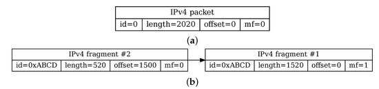
Figure 2.
A comparison of a defragmented IP packet (a) and corresponding fragment series (b).
Since IP delivery is not reliable, the packets may be reordered, dropped, or duplicated and the receiving node must attempt to reconstruct the original payload in all those cases. As a consequence, each fragment series must be buffered in the receiving device until a complete reconstruction is made. This process, if left uncompleted, is eventually interrupted by a timeout.
The process of IP reassembly is serviced by the flow table. A flow table is a lookup structure that keeps a state and payload for each active fragment flow. The data kept in the flow table should represent a sorted list of received fragments. When the list is complete, the original IP packet is reconstructed, and the entry is removed from the table. Figure 3 contains such a list (the length field is a payload-only length without the header overhead). The fragment series with id=0x100A has a known length, since the last part was received with . The total length is calculated as an offset of the last fragment (1800) plus its length. Since two previous packets contain only 1200 bytes, there are still 600 bytes lacking. The fragment series with id=0x1000B has an unknown length since there was no packet with .
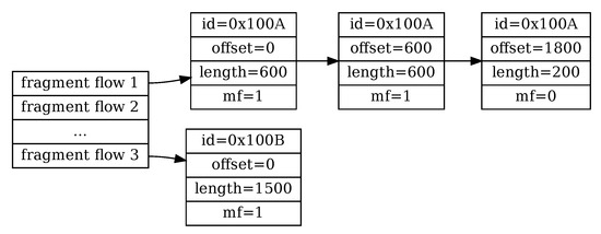
Figure 3.
IP Fragment table.
The IP defragmentation process follows the “best-effort” approach. A failed attempt to defragment an IP packet (e.g., due to lack of resources) is not considered fatal but should be avoided. In the Internet network architecture, it is the responsibility of a higher layer (TCP, DNS, etc.) to guarantee reliable delivery.
2.2. Network Traffic Statistics
Stateful traffic processing algorithms can vary in performance and resource consumption based on a statistical distribution of connections (flows) in the traffic. Real-world flow distribution in traffic has been characterized as highly skewed, long tail, and non-stationary by Adamic and Huberman [24]. There are noticeable small-scale phenomenons, such as burstiness as well as dependence on time of the day in the particular time zone. Both effects are well described in Ribeiro [25] and Benson [26]. Aggregated, high-bandwidth links were also extensively researched in Arfeen [27], where both small-scale and large-scale correlations can be detected. Fragmented IP traffic is a well-understood but somewhat marginal phenomenon in research due to the overall small share in Internet traffic bandwidth. The extensive analysis in Shannon [1] claims that it contributes to less than 1% of total traffic.
2.3. Flow State Memory and Caching
Stateful flow processing can be employed in various algorithms. One of the popular techniques is flow caching. Caching unicast routing decisions were demonstrated to be highly effective in Feldmeier [28]. It can speed up various networking algorithms such as label switching described in Kim [29] or OpenFlow rule processing in Congdon [16]. The design of OpenVSwitch, an open-source SDN forwarding plane described in Pfaff [30], is centered around the concept of caching. This technique is known to work well both in software and hardware. An example of a cache-based hardware architecture can be found in Okuno [31]. The advent of high-bandwidth fiber networks revived the interest in the energy efficiency of TCAM memory, which led Tanaka [15] to propose a flow cache as a means of reducing the TCAM hit rate. The general evaluation of flow cache memory performance is presented in Czekaj and Jamro [32], and subsequently, in Yamaki [14]. A recent example of using an FPGA-based Smart NIC for a flow-aware network processing can be found in Li [33].
2.4. Creating Synthetic Traffic in Networking
The need for creating synthetic traffic workloads has been well recognized in the industry. This is the basis of commercial network equipment testers such as IXIA [34] or Spirent [35]. A synthetic workload may be built out of real-world traffic samples containing single connections. Erlacher and Dressler [36] proposed using a mix of ordinary and attack payloads using the TRex traffic generator [37]. Gadelrab [38] used a similar technique for security research. Cerqueira [39] evaluated time series forecasting methods, showing that blocked cross-validation provides the best estimate of predicted performance for stationary time series and the second best one for a non-stationary case. This is especially relevant for networking as real-world traffic is proven to be non-stationary, as discussed in Arfeen [27] and Adamic and Huberman [24].
2.5. Summary of the Related Works
Table 2 presents a comparison of related works that focus on a flow table design. Most of the presented publications (except Tanaka [15]) concern a flow table of size of 1 K (one thousand entries) or less. The associativity is also similar (e.g., 2, 4, or 8) except of Congdon [16], which used small, fully associative Content-Addressable Memory (CAM). Two notable differences contribute to the novelty of this work. First is the testing method, which uses network samples in a novel way (see Section 2.4). Second is the protocol concerned, which is not a Layer 4 transport.
3. Materials and Methods
3.1. Software Simulation of the Ip Reassembly Module
3.1.1. Flow Table Design
The main subject of this work is to assess the required size (memory consumption) of an IP reassembly flow table required to keep the fragmented payload. The primary goal is a hardware design space exploration, the flow table is constructed in a hardware-friendly manner. The results do not lose generality as the same scheme (or even more sophisticated) can be efficiently implemented in software. The design attempts to maximize performance while keeping the memory organization simple and deterministic. This is especially important for high-speed fiber networks where the 100 Gb/s throughput (and beyond) mandates a pipelined architecture [15]. The conceptual organization of the flow table is presented in Figure 4. The main design factors are:
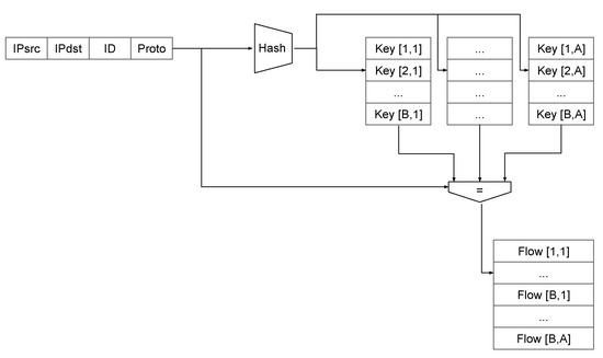
Figure 4.
Schematic of a flow table.
- Constant associativity A, which is a design parameter;
- Constant number of flow table entries , where B is a number of buckets or “sets” (also a design parameter);
- Least Recently Used (LRU) replacement policy based on a timestamp (e.g., a cycle or a packet counter).
The flow table design resembles the CPU data cache organization, hence the term “associativity” or “ways” is being preferred over the “bucket size” (used for hash tables). The address of the memory entry is generated by the hashing procedure, which is not present in data caches (which use a physical and virtual address as a key). The LRU policy is working within a “set” or a bucket. For example, for a four-way memory, the replacement policy can overwrite the oldest out of the four entries.
The main design challenge for such an algorithmic block is to choose a memory organization that is capable of holding all concurrent fragment flows without sacrificing too much silicon space. The rest of the article lays out the methodology and results of an experiment that systematically explores the solution space.
The IP reassembly algorithm has been implemented in software to perform a simulation of the proposed hardware block. Every attempt at implementing such a block in hardware should be preceded by algorithmic analysis.
An additional benefit of the simulation is that the results are applicable for software implementation as well. It can be safely assumed that a software variant can be much more sophisticated when it comes to control logic and thus outperform hardware on the algorithmic level (e.g., using cuckoo hashing or dynamic allocation). Thus, any benefit of this simulation can be applied to software with equal or even greater success.
Design space exploration parameters:
- Finite flow table with a predefined size in the range from 16 to 512 entries.
- Fixed associativity A from 1 to 16
- Infinite packet buffer space. Payload buffering limitations are not simulated.
- Constant 40-byte flow key constructed from .
- LRU replacement policy based on a timestamp.
- IP Fragments are properly defragmented even when they arrive out of order or duplicated.
- Infinite fragment list.
- No data flow modeling.
- No cycle-level modeling.
The size of the flow table (point 1) was chosen to be relatively small, which is typical for the network accelerators based on SRAM memory (e.g., Intel X700 [11]). Other hardware-oriented publications (e.g., Yamaki [14]) also consider the size in the order of a thousand entries.
Associativity of a table A defined in point 2 is an important parameter for the hardware design, as the complexity of implementation rises significantly beyond the four entries. Especially, the idealized LRU policy is often replaced by the pseudo-LRU, which is a design trade-off [40]. Furthermore, as discussed in Section 4, the benefits of increased associativity tend to diminish beyond 8.
Two design parameters, namely packet buffer space and fragment memory size (points 3 and 7) are considered “infinite”. This modeling practice is motivated by the need to limit the number of design parameters and focus only on the essential ones. The size of the buffer space strongly depends on the size of the flow table and can be estimated as , where is an average size of a defragmented (original) IP packet. Thus, the buffer space can be considered a dependent variable.
The fragment list size is an independent variable, but the proper value can be determined from the analysis of packet traces. This is done in Section 4.3.4. Since that value can be determined empirically, there is little incentive to assume it a priori.
The lack of data flow and cycle-level modeling stems from the standard hardware design practice. The key design parameters should be determined before the more detailed cycle-accurate model is implemented.
In summary, the main point of the simulation is to characterize the behavior of the flow table while ignoring or simplifying other aspects of the design.
3.1.2. Simulation System
The simulation system consists of several applications designed to work as a data pipeline. The schematic of the architecture can be found in Figure 5. The test design is generated and stored in a workflow definition (described in Section 3.2.2). Next, a test is constructed on the fly using a mixer application. A simulator accepts an input stream constructed by the mixer. The output of the simulation contains tables of network flows and cache events, which are stored for offline processing by statistical software. The essential parts of the process are described in Section 3.2.
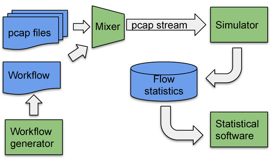
Figure 5.
Schematic of a simulation system.
3.2. Performance Estimation Methodology
3.2.1. Rationale
The methodology described in this section is originally designed to increase the robustness of simulation results and statistical estimates. Typical tests of network equipment are conducted using either simulated traffic or real-life packet traces. As noted in Section 2.4, there are hybrid approaches that use captured packet traces to construct specific tests.
The main drawback of the original data captured in the real network is that the fragmented packets are rare. Using some form of sample generation helps to overcome the limitation of insufficient bandwidth.
Synthetic data creation is popular among network security researchers (e.g., Gadelrab [38]). The machine learning (ML) community has also been using synthetic test creation to a great extent. This is a cornerstone of making ML systems more robust and prevent overfitting to the data. Randomized test creation ensures that ML systems and statistical inference tools capture the most important structure of the data while ignoring the accidental parts. Thus, cross-validation, split-validation, and derivatives are mandatory tools for both training and estimation [41,42].
The key observation is that a limited-size flow table with a replacement policy can be treated as an inference system or as a predictor. The overall simulation is a “model” that can be evaluated in the same manner as ML models. The only difference is the fact that the default LRU policy is fixed, so there is no training involved. Thus, the cross-validation technique can be used as a basis for constructing the validation test for a network processing model.
3.2.2. Test Generation
Deficiencies of traffic samples may stem from several factors:
- Abnormal network events captured in sampled traffic;
- Time-dependent traffic characteristics (network traffic from a single time zone follows daily and weekly patterns [26]);
- Insufficient bandwidth in the original sampled traffic;
- Operator-specific traffic profile.
The technique proposed below addresses all the issues above using a scheme similar to K-fold Cross-validation from ML field. Since the original method is sub-optimal for non-stationary time series [39], it has been adapted by mixing packet traces as opposed to creating a sequential vector. Algorithm 1 is a main test generation algorithm. Algorithm 2 is an address anonymization algorithm invoked by the main algorithm. Algorithm 3 is a traffic mixing algorithm invoked by the main part.
The prerequisites for an algorithm are as follows:
- —a set of all packet traces, each trace spans equal time;
- —a packet trace, i.e., a sequence of packets each with the associated timestamp , such that a first timestamp is 0 (the trace records only the relative time);
- M—the desired total number of tests;
- N—the number of packet traces forming a single test, ;
- —predefined IPv4 address constants.
The final remark about the algorithm is that the use of sampling makes the task of creating a test set somewhat independent (except due to the sampling without replacement) of the available number of traces as well as the individual trace size. Figure 6 depicts the process by showing that from packet traces there are M tests at the outcome, each consisting of N traces.
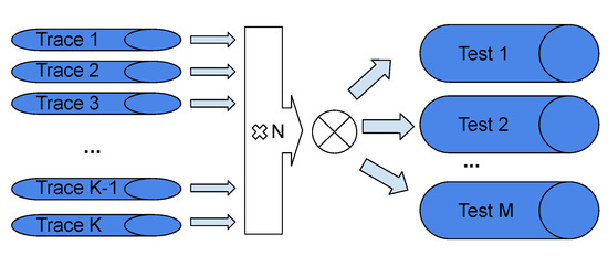
Figure 6.
Trace mixing schema.
3.2.3. Estimators and Confidence Intervals
The output of the simulation consists of M discrete statistics in a form of a cumulative distribution function (CDF). Each statistic from the test is an empirical CDF function . The function is a discrete cumulative “histogram” defined on L intervals such that each pair denotes observations of the random variable from the interval . The combined CDF function is a collection of all empirical CDFs from M tests.
For each of the L intervals , there is a collection of observations from M tests, which can be treated as a distribution of results. To produce a point estimate from M CDF functions, the mean and Confidence Interval (CI) estimates are computed for each interval.
The confidence interval estimate is calculated by estimating the 5th and 95th percentile of a sample distribution: . The quantile estimation method was chosen to be deleted Jackknife with random subsampling [43]. Appendix A describes this method in detail. It is a first-order accurate estimator (similar to bias-corrected bootstrap) [42] but less computationally intensive than bootstrap for a small sample size (less than 1000).
The exact choice of L and the exact number of intervals depends on the generated statistic. For Figure 7, Figure 8, and Figure 9a it follows the logarithmic scale:
where denotes the domain of the empirical CDF function from Equation (2).
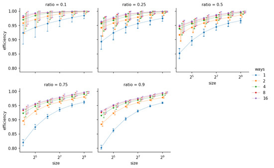
Figure 7.
Efficiency results as a function of number of entries in the flow table. Each sub-graph represents a different ratio of the test composition R. Each data series represents the flow table associativity A (number of ways). The X axis has logarithmic scale: .
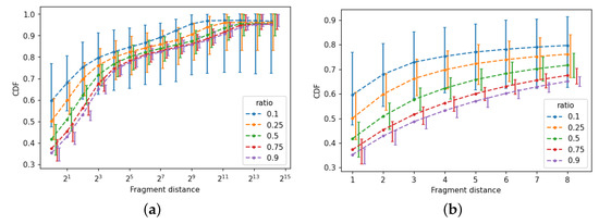
Figure 8.
Aggregate mean and confidence interval of cumulative distribution of packet fragment distance. (a) Whole range; (b) fragment distance up to 10.
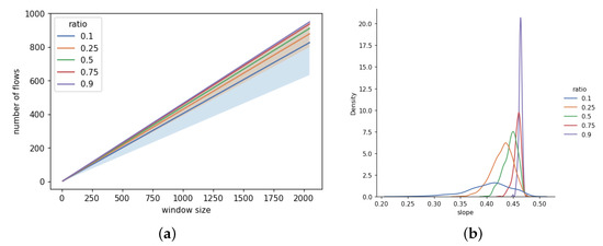
Figure 9.
(a) Linear fit of —a number of fragment flows as a function of packet window size. Shaded areas represent the two widest confidence regions of the slope. (b) The Gaussian kernel density estimation of the distribution of the slope a for each series.
4. Results
4.1. Data Sources
For the simulation, two popular network traffic datasets were extensively used:
- WAND, Waikato Internet Traffic Storage archives from WAND research group [44,45]. The traffic used in the paper comes from New Zealand’s Internet Service Provider (ISP) core router.
- MAWI, MAWI Working Group Traffic Archive [46,47]. This is the most recent traffic coming from a Japanese ISP’s backbone link.
Both datasets were explored in numerous publications, including those in Section 2 (e.g., Benson [26]).
4.2. Simulation Parameters
The simulation was configured as follows:
- The total number of traces is with each trace lasting 15 min
- −
- 130 packet traces from MAWI;
- −
- 93 traces from WAND with 30 min length were split into two halves, giving 186 traces, each lasting 15 min.
- The total number of individual tests was chosen as .
- Each individual test was a mix of , where R is a test composition ratio
- For each test run, the simulation program tested the following flow table parameters (see Figure 4):
- −
- The number of flow table entries is ;
- −
- The associativity (number of ways) .
The test composition ratio R deserves a longer explanation, as it controls the outcome of the simulation. Since the number of tests M is constant throughout the experiment, the ratio R determines the number N of packet traces being sampled (Algorithm 1) and mixed (Algorithm 3). As the ratio R increases up to , the number of tests increase up to M. The number of sampled and mixed tests have two consequences on the statistics obtained from the simulation:
- The bandwidth of a synthetic packet trace (mixed by Algorithm 3) increases with the ratio R. This is important in the case of IP fragmentation, as the original packet traces contain less than 1% of the relevant traffic.
- The statistical diversity (variance of the estimators) obtained from samples diminish as the R grows. This is observed empirically in Section 4.3 and can be deduced from the standard formula of a variance of a sample mean:
As a result, the choice of the constant M should be a function of the desired traffic bandwidth and variance of the results. Note that M is not dependent on the number of original samples K. Therefore, the choice of M can be arbitrary. This is a major advantage of such a sampling method over the traditional approach. It is somewhat analogous to the application of the bootstrap, which improves the robustness of any statistical estimator based on limited data on hand.
| Algorithm 1 Test generation. |
Require:S, M, N
|
| Algorithm 2 Trace anonymization |
function Anonymize()
|
| Algorithm 3 Trace mixing. |
function Mix(S)
|
4.3. Simulation Results
4.3.1. Efficiency
Figure 7 shows the efficiency metric collected among all test runs. The X axis is a table size (a number of entries), and the Y axis is the efficiency measured as a success rate.
where is a total number of complete (defragmented) IP packets and is a number of IP packets successfully defragmented by the given configuration (e.g., 16 entries one-way).
Efficiency data on Figure 7 demonstrates that higher bandwidth imposes more “stress” to the model, which results in lowering the efficiency (e.g., lowest score being 0.8 for vs. 0.92 for ) but at the same time reduces the spread of the results.
The main observation is that the efficiency results support the research hypothesis: the IP defragmentation algorithm is highly efficient with relatively small table size. If the one-way table is excluded from the consideration, the efficiency of 95% is reached with the table size of 128.
The second conclusion is that there are diminishing returns from increasing the associativity beyond 4. Technical challenges that haunt the highly associative memories increase the relevance of minimizing this parameter.
4.3.2. Intra-Arrival
Figure 8 displays the sample mean and confidence interval (CI) of intra-arrival count. This metric is a distance between two packet fragments from the same flow, so it is an indicator of traffic locality. For instance, a CDF value 0.6 for distance 8 means that in 60% of cases, the next packet from the same flow was at most eight packets apart. This chart demonstrates the effect of increasing the throughput of the packet traces used for testing. For example, for a distance of 1, which means that the next packet is from the same fragment flow, the possible range of values is between 0.35 for and 0.6 for .
The main conclusion from Figure 8 is that traffic locality is strong for all tests. Even accounting for confidence sets, there is at least a 50% chance that one of the next five packets is from the same flow, which can be derived from the lower confidence interval for series with .
The high traffic locality is the key to efficient flow processing and supports the results from Figure 7. The data should be interpreted as follows: fragmented IP packets are sent as a consecutive series of network frames and retain that property even in the aggregated traffic. This allows for processing them with relatively low memory consumption.
The notable trend that can be observed in Figure 8 and subsequent charts is that increasing the mix ratio R decreases the overall size of the confidence sets. This can be explained by the fact that the original diversity contained in the packet traces (smaller than synthetic) is recovered when the sampling ratio approaches 100%.
4.3.3. Flow Parallelism
In Figure 9, the number of flows in a packet window was approximated by a linear function for each of the data series associated with ratio R. The original metric measures how many unique flows can be found in a rolling window of a certain size.
where is a ith packet in a trace, w is a packet window of size n, and is a flow counting function. This metric can be interpreted as a measure of “flow parallelism”, i.e., how many flows are “active” in the same unit of time.
For a single test, a single window of size n produces a population of measurements, i.e., is a sampled random variable. So, the final metric computesthe 95th percentile of all measurements for n. For example, a window of 256 with a number of flows 100, that is, = 100, means that in 95% cases in 256 consecutive packets there are no more than 100 unique IP fragment flows. Since there are M tests, the estimate is itself a population sample, i.e., there are M samples of for each data series in Figure 9.
The point measurements are approximated by using the least squares method (constant term, a.k.a. intercept, is fixed at 0). The slope coefficient a for each data set is slightly different, so Figure 9a displays the mean slope for each series of M tests along with the two biggest confidence regions. Each data series represents all tests created with the same ratio of tests R. The detailed results of the linear fit can be found in Table 3. The minimal coefficient of determination is defined as
where are samples, is an approximating function and is a variance estimator. is more than 0.97 for all cases (shown in Table 3), which suggests a strong linear relationship (at least 97% of the variance is explained by the linear function ). Figure 9b shows the Gaussian kernel density estimate of the distribution of the slope parameter a. The variance becomes smaller with the growing number R. None of the probability mass functions can pass a t-test for identity with any other. The p-value is negligible for all pairs of distributions (less than ).
Table 3.
Linear fit results for Figure 9.
Measuring the flow parallelism provides additional evidence for flow locality. Highly local traffic should have lower for a given n than non-local traffic.
Figure 9b shows the relation between mix ratio R and the distribution of the slope of in the samples. The differences between slope distributions are consistent with the previous metrics, e.g., intra-arrival. That is, the variance becomes smaller with higher R.
4.3.4. Flow Length
Figure 10 represents a histogram of a sample mean of packet count in a single IP fragment flow. The expected number of fragments is 2, while the most extreme cases reach 8 packets and more. This follows the findings from Shannon et al. [1]. The higher number of packets in the fragment series most likely indicates an invalid flow (it can be a part of a DDOS attack or a firewall evasion technique). Fragment flows with packet count 1 are incomplete and cannot be reassembled.
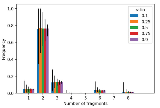
Figure 10.
Histogram of the sample mean and the confidence intervals of the fragment count. Each data series represents a different ratio R.
The distribution of the flow length can be used to resolve the question from Section 3.1.1 about the fragment list size. Since the expected fragment length seldom exceeds 8, the list length of 8 should suffice for practical implementation.
5. Discussion
5.1. Simulation Results
The results from Section 4 indicate that the initial hypothesis of high-traffic locality holds for a wide range of tests with real-world data. Furthermore, the amount of flow memory needed to successfully reassemble most of the IP fragments does not have to be large. The number of ways should be no less than 4 and no more than 16, while the flow table size should be 128 or larger. That parameter range yields at least 95% effectiveness across tests.
5.2. Methodology
The original methodological approach undertaken for this particular simulation experiment deserves an independent assessment. The main conclusion from the large-scale traffic mixing experiment is that it allows the range of tests or simulations to be “enriched” in the case of an insufficient number of original test samples or when individual sample diversity is unsatisfactory. The mixing ratio R plays a crucial role in controlling the variance of the results. Choosing an R that is too high may result in a large number of traffic tests that are highly similar to each other. If the main purpose of such an experiment is parameter tuning, this may lead to “overfitting” (this hypothesis is beyond the scope of this work).
The randomized nature of the original sample selection for mixing should be controlled by “seeding” the random number generator. This ensures that individual tests are reproducible and do not need to be stored but can be generated on the fly. This gives an additional benefit of making the storage space independent of the total number of tests (but rather on the number of original samples). This is not a trivial problem as packet traces from high-speed networks can easily consume terabytes of storage. The obvious cost of a large number of tests is the amount of computing power that in this particular case approached hundreds of CPU hours. The recommended way to tackle this problem is to run many test cases in parallel on a computing cluster or a high-end multi-core platform.
5.3. Future Work
The sample generation technique presented in this paper can be adapted to a wide range of simulation problems, such as design space search for algorithms, hardware model verification, or fuzzing software systems (randomized test generators). Network-oriented machine learning algorithms is a growing and popular field, which could directly benefit from large-scale packet sample synthesis. However, it is still undetermined how this particular method affects the supervised learning process or out-of-sample verification.
An obvious research direction when it comes to IP defragmentation is a replacement policy employed be the flow table. Some research mentioned in Section 2 (e.g., Yamaki [14]) was exclusively focused on developing a technique that can beat the LRU either in performance or resource efficiency. Since the problem of IP defragmentation is somewhat different from connection tracking (as discussed in Section 1.3), it deserves an independent assessment of cache replacement policies.
Author Contributions
Conceptualization, M.C., E.J., and K.W.; methodology, M.C. and E.J.; software, M.C.; validation, M.C.; formal analysis, M.C. and E.J.; investigation, M.C.; resources, E.J., K.W.; data curation, M.C.; writing—original draft preparation, M.C.; writing—review and editing, E.J. and K.W.; visualization, M.C. and E.J.; supervision, K.W.; project administration, K.W.; funding acquisition, K.W. All authors have read and agreed to the published version of the manuscript.
Funding
This research received no external funding.
Data Availability Statement
All data sets used in this work are cited and publicly available (see Section 4.1).
Conflicts of Interest
The authors declare no conflict of interest.
Acronyms
| CAM | Content-Addressable Memory |
| CDF | Cumulative Distribution Function |
| CI | Confidence Interval |
| CI | Confidence Interval |
| DPI | Deep Packet Inspection |
| FPGA | Field Programmable Gate Array |
| IDS | Intrusion Detection System |
| ISP | Internet Service Provider |
| LRU | Least Recently Used |
| MTU | Maximum Transmission Unit |
| NIC | Network Interface Card |
| SDN | Software-Defined Networking |
| SOC | System On Chip |
| SRAM | Synchronous Random Access Memory |
| TCAM | Ternary Content-Addressable Memory |
| TLS | Transport Layer Security |
Glossary
| MPLS/GRE | A tunnel protocol based on Multi Protocol Label Switching (MPLS) and Greneric Routing Encapsulation(GRE) |
| HBM2 | High Bandwidth Memory, an on-chip dynamic RAM optimized for high bandwidth. Puplar in Graphics Prosessing Units (GPUs) and high-end FPGAs |
| DDOS | Distributed Denial of Service attack, a massive request stream aimed at overwhelming the network service originated from many (geographically distributed) clients |
Appendix A. Estimation Method
Let denote the collection of independent and identically distributed (i.i.d.) samples. Let be a statistic of interest. The variance estimator of a statistic is based on computing a statistic by generating subsets of all samples of size (d is the number of deleted samples in a single set). There are possible subsets s, so full estimation may be computationally more expensive than bootstrap, which typically uses a constant number of subsets from 1000 to 10,000 [41]. However, the collection of N statistics can also be sampled, in which case the method is called “random subsampling”. The method draws a random sample with replacement from S and estimates by
where
In order to retain consistency of the estimator, the numbers m and d should be chosen so that is bounded while [43,48]. The term is an estimate of a statistic obtained by a sample mean and is a variance correction term. Since the Jackknife estimator approximates the normal distribution, the confidence interval can be computed using the Student approximation of the normal. The confidence interval can be obtained by
where is the inverse Student CDF.
References
- Shannon, C.; Moore, D.; Claffy, K.C. Beyond folklore: Observations on fragmented traffic. IEEE/Acm Trans. Netw. 2002, 10, 709–720. [Google Scholar] [CrossRef]
- Rescorla, E. The Transport Layer Security (TLS) Protocol Version 1.3; 2018; Available online: https://datatracker.ietf.org/doc/html/rfc8446 (accessed on 8 April 2021).
- Kent, S.; Seo, K. Security Architecture for the Internet Protocol; RFC 4301; 2005; Available online: http://www.rfc-editor.org/rfc/rfc4301.txt (accessed on 8 April 2021).
- Worster, T.; Rekhter, Y.; Rosen, E. Encapsulating MPLS in IP or Generic Routing Encapsulation (GRE); RFC 4023; 2005; Available online: https://www.rfc-editor.org/rfc/rfc4023.html (accessed on 8 April 2021).
- Mahalingam, M.; Dutt, D.; Duda, K.; Agarwal, P.; Kreeger, L.; Sridhar, T.; Bursell, M.; Wright, C. Virtual eXtensible Local Area Network (VXLAN): A Framework for Overlaying Virtualized Layer 2 Networks over Layer 3 Networks; RFC 7348; 2014; Available online: http://www.rfc-editor.org/rfc/rfc7348.txt (accessed on 8 April 2021).
- Holz, R.; Hiller, J.; Amann, J.; Razaghpanah, A.; Jost, T.; Vallina-Rodriguez, N.; Hohlfeld, O. Tracking the deployment of TLS 1.3 on the Web: A story of experimentation and centralization. ACM Sigcomm Comput. Commun. Rev. 2020, 50, 3–15. [Google Scholar] [CrossRef]
- Kunz, A.; Salkintzis, A. Non-3GPP Access Security in 5G. J. ICT Stand. 2020, 8, 41–56. [Google Scholar] [CrossRef]
- Bonica, R.; Baker, F.; Huston, G.; Hinden, B.; Troan, O.; Gont, F. IP Fragmentation Considered Fragile; Technical Report, IETF Internet-Draft (Draft-Ietf-Intarea-Frag-Fragile), Work in Progress…; 2019; Available online: https://datatracker.ietf.org/doc/rfc8900/ (accessed on 8 April 2021).
- Intel. Intel® FPGA Programmable Acceleration Card N3000 for Networking. 2016. Available online: https://www.intel.com/content/dam/www/programmable/us/en/pdfs/literature/po/intel-fpga-programmable-acceleration-card-n3000-for-networking.pdf (accessed on 8 April 2021).
- NVidia. ConnectX-6 DxDual-Port 100GbE/Single-Port 200GbE SmartNIC. 2021. Available online: https://www.mellanox.com/products/ethernet-adapters/connectx-6-dx (accessed on 8 April 2021).
- Intel. Intel® XL710 40 GbE Ethernet Adapter. 2016. Available online: https://i.dell.com/sites/csdocuments/Shared-Content_data-Sheets_Documents/en/us/Intel_Dell_X710_Product_Brief_XL710_40_GbE_Ethernet_Adapter.pdf (accessed on 8 April 2021).
- Marvell. Marvell® Infrastructure Processors. 2021. Available online: https://www.marvell.com/products/infrastructure-processors.html (accessed on 8 April 2021).
- Xilinx. Xilinx Alveo Adaptable Accelerator Cards for Data Center Workloads. 2021. Available online: https://www.xilinx.com/products/boards-and-kits/alveo.html (accessed on 8 April 2021).
- Yamaki, H. Effective cache replacement policy for packet processing cache. Int. J. Commun. Syst. 2020, 33, e4526. [Google Scholar] [CrossRef]
- Tanaka, K.; Yamaki, H.; Miwa, S.; Honda, H. Evaluating architecture-level optimization in packet processing caches. Comput. Networks 2020, 181, 107550. [Google Scholar] [CrossRef]
- Congdon, P.T.; Mohapatra, P.; Farrens, M.; Akella, V. Simultaneously reducing latency and power consumption in openflow switches. IEEE/ACM Trans. Netw. (TON) 2014, 22, 1007–1020. [Google Scholar] [CrossRef]
- Postel, J. Internet Protocol; STD 5; 1981; Available online: http://www.rfc-editor.org/rfc/rfc791.txt (accessed on 8 April 2021).
- Touch, J. Updated Specification of the IPv4 ID Field; RFC 6864; 2013; Available online: http://www.rfc-editor.org/rfc/rfc6864.txt (accessed on 8 April 2021).
- Deering, S.; Hinden, R. Internet Protocol, Version 6 (IPv6) Specification; STD 86; 2017; Available online: https://www.omgwiki.org/dido/doku.php?id=dido:public:ra:xapend:xapend.b_stds:tech:ietf:ipv6 (accessed on 8 April 2021).
- NXP. Overview of Autonomous IPSec with QorIQT Series Processors. 2014. Available online: https://www.nxp.com/files-static/training/doc/ftf/2014/FTF-NET-F0111.pdf (accessed on 8 April 2021).
- Lin, V.; Manral, V. Methods and Systems for Fragmentation and Reassembly for IP Tunnels in Hardware Pipelines. U.S. Patent App. 11/379,559, 23 April 2006. [Google Scholar]
- Zhao, Y.; Yuan, R.; Wang, W.; Meng, D.; Zhang, S.; Li, J. A Hardware-Based TCP Stream State Tracking and Reassembly Solution for 10G Backbone Traffic. In Proceedings of the 2012 IEEE Seventh International Conference on Networking, Architecture, and Storage, Xiamen, China, 28–30 June 2012; pp. 154–163. [Google Scholar]
- Ruiz, M.; Sidler, D.; Sutter, G.; Alonso, G.; López-Buedo, S. Limago: An FPGA-Based Open-Source 100 GbE TCP/IP Stack. In Proceedings of the 2019 29th International Conference on Field Programmable Logic and Applications (FPL), Barcelona, Spain, 9–13 September 2019; pp. 286–292. [Google Scholar] [CrossRef]
- Adamic, L.; Huberman, B. Zipfs law and the internet. Glottometrics 2002, 3, 143–150. [Google Scholar]
- Ribeiro, V.J.; Zhang, Z.L.; Moon, S.; Diot, C. Small-time scaling behavior of Internet backbone traffic. Comput. Netw. 2005, 48, 315–334. [Google Scholar] [CrossRef] [Green Version]
- Benson, T.; Akella, A.; Maltz, D.A. Network Traffic Characteristics of Data Centers in the Wild. In Proceedings of the IMC ’10: 10th ACM SIGCOMM Conference on Internet Measurement, Melbourne, Australia, 1–30 November 2010; Association for Computing Machinery: New York, NY, USA, 2010; pp. 267–280. [Google Scholar] [CrossRef]
- Arfeen, M.A.; Pawlikowski, K.; Willig, A.; Mcnickle, D. Internet traffic modelling: From superposition to scaling. IET Netw. 2014, 3, 30–40. [Google Scholar] [CrossRef]
- Feldmeier, D.C. Improving Gateway Performance with a Routing-Table Cache. In Proceedings of the IEEE INFOCOM’88, Seventh Annual Joint Conference of the IEEE Computer and Communcations Societies, Networks: Evolution or Revolution? New Orleans, LA, USA, 27–31 March 1988; pp. 298–307. [Google Scholar]
- Kim, N.; Jean, S.; Kim, J.; Yoon, H. Cache replacement schemes for data-driven label switching networks. In Proceedings of the 2001 IEEE Workshop on High Performance Switching and Routing (IEEE Cat. No.01TH8552), Dallas, TX, USA, 29–31 May 2001; pp. 223–227. [Google Scholar] [CrossRef]
- Pfaff, B.; Pettit, J.; Koponen, T.; Jackson, E.; Zhou, A.; Rajahalme, J.; Gross, J.; Wang, A.; Stringer, J.; Shelar, P.; et al. The Design and Implementation of Open vSwitch. In Proceedings of the 12th USENIX Symposium on Networked Systems Design and Implementation (NSDI 15), Oakland, CA, USA, 4–6 May 2015; USENIX Association: Oakland, CA, USA, 2015; pp. 117–130. [Google Scholar]
- Okuno, M.; Nishimura, S.; Ishida, S.I.; Nishi, H. Cache-based network processor architecture: Evaluation with real network traffic. IEICE Trans. Electron. 2006, 89, 1620–1628. [Google Scholar] [CrossRef]
- Czekaj, M.; Jamro, E. Flow caching effectiveness in packet forwarding applications. Comput. Sci. 2019, 20. [Google Scholar] [CrossRef]
- Li, J.; Sun, Z.; Yan, J.; Yang, X.; Jiang, Y.; Quan, W. DrawerPipe: A Reconfigurable Pipeline for Network Processing on FPGA-Based SmartNIC. Electronics 2020, 9, 59. [Google Scholar] [CrossRef] [Green Version]
- Technologies, K. Network Visibility and Network Test Products. 2021. Available online: https://www.keysight.com/zz/en/cmp/2020/network-visibility-network-test.html (accessed on 8 April 2021).
- Spirent. High-Speed Ethernet Testing Solutions. 2021. Available online: https://www.spirent.com/solutions/high-speed-ethernet-testing (accessed on 8 April 2021).
- Erlacher, F.; Dressler, F. Testing ids using genesids: Realistic mixed traffic generation for ids evaluation. In Proceedings of the ACM SIGCOMM 2018 Conference on Posters and Demos, Budapest, Hungary, 20–25 August 2018; pp. 153–155. [Google Scholar]
- Cisco. TRex Realistic Traffic Generator. Available online: https://trex-tgn.cisco.com/ (accessed on 8 April 2021).
- Gadelrab, M.; Abou El Kalam, A.; Deswarte, Y. Manipulation of network traffic traces for security evaluation. In Proceedings of the 2009 International Conference on Advanced Information Networking and Applications Workshops, Bradford, UK, 26–29 May 2009; pp. 1124–1129. [Google Scholar]
- Cerqueira, V.; Torgo, L.; Mozetič, I. Evaluating time series forecasting models: An empirical study on performance estimation methods. Mach. Learn. 2020, 109, 1997–2028. [Google Scholar] [CrossRef]
- Sudarshan, T.; Mir, R.A.; Vijayalakshmi, S. Highly efficient LRU implementations for high associativity cache memory. In Proceedings of the 12 International Conference on Advances in Computing and Communications, ADCOM-2004, Ahmedabad, India, 15–18 December 2004; pp. 24–35. [Google Scholar]
- Efron, B.; Hastie, T. Computer Age Statistical Inference; Cambridge University Press: Cambridge, UK, 2016; Volume 5. [Google Scholar]
- Efron, B.; Tibshirani, R.J. An Introduction to the Bootstrap; CRC Press: Boca Raton, FL, USA, 1994. [Google Scholar]
- Young, G. 15. The Jackknife and Bootstrap. J. R. Stat. Soc. Ser. A (Stat. Soc.) 1996, 159, 631–632. [Google Scholar] [CrossRef]
- WITS: Waikato INTERNET Traffic Storage. 2013. Available online: https://wand.net.nz/wits/ (accessed on 8 April 2021).
- Cleary, J.; Graham, I.; McGregor, T.; Pearson, M.; Ziedins, L.; Curtis, J.; Donnelly, S.; Martens, J.; Martin, S. High precision traffic measurement. IEEE Commun. Mag. 2002, 40, 167–173. [Google Scholar] [CrossRef]
- WIDE Project. 2020. Available online: http://mawi.wide.ad.jp/mawi/ (accessed on 8 April 2021).
- Sony, C.; Cho, K. Traffic data repository at the WIDE project. In Proceedings of the USENIX 2000 Annual Technical Conference: FREENIX Track, San Diego, CA, USA, 18–23 June 2000; pp. 263–270. [Google Scholar]
- Politis, D.N.; Romano, J.P. Large sample confidence regions based on subsamples under minimal assumptions. Ann. Stat. 1994, 22, 2031–2050. [Google Scholar] [CrossRef]
Publisher’s Note: MDPI stays neutral with regard to jurisdictional claims in published maps and institutional affiliations. |
© 2021 by the authors. Licensee MDPI, Basel, Switzerland. This article is an open access article distributed under the terms and conditions of the Creative Commons Attribution (CC BY) license (https://creativecommons.org/licenses/by/4.0/).