Classification of Microscopic Laser Engraving Surface Defect Images Based on Transfer Learning Method

Abstract

Microscopic laser engraving surface defect classification plays an important role in the industrial quality inspection field. The key challenges of accurate surface defect classification are the complete description of the defect and the correct distinction into categories in the feature space. Traditional classification methods focus on the terms of feature extraction and independent classification; therefore, feed handcrafted features may result in useful feature loss. In recent years, convolutional neural networks (CNNs) have achieved excellent results in image classification tasks with the development of deep learning. Deep convolutional networks integrate feature extraction and classification into self-learning, but require large datasets. The training datasets for microscopic laser engraving image classification are small; therefore, we used pre-trained CNN models and applied two fine-tuning strategies. Transfer learning proved to perform well even on small future datasets. The proposed method was evaluated on the datasets consisting of 1986 laser engraving images captured by a metallographic microscope and annotated by experienced staff. Because handcrafted features were not used, our method is more robust and achieves better results than traditional classification methods. Under five-fold-validation, the average accuracy of the best model based on DenseNet121 is 96.72%.

1. Introduction

Laser engraving technology is one of the most commonly used and efficient methods to improve the resistance of electrical connection devices. With the development of the mobile Internet, this technology has been more and more widely used on the electrical connection surface of mobile phone shells. The resistance stability of the electrical connection device in the mobile phone shell is the key to the normal signal reception of the mobile phone. Therefore, a simple and efficient surface defect classification method has great significance in the industrial field.

The image detection technology method is the most commonly used detection method in the industrial field [1]. The development and integration of image acquisition and processing technology have resulted in the great success of automatic inspection technology in the field of quality monitoring and non-destructive testing. Automated detection technology combines machine learning technology and deep learning technology. The algorithm can greatly improve the detection efficiency while meeting the detection requirements of high accuracy and low error rate. Convolutional neural network is the most commonly used technique in defect detection technology. It does not need feature extraction and image processing, because these capabilities are embedded in the hidden layer. Manual inspection of laser engraved film microscopic images increases the inspection time and reduces the accuracy rate [2]. The manual inspection ability will be exhausted with dim and endless work. The application of machine learning and deep learning technology to defect detection not only reduces the labor burden of workers, but also improves detection efficiency, matching high production with high detection rate.

Jiang [3] used the decision tree to classify the defects on the gold-plated contact surface of a printed circuit board (PCB). Moreover, bootstrap sampling technology was used to solve the small sample problem and minimize over-fitting. The experimental results show that the decision tree could classify samples and the accuracy rate was 97.87%. Its classification performance is better than the clustering algorithm and nearest neighbor classification. However, the expansion performance of the decision tree is limited and cannot be well applied to other different production scenarios. Kim [4] modified the decision tree to classify the chips of dynamic random-access memory. He first binarized the wafer diagram, input the decision tree for classification according to the shape pattern and defect location of the binary diagram and, finally, achieved an average accuracy of 95.6%. Nevertheless, their study considered only four models, not all possible models. Kang [5] used random forest to predict the defects of bare wafer. He used three characteristic parameters: the distance between bare wafer and wafer center, wafer test failure rate and deformation degree of wafer diagram. It was found that this method has some disadvantages. Some of the three characteristic parameters are not important, resulting in a waste of training time, and important manufacturing data are not used in this study. Baly [6] used high-dimensional hyperplane to classify wafer data. This method can effectively classify multi-modal, multi parameter and indivisible wafer data points. In the experiment, the partial least square method, general regression network and nearest neighbor method are used to compare and evaluate their models. The experimental results show that a support vector machine is better than other classifiers. However, the author only classified it as good or bad and did not analyze the causes of defects. Ooi [7] used an adjustable decision tree to identify multi-mode defects and solved the decision tree phenomenon of empty leaf nodes. This phenomenon occurs when there is an effective path but there is no associated learning sample, which eventually produces an instance without classification. Kuo [8] used two multilayer perceptrons to study five defect types in LED chips. They adopted four features: area, perimeter, tightness and defect rate. These features were extracted and sent to the first MLP to determine whether there was a defect and the second MLP (multilayer perceptron) determined the defect type. The overall recognition rate reached 97.83%. Sun [9] compared the performance of MLP and LVQ (learning vector quantization) network models in four thermal fuse defects classification. He used threshold and morphology to extract four defect features and feed them into two classifiers. The experimental results show that MLP had better accuracy than LVQ, but the time consumed by LVQ is less than MLP. Chiou [10] used two MLPs to detect defects in the gold-plated area of a printed circuit board. The first MLP was used to identify the pixels where the gold-plated area was located and the second MLP was used to classify specific defects. The accuracy of the network was 96% but this method could not recognize the image connected with the defect and the area without gold plating. Bilal [11] presented an infrared assisted thermal vulnerability detection technique, which applied affine transform to multimodal image fusion. It could accurately locate the hot center and obtain the spatial information of the component. The technology provided a reliable automated identification of hot spots in the system. Lu [12] proposed a publicly available multimodal printed circuit board dataset, FICS-PCB, for automated visual inspection of printed circuit boards. Mukhil [13] proposed an electronic component localization and detection network to detect the defects of PCB components and, finally, achieved a good performance of 87.2% accuracy and 98.9% recall. Most of the above methods use traditional statistical methods to detect defects in the collected natural images. They mainly extract several specific manual features, resulting in incomplete feature extraction or non-extraction of key features, which poses great challenges to defect detection. In addition, there are many interference noises in the natural images, which is not conducive to subsequent feature extraction.

In this work, we innovatively use laser engraving microscope images for surface defect classification. We used the metallographic microscope to collect the image of the radium carving position in the mobile phone shell, labelled by quality inspection workers. We took pictures in different light fields to imitate actual production environment and different types of laser engraving surface. In this specific industrial application field, it is very meaningful to propose an accurately labeled and high-quality image dataset that can be used for deep learning model training.

We designed a high accuracy microscopic laser engraving surface defect detection algorithm through two comparison experiments using transfer learning methods, which greatly saves the cost of labeling and training time without compromising the performance of the model. We discussed the detection performance of the VGG19, ResNet50, DenseNet121 and InceptionV3 networks under two different fine-tuning models. The results show that deep fine-tuning models had better effect compared with shallow fine-tuning, except VGG19. Then, we made a comparison of the accuracy of deep learning methods and two machine learning detection methods. The best accuracy, of 96.72%, was achieved under deep learning methods. Besides, the proposed algorithm was applied to production detection equipment and achieved good application results.

The remaining paper is organized as follows: Section 2 introduces the application of machine learning and deep learning in defect detection. Section 3 presents various convolutional network structures and the experimental method used in this paper. Section 4 summarizes the experiments and discusses the results. Section 5 concludes our work and prospects future research.

2. Related Works

2.1. Machine Learning Methods

Traditional machine learning methods include feature extraction and classification. The challenge of it is to artificially find a feature that can depict defects completely. Defect classification uses many image features. They include linear decomposition methods [14,15], Gabor filters [16], fast Fourier transform (FFT) [17], wavelet transform [18], gray-level co-occurrence matrix (GLCM) [19] and local binary pattern (LBP) [20]. Many classification methods can be selected once the features are determined and they include a support vector machine (SVM) [21], decision tree [22] and random forest [23]. The SVM classifier can find a hyperplane where the maximum separation separates the two classes. It is only suitable for classifying linearly distributed data. SVMs were extended to non-linear spaces very early, in 1996. I would just cite extended SVM with the work by Vapnik and colleagues [24].

The machine learning method is a short-term method that is often used in industrial inspections. Sindagi et al. used two different extraction modules to extract different defective features of OLED panels and feed the feature vector into the classifier [25]. Huang used GLCM to combine multiple features for WBMs [26]. Liao used the SVM classifier to classify the patterns obtained through morphological methods based on real wafer data [27]. The results show that the method achieved a global 95% correct rate and 5% false alarm rate. However, there was only a 72% accuracy for some circular and repeated scratches. Chang et al. achieved a high accuracy in the camera lens classification task. He detected five feature vectors and used SVM for classification. However, due to the narrow area and low-intensity contrast, some defects could not be detected. It was observed that SVM performed well in binary classification tasks.

2.2. Deep Learning Methods

Convolutional neural networks (CNNs) are specialized in dealing with image classification due to the hidden layers for feature extraction [28]. With the development of powerful GPU computing, a new generation of automatic image detection systems has appeared in the industrial field, showing superior performance, which includes application in surface defects of LED chips [29], computer-aided detection of gold-plated areas [10] and automatic detection of semiconductor wafers [30]. Although CNN has shown good performance in these applications, it has a disadvantage that it needs a lot of sample data, which is difficult to satisfy in industrial scenarios.

Research suggests that transfer learning can perform well even in small sample datasets. CNNs can transfer the pre-trained weights of large dataset to a small one. The key lies in the similarity between the two datasets [31]. Although there is little similarity between original images and industrial images, experiments have shown that transfer learning has great potential in industrial imaging.

There are two approaches to transfer learning. The first one takes pre-trained CNN as feature extractor. Specially, the pre-trained network is used to obtain features, then feed them into a classifier [32]. The second group adjusts the pre-trained network to suit the application, for instance, by modifying the last output layer to logical output, then using the labeled data to train different layers. Specially, there are two common training strategies. One is to train only the fully connected layers and keep the rest of the network the same and the other is to train the whole network. The transfer learning approach has achieved excellent results on lots of datasets [33,34,35,36]. Hua Yang et al. suggested the use of a pretrained network for mura defect classification [37]. Kazunori proposed a two-stage method, pre-training and fine-tuning for classification [38]. Thousands of data are used to train the first parameters of CNN, including some wrong labels due to weakly supervised training. The second parameters of pre-final-layers are trained from a small amount of data with high reliability. The feature extractor obtained by transfer learning can extract general features suitable for different tasks. Transfer learning provides a new idea to extract features for laser engraving defects classification.

3. Proposed Method

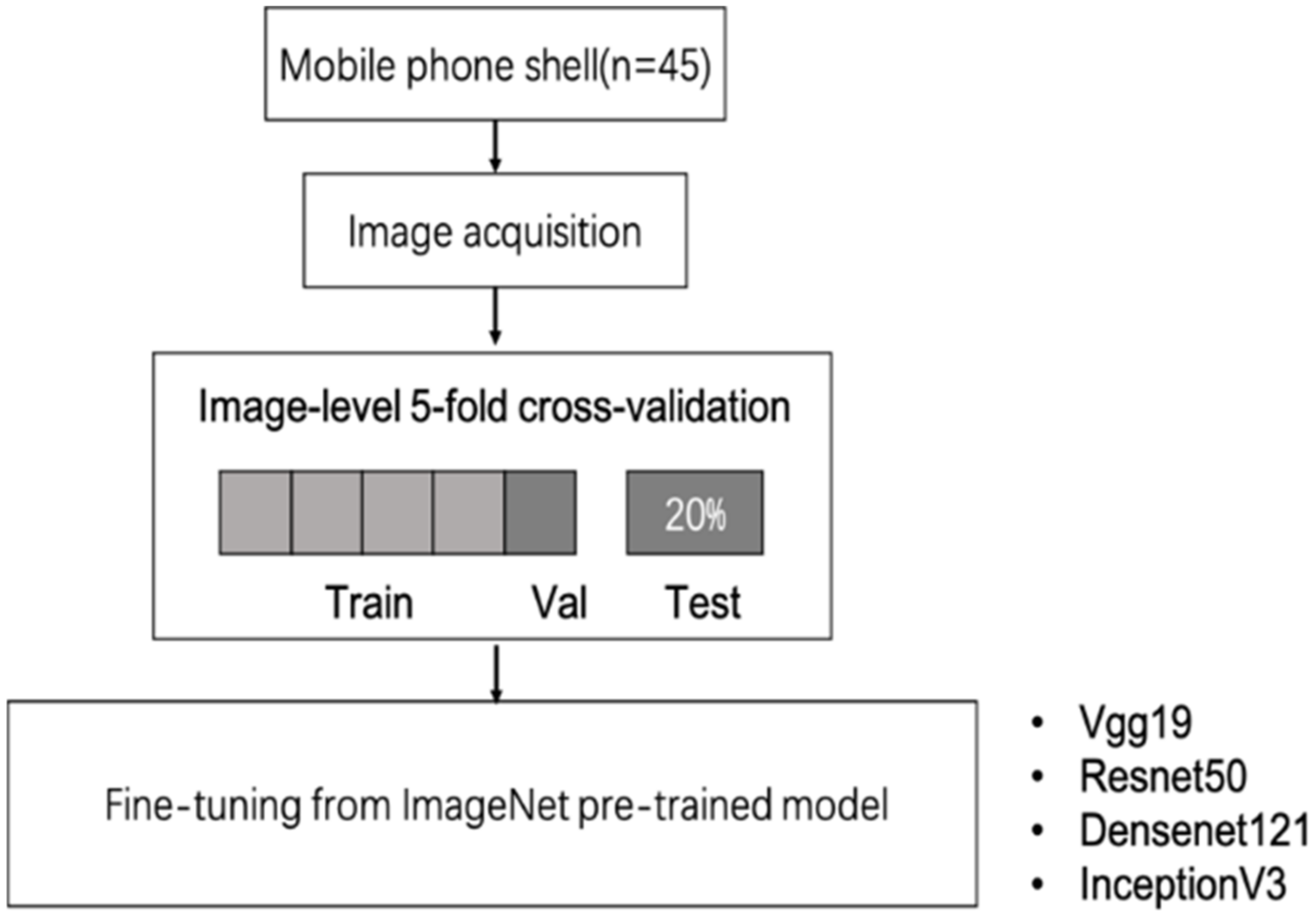
3.1. Overview of Method

The study design, including image acquisition, cross-validation and different fine-tuning strategies, is shown in Figure 1. Image acquisition was conducted on the mobile phone shell. Then, we divided the data into three parts for train, validation and test. Five-fold cross-validation was used on the dataset. Finally, the performance of VGG19, ResNet50, DenseNet121 and InceptionV3 were explored and evaluated by different fine-tuning strategies from pre-trained models.

3.2. Dataset

In this research, we used the metallographic microscope to collect the image of the radium carving position in the mobile phone shell. In order to prevent repeated acquisition, as shown in Figure 2, we labelled each laser carving position. We took pictures in different light fields to imitate actual production environment.

The metallographic microscopy system used in this project to collect the microscopic images of laser engraving on the mobile phone shell was an Aosvi professional metallographic microscope. The industrial camera was an Aosvi M140 camera, which supported USB2.0 interface and had the highest resolution of 4096 × 3288; real-world units was 5.73 μm × 4.60 μm. The resolution could make the surface of the laser engraving microscopic image clearly visible and achieve the required effect for classification. The metallographic microscope adopted falling illumination system, the light source was a 6 V/20 W halogen lamp and brightness was adjustable. According to the practical application of complex environment, such as different characteristics of light source, we used different yellow and green filters for the experiments. In the process of laser engraving, regular small space units are formed on the metal surface due to high-energy laser irradiation. The diameter of these units is very small, so the metallographic microscope magnification was set at 200 times, meeting the demand of classification.

The dataset contained four types of laser engraving surface (i.e., defect-free, irregular, black hole and large cell spacing, as shown in Figure 1) from 45 mobile phone shell with a total of 1986 images. The size of each image was 3664 × 2748 pixels. We used nearest neighbor interpolation transformation to adjust the image size to 224 × 224 to meet the input of CNN.

Figure 3 shows the types of laser engraving defects. Defect-free laser carving has a regular appearance. The defect types are that there are many black holes on the surface of laser carving, the spacing among laser carving units is large, the shape of laser carving is irregular and there are non-lasing areas.

We used a metallurgical microscope to capture laser engraving microscopic images under different lighting environments. A database was established for future training and testing. We used the fine-tuning method to extract features and retain useful features. Moreover, we used a fully connected layer to classify features; then, we compared the results among different fine-tuning strategies. The experimental results indicate that the all-layer fine-tuning method was superior to the training-only of fully connected layers.

3.3. CNN Models

Different convolutional neural network structures bring different feature extraction effects. Generally, more complex features can be extracted with the increase of the network. However, the specific network to choose depends on different datasets. In this paper, four networks with different structures were selected for comparative experiments.

On the ImageNet Large Scale Visual Recognition Challenge (ILSVRC) 2014 [39], the VGG19 architecture achieved excellent performance over other deep learning networks. VGG19 [40] is composed of sixteen convolution layers and three fully connected layers. Furthermore, it demonstrated that the increase in depth can influence the final performance of the model. It is characterized by using a 3 × 3 small convolution kernel to replace the large convolution kernel in the previous work, which can deepen the network so that it can learn more complex patterns and reduce parameter costs.

The raise of ResNet50 had far-reaching significance in the ImageNet competition history [40]. It is based on the Vgg19 network and residual units. As the size of the feature graph decreases, its number increases, which preserves the complexity of the Resnet50 network. ResNet50 [40] introduces shortcut branches to reduce gradient descent. It first passes through a convolution layer and a maximum pooling layer; then, it passes through four different convolution blocks and, finally, output through a fully connected layer. Although it has a deep network structure, its training parameters do not increase. Under the ImageNet challenge, the error of this network was 5.25%, which is the top-5 classification error, compared with the 8.43% classification error of VGG.

The DenseNet121 model is significantly more complex and achieved better performance than Resnet with fewer parameters and less training time [41]. DenseNet121 [41] introduces concatenate function and a transition layer to improve the efficiency of feature utilization. It is composed of four different dense blocks, each of which is followed by a transition layer to control the number of feature maps. Finally, the full connection layer is used for classification. Its characteristic is that the output of layer is fed into subsequent layers by concatenation instead of summation. The traditional feedforward structure can be seen as an algorithm for state transfer between layers. The DenseNet121 layer is very narrow and the number of channels is small. It only extracts a small number of features and keeps these feature maps unchanged. Then, the classifier makes predictions based on all the features. The transmission of information and gradients in the network is improved, which makes the network easier to train. Each layer can directly use the loss function.

The InceptionV3 model provided firstly the method of batch normalization [42]. InceptionV3 [42] uses different kernel sizes to extract features and concats them to achieve the fusion of features of different scales. The asymmetric convolution kernel is also used to replace the large convolution kernel to reduce the parameters in the training process. It has a total of 47 convolution layers and, finally, performs classification tasks through auxiliary classifiers. The data of every batch is standardized to a normal distribution between 0 and 1. During the training of traditional networks, the input changes and input and output may be inconsistent, which brings great difficulty to feature extraction and the training method based on gradient descent. In this case, the learning rate must be small. However, the smaller learning rate brings about the disadvantages of slow convergence and easy overfitting. Using the BN layers to solve this problem, by regulating the output of each layer, the input and output have the same normal distribution.

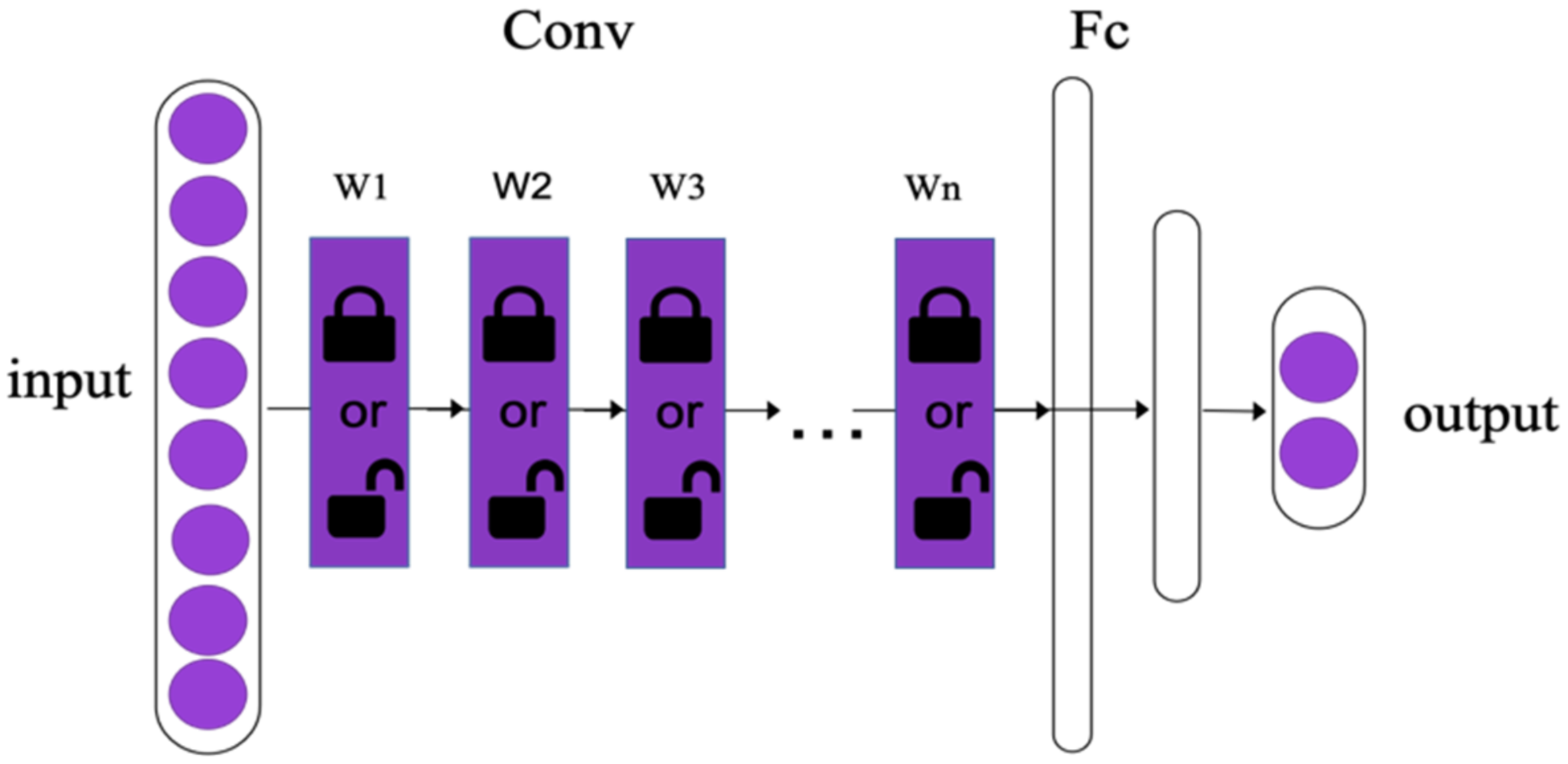
3.4. Transfer-Learning

During this experiment, two fine-tuning strategies were adopted, namely, shallow fine-tuning and deep fine-tuning, as shown in Figure 4. Shallow fine-tuning only trains the fully connected layer, freezing other layer parameters of the network. Deep fine-tuning is to train all layers. The shallow convolution layer extracts basic features of the image, such as edges, contours, etc., the deep convolution layer extracts the abstract features and the connected layer is necessary for classification. The pre-training model used in this article was trained on a large dataset and has basic features and abstract special diagnosis extraction capabilities. For datasets similar to natural images, shallow fine-tuning can reduce training time and avoid overfitting. For datasets that are quite different from natural images, deep fine-tuning is equivalent to providing a better initialization parameter, which is conducive to rapid training convergence and improved accuracy.

ImageNet is an image database which contains a large number of natural pictures. The feature layer of the model, which is trained on the large dataset, has strong generalization ability. The top-ranked models achieved satisfactory results, so pre-trained VGG19, ResNet50, DenseNet121 and InceptionV3 model weights were loaded and two fine-tuning strategies, only fully connected layer training and all-layer training, were applied. Since the fully connected layers of each model have different depth and to better compare the performance of shallow fine-tuning, we generated 3 deep fully connected layers which connected to the convolutional layer of each CNN model. The initial weights of the pre-trained model were loaded into the new model to fine-tune to fit the new task.

3.5. General Configuration

The dataset was obtained via manual collection of laser engraving images captured by metallographic microscope and it included 1986 color images of four different laser carving morphologies. One of the types is defect-free surface, containing 924 pictures. The remainder contains 1062 images of three kinds of laser engraving surface defects. The size of each type of image is 3664 × 2748 pixels. Defect classification is a big challenge because of changes in texture and different sizes, shapes and illumination. We used five-fold cross-validation to evaluate the networks. In the experiment, we popped one subset as the testing dataset and the rest subsets as training dataset and validation dataset, sequentially. All methods were implemented using the Tensorflow 2.0 software and GPU NVIDIA 1080 TITAN with 12 GB memory.

The training of each CNN needs about 10–20 min, which depends on the fine-tuning strategy and training parameters of different models. To find the optimum convergence, we monitored the performance indexes of the training process.

Table 1. Hyperparameters in experiment for fine-tuning.

Hyperparameter	Learning Rate	Decay	Batch Size	Optimizer	Loss
value	0.001	0.9	32	Adam	Binary_crossentropy

presents the settings of the hyperparameters during the experiments.

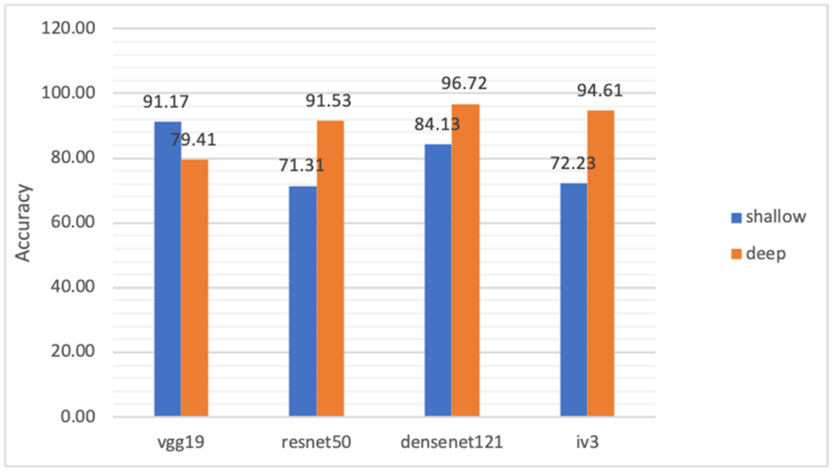
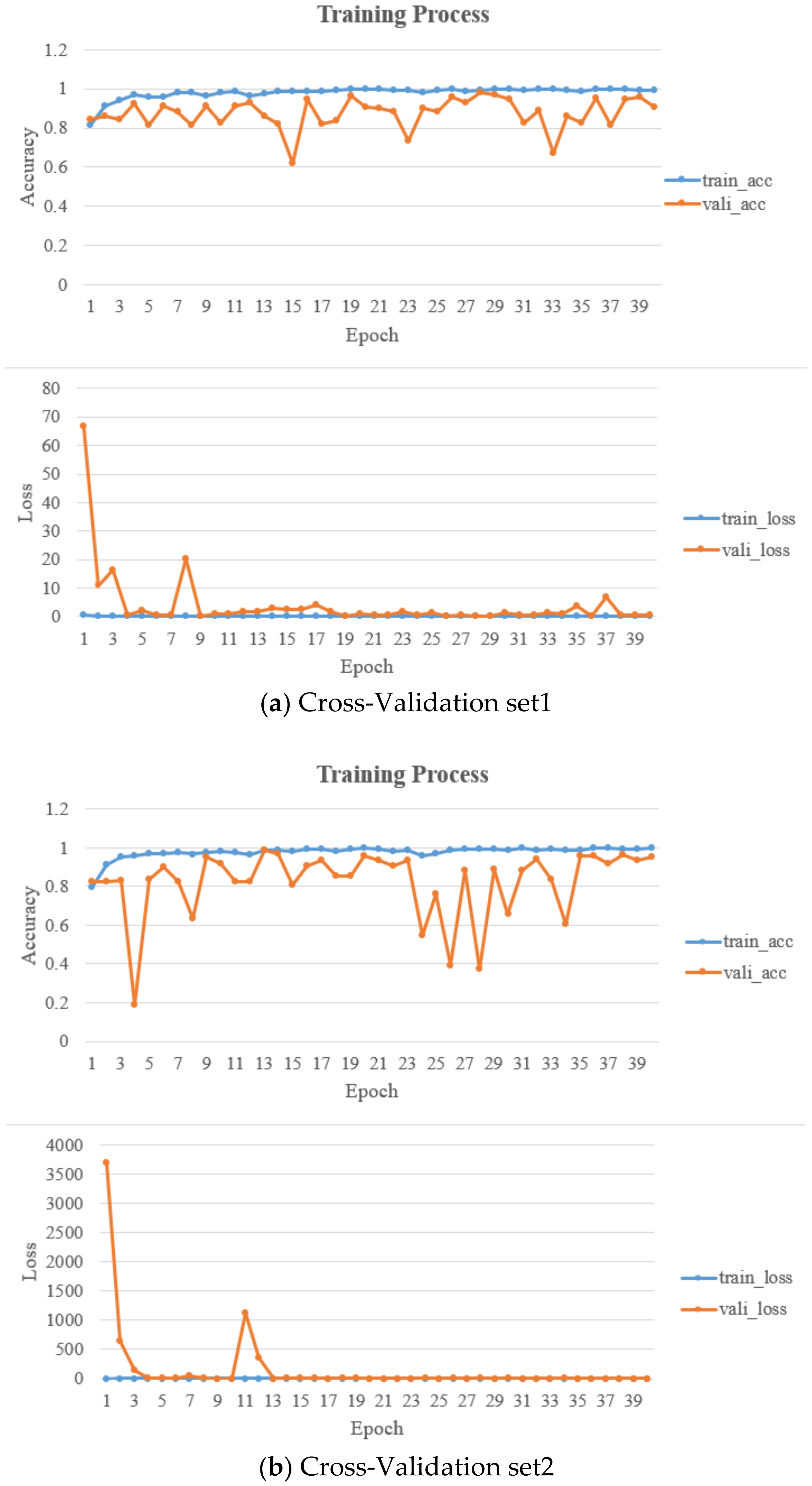
4. Experimental Results and Discussion

In this research, we show a small part of deep transfer learning, which can accurately classify the defects of the engraving topography. The number of collected image datasets was small, so transfer learning was used to train the CNN model.

In order to avoid errors caused by different types of defects in the test set, this paper used a five-fold verification method to evaluate network performance. The data used in this paper were uniformly distributed and the accuracy of the use was determined as the main criterion. In addition, to observe the effect of the model in the f1-score as the true standard sample and the sample as the positive sample, the introduction rate and the reasonable rate were used as evaluation. The f1-score was used as a true standard sample and also used as an evaluation.

Table 2. The classification performance of the proposed method.

Fine-Tuning	Recall	Precision	F1-Score	Accuracy
VGG19 FT, shallow	96.03	83.47	86.53	91.17
VGG19 FT, deep	91.84	72.94	77.83	79.41
ResNet50 FT, shallow	86.32	65.42	68.32	71.31
ResNet50 FT, deep	93.31	88.15	87.12	91.53
DenseNet121 FT, shallow	91.31	82.13	73.14	84.13
DenseNet121 FT, deep	97.15	92.03	91.14	96.72
InceptionV3 FT, shallow	87.42	67.76	83.04	72.23
InceptionV3 FT, deep	92.13	88.56	86.31	94.61

compares the results of the VGG19, ResNet50, DenseNet121 and InceptionV3 networks on the test set using surface fine-tuning and shallow fine-tuning.

The deep fine-tuned DenseNet121 model performed best on the test set and its accuracy and f1-score were 96.72% and 91.14%, respectively. The shallow fine-tuned ResNet50 model performed the worst on the test set and its accuracy and f1-score were 71.31% and 38.32%, respectively. Figure 5 shows the comparison of the accuracy of each model. Figure 6 shows the accuracy and loss for the best performing method. It can be observed from the figures that the best model converges when the epoch is between 20 and 30.

Table 3. Comparison of other classification effects.

Method	Accuracy (%)
LBP + SVM	83.03
GLCM + SVM	78.79
VGG19	91.17
ResNet50	91.53
DenseNet121	96.72
InceptionV3	94.61

compares the detection accuracy of different methods. The accuracy of the GLCM + SVM and LBP + SVM methods based on machine learning on the test set were all worse than those using deep learning. Furthermore, DenseNet121 achieved the highest accuracy of 96.72%, which is much higher than the 83.03% of LBP + SVM.

5. Conclusions

Through a large number of experiments, we demonstrated the application of neural network to accurately classify the defects of laser engraving surfaces based on transfer learning. In addition, we evaluated the classification effects of VGG19, ResNet50, DenseNet121 and InceptionV3 models on transfer learning. The application of transfer learning ResNet50, DenseNet121 and InceptionV3 models improved performance, compared with the method of training-only on the full-connected layer.

Furthermore, the effect of transfer learning was evaluated on VGG19, ResNet50, DenseNet121 and InceptionV3. Thus, the application of th all-layer training fine-tuning method on ResNet50, DenseNet121 and InceptionV3 improved the performance, compared with the method of training-only on fully connected layers.

The size of the dataset is very important for CNN; large-scale data is good for representation learning. However, the images we collected were limited. Therefore, we used the transfer learning technology to train the CNN models. Because of the big differences between images, we did not obtain high accuracy through shallow fine-tuning, which freezes the weights of convolutional layers. As mentioned above, in transfer learning, there should be some similarity between the pre-training dataset and the testing dataset. Our approach shows the transferability of classification in the laser engraving field using the pre-trained models from ImageNet via deep fine-tuning. It is known that the former convolutional layers extract shallow features and the latter layers extract more detailed features. Shallow fine-tuning achieved the best performance because the distributions of the dataset were similar. However, the laser engraving dataset had significant difference, compared to the natural dataset. Thus, we used deep fine-tuning methods to extract features for classification. With the increase in the training layer, complex features of laser engraving images can be learned by CNN models. As shown in Figure 4, deep fine-tuning models achieved better performance, compared with shallow fine-tuning, except VGG19. We assume that the natural images and laser engraving images may have similar distributions in the low-level feature space formed by the pre-trained VGG19.

The focus of current research is on laser engraving surface defect classification for 2D images. As the size of the dataset was limited, we did not train a fresh model from scratch. We adopted four remarkable models, including VGG19, ResNet50, DenseNet121 and InceptionV3, followed by three deep fully connected layers. We trained these models by fine-tuning transfer learning weights. All-layer training of CNNs showed promising performance. Moreover, the pre-trained DenseNet121 is the best model for the classification of laser engraving surfaces. In this paper, due to the huge workload of collecting microscopic laser engraving surface images and labeling, we only performed binary classifications of whether the microscopic images were defective and did not train a multi-classification model to determine which type of defect the defective images have. In future research, we will continue to collect and annotate images and conduct multi-classification model training. At the same time, we will conduct experiments using few-shot learning and active learning technologies to reduce the cost of labeling, while ensuring the accuracy of classification.

References

1. Ebayyeh, A.A.R.M.A.; Mousavi, A. A Review and Analysis of Automatic Optical Inspection and Quality Monitoring Methods in Electronics Industry. IEEE Access 2020, 8, 183192–183271. [Google Scholar] [CrossRef]
2. Wang, M.-J.J.; Huang, C.-L. Evaluating the Eye Fatigue Problem in Wafer Inspection. IEEE Trans. Semicond. Manuf. 2004, 17, 444–447. [Google Scholar] [CrossRef] [Green Version]
3. Jiang, B.C.; Wang, Y.M.W.C.C. Bootstrap sampling technique applied to the PCB golden fingers defect classification study. Int. J. Prod. Res. 2001, 39, 2215–2230. [Google Scholar] [CrossRef]
4. Kim, B.; Jeong, Y.S.; Tong, S.H.; Jeong, M.K. A generalized uncertain decision tree for defect classification of multiple wafer maps. Int. J. Prod. Res. 2020, 58, 2805–2821. [Google Scholar] [CrossRef]
5. Kang, S.; Cho, S.; An, D.; Rim, J. Using Wafer Map Features to Better Predict Die-Level Failures in Final Test. IEEE Trans. Semicond. Manuf. 2015, 28, 431–437. [Google Scholar] [CrossRef]
6. Baly, R.; Hajj, H. Wafer Classification Using Support Vector Machines. IEEE Trans. Semicond. Manuf. 2012, 25, 373–383. [Google Scholar] [CrossRef]
7. Ooi, P.L.; Sok, H.K.; Kuang, Y.C.; Demidenko, S.; Chan, C. Defect cluster recognition system for fabricated semiconductor wafers. Eng. Appl. Artif. Intell. 2013, 26, 1029–1043. [Google Scholar] [CrossRef] [Green Version]
8. Kuo, C.-F.J.; Tung, C.-P.; Weng, W.-H. Applying the support vector machine with optimal parameter design into an automatic inspection system for classifying micro-defects on surfaces of light-emitting diode chips. J. Intell. Manuf. 2016, 34, 123–141. [Google Scholar] [CrossRef]
9. Sun, T.-H.; Tien, F.-C.; Kuo, R.-J. Automated thermal fuse inspection using machine vision and artificial neural networks. J. Intell. Manuf. 2016, 27, 639–651. [Google Scholar] [CrossRef]
10. Chiou, Y.-C.; Lin, C.-S.; Chiou, B.-C. The feature extraction and analysis of flaw detection and classification in BGA gold-plating areas. Expert Syst. Appl. 2008, 35, 1771–1779. [Google Scholar] [CrossRef]
11. Hussain, B.; Jalil, B.; Pascali, M.A.; Imran, M.; Serafino, G.; Moroni, D.; Ghelfi, P. Thermal vulnerability detection in integrated electronic and photonic circuits using infrared thermography. Appl. Opt. 2020, 59, E97–E106. [Google Scholar] [CrossRef]
12. Lu, H.; Mehta, D.; Paradis, O.; Asadizanjani, N.; Tehranipoor, M.; Woodard, D. FICS-PCB: A Multi-Modal Image Dataset for Automated Printed Circuit Board Visual Inspection. IACR Cryptol. ePrint Arch. 2020, 2020, 366. [Google Scholar]
13. Sathiaseelan, M.A.M.; Paradis, O.P.; Taheri, S.S.T.; Asadizanjani, N. Why Is Deep Learning Challenging for Printed Circuit Board (PCB) Component Recognition and How Can We Address It? Cryptography 2021, 5, 9. [Google Scholar] [CrossRef]
14. Senthikumar, M.; Palanisamy, V.; Jaya, J. Metal surface defect detection using iterative thresholding technique. In Proceedings of the Second International Conference on Current Trends in Engineering and Technology—ICCTET, Piscataway, NJ, USA, 8 July 2014; pp. 561–654. [Google Scholar]
15. Wang, C.; Guan, S.; Li, W.; Hong, B.; Liang, H. Surface defect detection method of mechanical parts based on target feature. In Proceedings of the 6th International Conference on Mechatronics, Materials, Biotechnology and Environment (ICMMBE 2016), Yinchuan, China, 13–14 August 2016; pp. 229–232. [Google Scholar]
16. Medina, R.; Gayubo, F.; Gonzalez, L.M.; Olmedo, D.; García-Bermejo, J.G.; Casanova, E.Z.; Per’an, J.R. Surface defects detection on rolled steel strips by Gabor filters. In Proceedings of the Third International Conference on Computer Vision Theory and Applications, Funchal, Portugal, 22–25 January 2008; pp. 479–485. [Google Scholar]
17. Wu, G.; Zhang, H.; Sun, X.; Xu, J.; Xu, K. A brand-new feature extraction method and its application to surface defect recognition of hot rolled strips. In Proceedings of the IEEE International Conference on Automation and Logistics, Jinan, China, 18–21 August 2017; pp. 2069–2074. [Google Scholar]
18. Liu, W.; Yan, Y. Automated surface defect detection for cold-rolled steel strip based on wavelet anisotropic diffusion method. Int. J. Ind. Syst. Eng. 2014, 17, 224–239. [Google Scholar] [CrossRef]
19. Ashour, M.W.; Khalid, F.; Halin, A.A.; Abdullah, L.N.; Darwish, S.H. Surface defects classification of hot-rolled stell strip using multi-directional shearlet features. Arab. J. Sci. Eng. 2019, 44, 2925–2932. [Google Scholar] [CrossRef]
20. Ojala, T.; Pietikinen, M.; Menp, T. Gray Scale and Rotation Invariant Texture Classification with Local Binary Patterns; Springer: Berlin/Heidelberg, Germany, 2000; Volume 44, pp. 341–350. [Google Scholar]
21. Chen, P.H.; Lin, C.J.; Schölkopf, B. A tutorial on ν-support vector machines. Appl. Stoch. Models Bus. Ind. 2005, 21, 111–136. [Google Scholar] [CrossRef]
22. Yang, B.-B.; Shen, S.-Q.; Gao, W. Weighted Oblique Decision Trees. Proc. Conf. AAAI Artif. Intell. 2019, 33, 5621–5627. [Google Scholar] [CrossRef] [Green Version]
23. Yuk, E.H.; Park, S.H.; Park, C.-S.; Baek, J.-G. Feature-Learning-Based Printed Circuit Board Inspection via Speeded-Up Robust Features and Random Forest. Appl. Sci. 2018, 8, 932. [Google Scholar] [CrossRef] [Green Version]
24. Boser, B.E.; Guyon, I.M.; Vapnik, V.N. A training algorithm for optimal margin classifiers. In Proceedings of the Fifth Annual ACM Workshop on Computational Learning Theory, Pittsburgh, PA, USA, 27–29 July 1992; pp. 144–152. [Google Scholar]
25. Sindagi, V.A.; Srivastava, S. Domain Adaptation for Automatic OLED Panel Defect Detection Using Adaptive Support Vector Data Description. Int. J. Comput. Vis. 2017, 122, 193–211. [Google Scholar] [CrossRef]
26. Li, T.-S.; Huang, C.-L. Defect spatial pattern recognition using a hybrid SOM–SVM approach in semiconductor manufacturing. Expert Syst. Appl. 2009, 36, 374–385. [Google Scholar] [CrossRef]
27. Liao, C.-S.; Hsieh, T.-J.; Huang, Y.-S.; Chien, C.-F. Similarity searching for defective wafer bin maps in semiconductor manufacturing. IEEE Trans. Autom. Sci. Eng. 2014, 11, 953–960. [Google Scholar] [CrossRef]
28. Cha, Y.-J.; Choi, W.; Büyüköztürk, O. Deep Learning-Based Crack Damage Detection Using Convolutional Neural Networks. Comput. Aided Civ. Infrastruct. Eng. 2017, 32, 361–378. [Google Scholar] [CrossRef]
29. Kuo, F.-J.; Hsu, C.-T.-M.; Liu, Z.-X.; Wu, H.-C. Automatic inspection system of LED chip using two-stages back-propagation neural network. J. Intell. Manuf. 2014, 25, 1235–1243. [Google Scholar] [CrossRef]
30. Su, C.-T.; Yang, T.; Ke, C.-M. A neural-network approach for semiconductor wafer post-sawing inspection. IEEE Trans. Semicond. Manuf. 2002, 15, 260–266. [Google Scholar] [CrossRef]
31. Azizpour, H.; Razavian, A.S.; Sullivan, J.; Maki, A.; Carlsson, S. From generic to specific deep representations for visual recognition. arXiv 2014, arXiv:1406.5774. [Google Scholar]
32. Bar, Y.; Diamant, I.; Wolf, L.; Greenspan, H. Deep Learning with Non-Medical Training Used for Chest Pathology Identification. In Medical Imaging 2015: Computer-Aided Diagnosis; International Society for Optics and Photonics (SPIE): Bellingham, WA, USA, 2015; Volume 9414, p. 94140V. [Google Scholar]
33. Huang, G.-B.; Zhou, H.; Ding, X.; Zhang, R. Extreme Learning Machine for Regression and Multiclass Classification. IEEE Trans. Syst. Man Cybern. Part B Cybern. 2012, 42, 513–529. [Google Scholar] [CrossRef] [PubMed] [Green Version]
34. Huang, G.B.; Zhu, Q.Y.; Siew, C.K. Extreme Learning Machine: A New Learning Scheme of Feedforward Neural Networks. In Proceedings of the 2004 IEEE International Joint Conference on Neural Networks, Budapest, Hungary, 25–29 July 2004; Volume 2, pp. 985–990. [Google Scholar]
35. Huang, G.-B. Can threshold networks be trained directly? IEEE Trans. Circuits Syst. II Express Briefs 2006, 53, 187–191. [Google Scholar] [CrossRef]
36. Huang, G.-B.; Zhu, Q.-Y.; Siew, C.-K. Real-Time Learning Capability of Neural Networks. IEEE Trans. Neural Netw. 2006, 17, 863–878. [Google Scholar] [CrossRef] [Green Version]
37. Yang, H.; Mei, S.; Song, K.; Tao, B.; Yin, Z. Transfer-Learning-Based Online Mura Defect Classification. IEEE Trans. Semicond. Manuf. 2018, 31, 116–123. [Google Scholar] [CrossRef]
38. Imoto, K.; Nakai, T.; Ike, T.; Haruki, K.; Sato, Y. A CNN-Based Transfer Learning Method for Defect Classification in Semiconductor Manufacturing. IEEE Trans. Semicond. Manuf. 2019, 32, 455–459. [Google Scholar] [CrossRef]
39. Simonyan, K.; Zisserman, A. Very deep convolutional networks for large-scale image recognition. In Proceedings of the 3rd International Conference on Learning Representations (ICLR 2015), San Diego, CA, USA, 7–9 May 2015; pp. 1–14. [Google Scholar]
40. He, K.; Zhang, X.; Ren, S.; Sun, J. Deep Residual Learning for Image Recognition. In Proceedings of the 2016 IEEE Conference on Computer Vision and Pattern Recognition (CVPR), Las Vegas, NV, USA, 27–30 June 2016; pp. 770–778. [Google Scholar]
41. Huang, G.; Liu, Z.; Van Der Maaten, L.; Weinberger, K.Q. Densely Connected Convolutional Networks. In Proceedings of the 30th IEEE Conference on Computer Vision and Pattern Recognition (CVPR), Honolulu, HI, USA, 21–26 July 2017; pp. 2261–2269. [Google Scholar] [CrossRef] [Green Version]
42. Szegedy, C.; Vanhoucke, V.; Ioffe, S.; Shlens, J.; Wojna, Z. Rethinking the Inception Architecture for Computer Vision. In Proceedings of the IEEE Computer Society Conference on Computer Vision and Pattern Recognition, Las Vegas, NV, USA, 26 June–1 July 2016; pp. 2818–2826. [Google Scholar] [CrossRef] [Green Version]
Figure 1. Design of method.
Electronics 10 01993 g001
Figure 2. Label of carving position on the mobile phone shell.
Electronics 10 01993 g002
Figure 3. Types of laser engraving defects. (a) Defect-free surface; (b) defect surface.
Electronics 10 01993 g003
Figure 4. Shallow and deep fine-tuning.
Electronics 10 01993 g004
Figure 5. Accuracy performance comparison of two fine-tuning strategies on different pre-trained CNN models.
Electronics 10 01993 g005
Figure 6. Training process. The accuracy and loss history of the best model, training-all densenet121. (ae) represent the effect of each set.
Electronics 10 01993 g006aElectronics 10 01993 g006bElectronics 10 01993 g006c