Abstract
In industrial production planning problems, the accuracy of the accessible market information has the highest priority, as it is directly associated with the reliability of decisions and affects the efficiency and effectiveness of manufacturing. However, during a collaborative task, certain private information regarding the participants might be unknown to the regulator, and the production planning decisions thus become biased or even inaccurate due to the lack of full information. To improve the production performance in this specific case, this paper combines the techniques of machine learning and model predictive control (MPC) to create a comprehensive algorithm with low complexity. We collect the historical data of the decision-making process while the participants make their individual decisions with a certain degree of bias and analyze the collected data using machine learning to estimate the unknown parameter values by solving a regression problem. Based on an accurate estimate, MPC helps the regulator to make optimal decisions, maximizing the overall net profit of a given collaborative task over a future time period. A simulation-based case study is conducted to validate the performance of the proposed algorithm in terms of estimation accuracy. Comparisons with individual and pure MPC decisions are also made to verify its advantages in terms of increasing profit.
1. Introduction
In modern industry, the participants of a manufacturing task usually work in a collaborative mode, which substantially increases productivity [1]. The individual decisions of the participants contribute to changes in state variables within the industrial process, which in turn affect their own task performance. To address this decision-making process, a dynamic model of the given collaborative task is established to represent the interaction and communication between the participants [2]. Within these collaborative tasks, each participant naturally makes individual decision to optimize their own task performance, if no decision is made by the regulator. However, the optimal decisions for the overall optimal task performance usually conflict with these individual decisions according to the Nash Equilibrium [3]. Furthermore, the participants might even make individual decisions with a certain bias and fail to optimize their individual benefits due to a lack of professional experience. Therefore, an essential responsibility for regulators is to optimize the overall task performance rather than any individual’s performance, which creates production planning problems in a collaborative mode.
The class of production planning problems aims at making appropriate decisions for an industrial manufacturing process to optimize the performance of certain tasks and yield various practical benefits, such as maximum net profits [4,5,6], fuzzy multiple objectives [7,8,9], economic production quantity [10] and optimal emission policy [11,12]; see [13,14,15,16,17] for detailed overviews of production planning problems. Most existing production planning methods assume that all information within their problem formulations are known as a priori. Nevertheless, this paper focuses on the production planning problems in collaborative tasks, which contain private information regarding participants that might be unknown to the regulator. In this sense, the regulator cannot obtain the full scope of accurate market information to make optimal decisions for participants, which is an obstacle to making reliable decisions.
To accurately estimate the parameter values of unknown private information, the data-driven technique of machine learning is considered in this paper, which is a collection of approaches for making inferences based upon historical data [18]. This approach extracts useful information from a realistic data set to tune the weighting parameters of a trained model, meaning that this model asymptotically returns desired information to the users [19]. This advantage unlocks intelligent solutions to certain design problems that can hardly be characterized using classical methods due to their complexity and fuzziness [20]. Numerous machine learning procedures have been proposed in different research areas, such as image classification [21,22], data classification and clustering [23,24,25], system identification [26], natural language processing [27], autonomous driving [28] and fault diagnosis [29,30]. Most of these state-of-the-art machine learning approaches are designed for classification tasks with various data types, such as images, audio and video. However, this paper addresses a parameter estimation task by solving a regression problem based on the recorded biased individual decisions, and a “gradient descent”-based machine learning pipeline is proposed to fulfill this task in an efficient manner.
The technique of MPC is employed in this paper to solve the specific production planning problem based on the estimated parameter values. We generally exploit the model and current state information to predict future information so that an appropriate decision is made to optimize the overall task performance over a future time period, which is computationally efficient [31]. Because of this key feature, various MPC methods have been implemented to improve the task performance of broad applications, such as sludge processes [32], micro-grid [33] and power electronics [34]; see [35,36,37] for more details about MPC. Although some existing works in the literature—e.g., [38,39,40]—handle the production planning problem with uncertain variables, their problem formulations were different from that discussed in this paper with disembedded machine learning or MPC methods. Moreover, this machine learning-based MPC method is capable of extracting the target information from a complex but real historical data set and carrying out the estimation procedure in an off-line fashion. It outperforms other on-line learning based MPC methods—e.g., [41,42,43,44]—in terms of its small computation load.
To overcome the aforementioned problems, this paper combines the techniques of machine learning and MPC to aid regulators to compute optimal decisions for the participants, solving the production planning problem with a maximum overall net profit. Note that some preliminary results of this paper have been reported in [45], but significant extensions are proposed in this paper. A detailed discussion is made of technical issues such as Remarks 1–4, an entirely new section (Section 4, Implementation Instructions) is added to help the reader to understand the behind-screen parameter tuning mechanism of the algorithm, the case study section employs a newly established model to handle the problem, and the results have been improved compared to those in the published paper because of the new contributions added in this paper. The contributions of this paper are highlighted as follows:
- The production planning problem is formulated using a discrete time system, with task performance judged by net profit;
- A gradient descent machine learning procedure with an adaptive learning scheme is developed to estimate the unknown parameters of the revenue in Q using historical data via solving a regression problem;
- An MPC method uses the estimated values of Q as its user-defined weight factors to predict the optimal decisions to maximize net profit;
- A machine learning-based MPC algorithm with low complexity is proposed and validated in a simulation-based case study;
- A comparison with individual and pure MPC decisions is performed to show the increase in profit.
The nomenclature is listed as follows:
| is an n-dimensional Euclidean vector space, | |
| is an real matrix space, | |
| is the element in ith row and jth column of A, | |
| is a diagonal matrix of its argument, | |
| is the spectral radius of a given matrix, | |
| is an input constraint set, | |
| is a cost function of the performance index, | |
| is the infinity norm of the vector x, | |
| is the projection of x onto the set , | |
| is the representation of normal distribution, | |
| is the estimated value of x, | |
| is a loss function, | |
| is the set of integer numbers, | |
| is the set of non-negative integer numbers, | |
| s | is the production demand, |
| Q | is the weighting parameters of the revenue, |
| R | is the weighting parameters of the productivity effort, |
| P | is the decision bias parameters of the participants, |
| is the benchmark of the unknown parameters. |
2. Problem Formulation
This section introduces the system dynamics and uses certain cost functions to represent the desired task performance. Then, the production planning problem with a collaborative mode and unknown information is formulated, and the effect of unknown parameters is discussed.
2.1. System Dynamics
In this paper, the interaction among participants within a given collaborative manufacturing task is modeled by a discrete time system with the following state space representation:
The system input and the system state denote the productivity decisions and market sizes of all n participants at sample time index k, respectively. The matrices A and B are of compatible dimensions; i.e., .
The future state of the discrete time system (1) is triggered by the current state and the current input . In other words, the market size of each participant at the next sample time depends on the current market sizes of the participants as well as the current productivity decision. Therefore, the individual decision of each participant influences the market sizes of others, and their market size is also affected by the individual decisions of others, which gives rise to the system dynamics. If , the discrete time system (1) is stable. The matrix B is diagonal, i.e.,
as the decision of an individual participant does not directly affect the market sizes of other participants, and its diagonal elements are non-negative since the productivity clearly has a positive relationship with respect to the market size.
Remark 1.
The problem formulation in this paper can be naturally extended to other non-linear systems without difficulties. However, this kind of extension requires extra modifications to the solution to the production planning problem, which is not discussed in this paper.
2.2. System Constraints
In practice, it should be realized that the system variables have specific physical limits that give rise to different forms of system constraints. For example, the system input
represents the productivity of the participants at sample time index k, and all its elements , must be non-negative and have an upper bound for maximum productivity. The input constraint set usually represents the acceptable system input range. In this paper, the input saturation constraint , i.e.,
is considered and used to compute the solutions of the production planning problem in latter sections, where denotes the input upper bound.
2.3. Production Planning Design Objectives
In a manufacturing task, the overall task performance is generally represented by a cost function consisting of the productivity decision u, the market size x and the sample time index k. For example, the change in market size is denoted as
and the maximum productivity is denoted as
Note that the cost function does not necessarily need to incorporate all variables of u, x and k, and its exact definition can change in terms of the target performance index to be optimized. To improve the task performance, the regulator should make an appropriate decision for the participants to optimize a certain performance index. This design objective brings significant practical benefits within the given task. Therefore, the production planning problem explored in this paper is formulated in the following definition.
Definition 1.
TheProduction Planning Problemrefers to the choice of an appropriate productivity decision of a discrete time system (1) at sample time index k, such that the desired cost function is optimized over the time period ; i.e.,
To exemplify this design objective, this paper takes the overall net production profit of a collaborative manufacturing task to be the task performance, defined as
where and are the revenue function and the effort function with respect to the sample time index k. This cost function makes sense in practice as the production effort made at sample time index brings the revenue in the next sample time index k.
The revenue function is in a quadratic form,
where the diagonal matrix
contains the constant weighting parameters of the revenue for each participant, and the vector
represents the production demands of the participants at sample time index k, which is a known time-varying value. In the problem formulation, the production demand is the required order number of the products and does not have a direct relationship with the market size , which denotes the actual number of products made by the factory. However, they together contribute to the revenue function . According to the quadratic form (9), the revenue of each participant first increases to a peak value and then decreases along its market size axis. Due to the fact of excess demand, the overall revenue decreases after a certain market size. Note that the revenue is zero for zero market size, which is realistic in practice. The production demand is not a fixed value as the demand for certain products may vary with respect to the sample time index k. In addition, the production demand has a positive effect on the revenue, as an increase of production demand increases the product price.
The effort function is in a quadratic form,
where the diagonal matrix
contains the constant weighting parameters of the productivity effort for the participants. Based on the quadratic form (12), the effort of each participant increases quadratically as its productivity increases from the value of zero. This quadratic form is realistic as high productivity generally leads to extra costs in terms of human power, machine damage and energy consumption.
To solve the production planning problem (7), a reliable system model (1) and accurate values of R, Q and are required. However, unknown parameters occur frequently in the practical production planning problem. In this specific case, the participators naturally attempt to optimize their private performance index, and their individual decisions might even conflict with the optimal decisions made by the regulator for the overall task performance. Therefore, they might not share their private revenue weighting parameters with the regulator or provide inaccurate values. Thus, the matrix Q is generally unknown or inaccurate to the regulator, which restricts the reliability of optimal decisions.
To handle this problem, the data-driven method of machine learning is applied to estimate these unknown parameters by extracting and analyzing the information from the recorded historical data, and MPC is then used to provide optimal decisions for the regulator based on estimated parameter values.
3. Machine Learning-Based MPC
In this section, a formula is derived to model the individual decisions of the participants under the free decision making condition. A gradient descent machine learning training procedure with low complexity is proposed to estimate the unknown parameters using the recorded historical data and the obtained formula. Then, MPC is considered to solve the problem (7) based on the estimated values of the parameters to yield the optimal decisions.
3.1. Individual Decision Modeling
A free decision making condition is now supposed for the participators, meaning that there are no optimal decisions received from the regulator. Therefore, they have the authorization to make individual decisions for themselves. It is not surprising that the individual decisions are often biased from their optimal value due to the low response to market environment change and the restricted insight of the participators. In this sense, the decision bias matrix
is introduced to provide the decision bias parameters of the participants. These parameters , are unknown random values with a normal distribution , where is the mean value and is the standard deviation. The decision bias parameters represent the inherent difference between actual individual decisions and associated optimal options. By introducing these parameters, a representation formula of the individual decisions is derived and shown in the next theorem.
Theorem 1.
Under the free decision making condition, the participant attempts to maximize their individual task performance, defined by the cost function
at sample time index k, and the individual decision is
where involves the unknown parameters of the participant and function is defined by
with the projection operator
Proof.
Under the free decision making condition, each participant makes their decision actively and focuses on maximizing their individual cost function (15), which gives rise to
The problem (19) is a quadratic programming problem, and the partial differentiation of the cost function is performed with respect to to find the identical stationary point. As the problem is convex, this stationary point is the global minimum and gives the unconstrained solution
Using the decision bias parameter , the actual decision of each participant is
To satisfy the input constraint, the projection operator is used to provide the individual decision (16). □
The above theorem derives a representation formula of the individual decisions under the free decision making condition. It not only attempts to optimize the individual task performance of each participant but also incorporates the decision bias into the individual decision making processes. Moreover, the representation formula of the individual decision vector is stated in the next corollary.
Corollary 1.
According to the Formula (16) in Theorem 1, the overall individual decisions are equivalently written into the vector form
where denotes the benchmark of the unknown parameters and function is defined by
with the projection operator
3.2. Gradient Descent Machine Learning
In industry, it is normal practice to record historical production information. Suppose that the historical data are recorded over m sample times under the free decision making condition, and the data set with m elements is generated and stored. Each element contains the decision, the state and the production demand, which are linked by the function as
according to Corollary 1. However, is unknown in the general sense, and the estimate is employed in this paper to denote all unknown parameters within the function . In this sense, an accurate estimate definitely provides a decision x), which approaches the real value u. This fact motivates the data-driven technique of machine learning to estimate the benchmark . The machine learning problem and its design objective are stated in the following definition.
Definition 2.
Themachine learning problemaims at iteratively updating the estimate such that the decision loss function
is minimized for all .
In the above problem definition, the decision loss denotes the difference between the decision computed from the estimate and the recorded historical decision u. If the decision loss is sufficiently small, the estimated decision approximates u and the estimate is considered as an approximation of the benchmark . Once an accurate estimate is available, more reliable model information becomes possible for the later MPC procedure as it considers the values of while solving the optimization problem.
Furthermore, the decision loss function of each participant is defined as
the sum of which gives rise to the overall decision loss function; i.e.,
The widely used method of machine learning is an iterative training procedure with several training epochs and an initial estimate
This method randomly splits a total number of elements from the data set into a training set , and the rest are sorted into a testing set [46]. At each training epoch, it updates the estimate using each element in the training set to reduce the decision loss (26). At the end of each training epoch, the decision loss (26) of the elements in the testing set , i.e.,
is computed to evaluate the training performance of the machine learning method; in other words, the decision loss, where the subscript denotes the training epoch number. Since the testing set is independent of the training set , it is possible to use the evaluation results to double-check the training performance of the machine learning design using external data from the training set, which avoids the limitation of over-fitting.
A gradient descent machine learning training procedure is proposed to reduce the decision loss (26) with respect to the elements in the training set during each training epoch. The training procedure of each training element is illustrated in the following theorem:
Theorem 2.
For , the estimate is updated by using the gradient descent update
such that the overall decision loss is reduced; i.e.,
where and are partial derivatives of (26) with respect to and , and is the adaptive learning rate defined by
where and are constant scalars, and is the smallest non-negative integer such that
Proof.
This gradient descent machine learning training procedure aims at updating the estimate to reduce the decision loss of all elements in the training set and obtains a reliable estimate of the unknown parameter values after sufficient training epochs.
Remark 2.
K-fold cross-validation is recommended if the amount of historical data is relatively small. Different splits of the data enable the cross validation using all elements within the historical data set [47]. The adaptive learning rate choice (33) is a mechanism used to ensure both the maximum gradient descent step size and the reduction of the decision loss. Other alternative learning rate choices can be made using bisection or back-stepping methods.
Remark 3.
For each element , there exist infinite choices for to reduce its decision loss to zero, but there only exists a rather small range for in the search space to obtain a sufficiently small overall decision loss. The trial and error method is used in (31) to reduce the decision loss of all in a random order, with the aim of minimizing the overall decision loss. However, its convergence performance along with the training number cannot always be guaranteed due to the independence of the elements in Λ; i.e., an update of may reduce but increase .
Remark 4.
Note that other non-iterative methods, such as echo-state networks, extreme learning machines or kernel ridge regression, are also capable of solving the regression design objective shown in Definition 2.
Remark 5.
In more general production planning problem, due to different system dynamics, the function may become complex/fuzzy. To handle the machine learning problem, the deep neural network model is suggested to be utilized to estimate the unknown values.
3.3. MPC Production Planning Problem
The machine learning procedure in Section 3.2 is capable of determining the unknown parameter values for the production planning problem. Therefore, an analytic representation of the problem formulation becomes available, and the regulator can make the optimal decisions for the participants to improve the overall task performance. To solve the production planning problem, the technique of MPC is applied at each sample time index k to update the optimal decisions over a future time interval by solving the optimization problem
where is the predicted state at sample time index based on the real information at k and the planned input over the period . At each sample time, MPC uses the current input , the current state and the system dynamics to predict the future states , , over the prediction time period . An appropriate solution is chosen to optimize the cost function consisting of these predicted values and replace the previous decision (if it exists) with this new decision along with the future time period.
The optimal decisions aim at maximizing the overall net profit of the collaborative manufacturing task, while the individual decisions focus on the net profit of an individual participant. A comparison between these decisions is made in Section 5 via a case study, and the benefits of using the optimal decisions are illustrated in details.
4. Implementation Instructions
The instructions are provided in this section for implementing the solutions in Section 3, and a comprehensive algorithm is then proposed to provide a solution to the production planning problem with a collaborative mode and unknown information.
4.1. Instructions on Projection Solution
According to the definition (22) of the projection operator , the unconstrained decision is projected into the given decision constraint set , which generates the constrained decision. The decision saturation constraint (4) is element-wise and the constraint handling procedure is straightforward. The next proposition provides the analytic solution of the projection operator with respect to the decision saturation constraint (4) as an example.
Proposition 1.
Proof.
The above proposition provides the analytic solution of based on the input saturation constraint (4). The solutions of the projection operator with other types of input constraints can be handled in a similar way.
4.2. Instructions on Initial Estimate Choice
The machine learning training procedure is carried out in an iterative manner, and the decision loss function in (26) is generally non-linear and non-convex. Although the gradient descent training procedure (31) guarantees the reduction of the decision loss for the various possible initial estimate choices , the initial estimate choice definitely affects the training performance. The estimate might converge to a local minimum point with a relatively large decision loss if the initial estimate is not chosen properly.
To achieve the desired training performance, the estimate search space is predefined as
where the scalars , , and , , are appropriately chosen as the upper and lower bounds of the search space. In this sense, two different initial estimate choices are introduced, and the first one is defined by
Definition 3.
Thecentral initial estimate choiceis used to specify all initial values as the central values of their intervals; i.e.,
This choice ensures the initial distance to the benchmark does not appear to be too large and provides a relatively fair initial choice. Alternatively, the second choice is defined by
Definition 4.
Thegrid initial estimate choiceis used to specify the initial estimate choice as the best fitting solution to the grid search problem
where is a discretized finite subset of Θ defined by
with sample numbers and .
This word “grid” in the name of this choice implies that the sample numbers and should not be too large so that the total number of elements in would not be excessive [48]. Therefore, the grid search problem (40) can be computed efficiently, capturing an approximate region of the global optimal solution to the minimum decision loss problem:
However, this choice requires extra computational time to carry out the grid search as the number of the unknown parameters increases.
Remark 6.
These two initial choices both provide reliable initial values for the estimate for the gradient descent training procedure (31). However, a trade-off between computational efficiency and training performance improvement should be taken into account for practical implementation.
4.3. Instructions for Partial Derivative Estimation
Since the decision loss function has an analytic form (26), the value of its partial derivatives with respect to and can be computed using the syntax gradient in Matlab or autograd in Python. Alternatively, a numerical estimation
is used to obtain the partial derivative, where
and the scalar is sufficiently small. The partial derivative can be obtained in a similar way. This numerical estimation incurs less computational load and is still capable of giving approximate values of the derivatives even if the analytic representation of the decision loss function is not available in some extreme cases.
4.4. Instructions for MPC Problem Solution
The MPC problem (35) has a quadratic cost function, linear equality constraint and convex inequality constraint. Therefore, it is a quadratic programming problem, which is a convex optimization problem with a global optimal solution. There exist various standard solvers for quadratic programming problems, such as the solver quadprog in MATLAB. These standard solvers can directly provide the global optimal solution.
Furthermore, an alternative computational efficient solution is obtained by decoupling the input constraint from the optimization problem (35) and setting the prediction interval to a unit sample time; i.e., . The solution to the problem (35) is described as first solving the unconstrained problem
and projecting the solution into the input constraint set using , which is illustrated as follows:
Proposition 2.
Proof.
As the input constraint is decoupled and , the problem (35) collapses to the problem (44). The problem (44) becomes an unconstrained problem by substituting the equality constraint into the cost function, which yields the solution (46). To handle the input constraint, the projection operator is considered to give the solution (46). □
The alternative solution to problem (35) in Proposition 2 is computationally more efficient than the direct solution provided by the standard solvers. A trade-off between efficiency and accuracy should be considered by the production regulator according to the properties of the exact production planning scenario.
4.5. Production Planning Comprehensive Algorithm
The techniques of machine learning and MPC are combined to yield a comprehensive algorithm (Algorithm 1) to solve the production planning problem with a collaborative mode and unknown information. This algorithm first uses the gradient descent machine learning procedure to estimate the unknown parameters and applies MPC to obtain the optimal decisions for the participants at each sample time index k. Note that the scalar value N denotes the total number of sample times and is a small scalar depending on the accuracy requirement of machine learning estimation. For a straightforward view, a block diagram of the machine learning-based MPC algorithm is shown in Figure 1.
| Algorithm 1 Machine learning based MPC |
| Input: System dynamics (1), cost function , production demand , initial state , initial estimate , decision loss function and historical data set . |
| Output: Estimate , optimal decision . |
| 1: initialization: Set training epoch number , sample time index and randomly split elements of the set to a training set and the rest to a testing set . |
| 2: while not do |
| 3: Perform the training procedure (31) to update the estimate using all elements in . |
| 4: Perform the evaluation (30) to compute the decision loss , using all elements in . |
| 5: Set to the next training epoch. |
| 6: end while |
| 7: Set the estimate as the unknown matrix Q. |
| 8: while do |
| 9: Solve the MPC problem (35) to obtain . |
| 10: Record the optimal decisions . |
| 11: Set to the next sample time index. |
| 12: end while |
| 13: return , , |
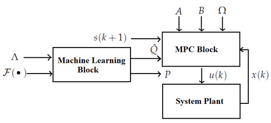
Figure 1.
Block diagram of the machine learning-based MPC algorithm.
5. Simulation-Based Case Study
In this section, a case study of a production planning problem is presented, and an evaluation is conducted to check the performance of Algorithm 1 in comparison to the performance under the conditions of individual decision making and pure MPC decision making.
5.1. Problem Design Specifications
In this paper, we consider the production planning scenario within a clothing factory as a case study. This factory has a total number of 10 departments (; i.e., 10 participant) working in a collaborative mode. The modified dynamics of the discrete time system (1) of this factory are considered with
The above system dynamics demonstrate how the productivity decision of an identical participant affects the market size of other participants. The sample time period is one day, which means the regulator needs to plan productivity decisions one day in advance. The total number of sample times N is 365; i.e., one year. The initial state value is chosen as , and the input saturation constraint (4) is considered with as the productivity of the participants with a maximum load. The benchmark values of matrices R and Q are listed as
The individual decision bias parameters , in matrix P are defined with mean values
as well as a standard deviation of . Since the parameters in the matrix Q are unknown to the regulator, the authors only apply these values as a benchmark to generate historical data and evaluate the estimation accuracy of the machine learning procedure. The same argument holds for the unknown matrix P.
In addition, the production demand of each department over the total decision making period is described as
where the amplitude , center amplitude and the phase are the elements of the vectors as follows:
This case study focuses on clothing manufacturing, so the production demand varies for different seasons in a calendar year. In this sense, the sinusoidal function (47) can reasonably represent the production demands of these departments. These seasonally varying demands contribute to the historical demand within the set and are used to compute the optimal decisions in Section 5.2 and Section 5.3.
These problem design specifications fully replicate the industrial environment of cloth manufacturing. Therefore, the simulation results are capable of indicating the practical effectiveness and feasibility of the proposed algorithm.
5.2. Parameter Estimation Using Machine Learning
To obtain the historical data, the following data sampling procedure was employed: first of all, the benchmark matrices Q and P defined in Section 5.1 generated the individual decisions using the Formula (22) over a production planning period , denoting a calendar year. Therefore, the historical data set was established with a total number of 365 groups of historical data; i.e., , (). In this case study, the groups of data generated as above replicated the interaction between the production demands, individual decisions and market sizes of each department under the free decision making condition and were thus regarded as effective historical data for the later machine learning procedure.
The machine learning procedure of Algorithm 1 randomly split a total number of 100 () groups of the historical data into a training set and the rest into a testing set . Then, it was capable of estimating the unknown parameter values of Q and P based on the obtained training set . The grid initial estimate choice in Definition 4 was carried out in the search space (38) defined by
for . The values and were used to determine the adaptive learning rate choice (33).
The decision loss during the training procedure was plotted along the training number line for each department in Figure 2 and all asymptotically converged to sufficiently small values. Meanwhile, the decision loss of each department was computed using the testing data at the end of each training epoch and plotted as the colored lines in Figure 3. Note that all lines in this figure also asymptotically converged to sufficiently small values. This means that the estimated decision gradually approached the real decision u, and thus the training procedure succeeded in providing an appropriate estimate . The above evaluation demonstrates the feasibility and reliability of the machine learning procedure in terms of validation using testing data. The choice of the initial estimate affected the convergence performance of the 10 departments. For instance, the estimated values of the fourth department were sufficiently close to the benchmark values, and the convergence rate was much slower along the training epochs in comparison to others.
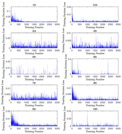
Figure 2.
The decision loss with respect to each group of training data along the training number line for each department.
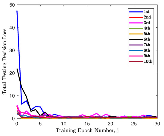
Figure 3.
The decision loss of the testing data at the end of each machine learning training epoch for each department.
Furthermore, the updated estimate was compared with the benchmark values for each training update, and the results of the first department are plotted in Figure 4. For comparison, the corresponding benchmark values are plotted in the same figure as the dashed magenta lines (the mean value of is used for comparison). It is observed that the estimated values asymptotically converged to their benchmark values, which means that the converged estimate matched well with its benchmark. The converged estimates were
which approached the benchmark values shown in Section 5.1. Therefore, the above results reveal the effectiveness of the machine learning procedure for estimating the unknown parameters. The estimated convergence performances of other departments were similar to those in Figure 4 and are thus omitted here for brevity.
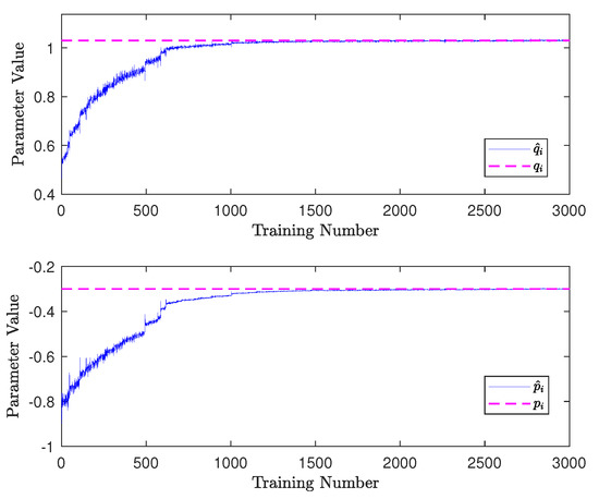
Figure 4.
The comparison between the estimates and the benchmark values along the training number line for the first department.
In practice, the historical data of the production information should be recorded over a past time period rather than artificially generated using the benchmark, as in this case study. The performance of the machine learning procedure should be evaluated based on the convergence performance of the decision loss with respect to the testing data.
5.3. Decision Making Using MPC
Since the machine learning procedure in Section 5.2 provided an accurate estimate of the unknown parameter values, the information within the production problem made it feasible for the regulator to make the optimal decisions. The MPC decision making procedure of Algorithm 1 was performed for the production planning problem specified in Section 5.1 with a unit prediction interval (), using the given system dynamics (1) and the desired cost function (8).
The performance of the MPC decision making procedure was evaluated over the whole production planning period , and the overall net profits of the factory at each sample time index are plotted as the magenta curve in Figure 5. Note that the profit in winter was approximately higher than that in summer. The net profit caused by the individual decisions was computed for the same production planning problem, and the pure MPC approach was utilized for this problem with an inaccurate estimate of a random variance to the benchmark values. These results are also plotted in this figure as the blue and red curves, respectively. These results suggest that the machine learning (ML)-based MPC decisions are able to increase the profit by over compared to the profit of the individual biased decisions. In comparison to the pure MPC decisions, it fully employs the technique of machine learning to obtain an accurate estimate of unknown parameters, increasing the annual profit by around .
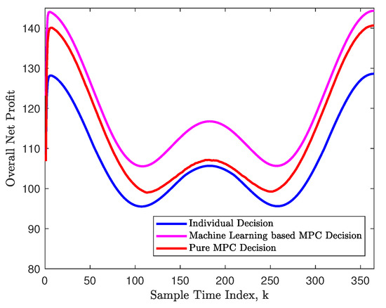
Figure 5.
The comparison of the overall net profits at each sample time index for individual decisions, machine learning-based MPC decision and pure MPC decision.
Furthermore, the optimal decisions of each department are plotted as the colored curves in Figure 6. Note that the optimal decisions were all within the saturation range , which means that Algorithm 1 could handle the input constraint appropriately. Furthermore, the optimal decisions had a causal relationship with the production demand (47). In other words, a higher production demand encourages a larger decision value (production effort).
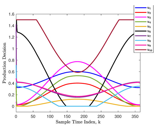
Figure 6.
The optimal decisions at each sample time index.
From the simulation results, Algorithm 1 can be seen to provide the optimal decisions within the constraint at each sample time index to increase the net profit. Therefore, Algorithm 1 achieved the desired practical benefits in solving the production planning problem. Note that the authors employed the alternative solution in Proposition 2 to solve problem (35), providing similar results to those obtained from quadprog.
6. Conclusions and Future Work
This paper focuses on the exact production planning problem with a collaborative mode and unknown information and proposes a machine learning-based MPC algorithm to solve this problem. This problem is defined using a mathematical form using a discrete time system and a net profit cost function. This paper records the historical data under the free decision making condition with a certain degree of decision bias to establish a dataset. A gradient descent machine learning procedure is proposed to estimate the unknown parameter values based on the elements in the dataset, and MPC uses the estimated parameters to make the optimal decisions by solving a quadratic optimization problem at each sample time index. These procedures together yield a comprehensive algorithm for this specific class of production planning problems. The algorithm is validated using a simulation-based case study to check its parameter estimation accuracy and task performance. In addition, a comparison with individual decision making and pure MPC decision making is conducted to show its advantages in terms of increasing profit.
Although the efficiency and effectiveness of the proposed algorithm are shown in this paper, some potential extensions can be made to strengthen the generality and reliability of this method. First of all, a general non-linear system model can be used to broaden the generality to estimate unknown information for other control methods, such as iterative learning control [49,50], and a target task performance other than the net profit is suggested to be considered to achieve alternative benefits. Moreover, a research study on a system with complex dynamic interactions among the participants and associated applications—e.g., a large scale non diagonal Q matrix—are under consideration for future works. Last but not least, other alternative frameworks, such as a real-time optimization framework and Economic MPC, will be further explored to confirm the wide applications of the proposed algorithm in the area of production planning.
Author Contributions
Conceptualization, Y.C.; methodology, Y.C.; software, Y.C.; validation, Y.C.; formal analysis, Y.C.; investigation, Y.Z. (Yueyuan Zhang); resources, Y.C.; writing—original draft preparation, Y.C.; writing—review and editing, Y.C.; visualization, Y.Z. (Yingwei Zhou); supervision, Y.C.; project administration, Y.C.; funding acquisition, Y.C. All authors have read and agreed to the published version of the manuscript.
Funding
This research was funded by the Excellent Young Scholar Program of Soochow University.
Conflicts of Interest
The authors declare no conflict of interest.
References
- Cao, M.; Zhang, Q. Supply chain collaboration: Impact on collaborative advantage and firm performance. J. Oper. Manag. 2011, 29, 163–180. [Google Scholar] [CrossRef]
- Zhang, D.; Shi, P.; Wang, Q.G.; Yu, L. Analysis and synthesis of networked control systems: A survey of recent advances and challenges. ISA Trans. 2017, 66, 376–392. [Google Scholar] [CrossRef]
- Osborne, M.J.; Rubinstein, A. A Course in Game Theory; The MIT Press: Cambridge, MA, USA, 1994. [Google Scholar]
- Park, Y.B. An integrated approach for production and distribution planning in supply chain management. Int. J. Prod. Res. 2005, 43, 1205–1224. [Google Scholar] [CrossRef]
- Huang, S.; Yang, C.; Zhang, X. Pricing and production decisions in dual-channel supply chains with demand disruptions. Comput. Ind. Eng. 2012, 62, 70–83. [Google Scholar] [CrossRef]
- Kopanos, G.M.; Georgiadis, M.C.; Pistikopoulos, E.N. Energy production planning of a network of micro combined heat and power generators. Appl. Energy 2013, 102, 1522–1534. [Google Scholar] [CrossRef]
- Selim, H.; Araz, C.; Ozkarahan, I. Collaborative production-distribution planning in supply chain: A fuzzy goal programming approach. Transp. Res. Part E 2008, 44, 396–419. [Google Scholar] [CrossRef]
- Ma, Y.; Yan, F.; Kang, K.; Wei, X. A novel integrated production-distribution planning model with conflict and coordination in a supply chain network. Knowl.-Based Syst. 2016, 105, 119–133. [Google Scholar] [CrossRef]
- Hu, Z.; Ma, N.; Gao, W.; Lv, C.; Yao, L. Modelling diffusion for multi-generational product planning strategies using bi-level optimization. Knowl.-Based Syst. 2017, 123, 254–266. [Google Scholar] [CrossRef]
- Eduardo, L.; Cardenas-Barron. Economic production quantity with rework process at a single-stage manufacturing system with planned backorders. Comput. Ind. Eng. 2009, 57, 1105–1113. [Google Scholar]
- Zhang, B.; Xu, L. Multi-item production planning with carbon cap and trade mechanism. Int. J. Prod. Econ. 2013, 144, 118–127. [Google Scholar] [CrossRef]
- Gong, X.; Zhou, S.X. Optimal Production Planning with Emissions Trading. Oper. Res. 2013, 61, 908–924. [Google Scholar] [CrossRef]
- Stevenson, M.; Hendry, L.C.; Kingsman, B.G. A review of production planning and control: The applicability of key concepts to the make-to-order industry. Int. J. Prod. Res. 2005, 43, 869–898. [Google Scholar] [CrossRef]
- Wang, L.; Keshavarzmanesh, S.; Feng, H.Y.; Buchal, R.O. Assembly process planning and its future in collaborative manufacturing: A review. Int. J. Adv. Manuf. Technol. 2009, 41, 132–144. [Google Scholar] [CrossRef]
- Maravelias, C.T.; Sung, C. Integration of production planning and scheduling: Overview, challenges and opportunities. Comput. Chem. Eng. 2009, 33, 1919–1930. [Google Scholar] [CrossRef]
- Fahimnia, B.; Farahani, R.Z.; Marian, R.; Luong, L. A review and critique on integrated production-distribution planning models and techniques. J. Manuf. Syst. 2013, 32, 1–19. [Google Scholar] [CrossRef]
- Biel, K.; Glock, C.H. Systematic literature review of decision support models for energy-efficient production planning. Comput. Ind. Eng. 2016, 101, 243–259. [Google Scholar] [CrossRef]
- LeCun, Y.; Bengio, Y.; Hinton, G. Deep learning. Nature 2015, 521, 436–444. [Google Scholar] [CrossRef]
- Hastie, T.; Tibshirani, R.; Friedman, J. The Elements of Statistical Learning; Springer: Berlin, Germany, 2001. [Google Scholar]
- Nasrabadi, N.M. Pattern recognition and machine learning. J. Electron. Imaging 2007, 16, 049901. [Google Scholar]
- Krizhevsky, A.; Sutskever, I.; Hinton, G.E. ImageNet classification with deep convolutional neural networks. In Proceedings of the 2012 International Conference on Neural Information Processing Systems (NIPS), Lake Tahoe, NV, USA, 3–6 December 2012; pp. 1097–1105. [Google Scholar]
- Qi, Z.; Tian, Y.; Shi, Y. Structural twin support vector machine for classification. Knowl.-Based Syst. 2013, 43, 74–81. [Google Scholar] [CrossRef]
- Shao, H.; Jiang, H.; Li, X.; Wu, S. Intelligent fault diagnosis of rolling bearing using deep wavelet auto-encoder with extreme learning machine. Knowl.-Based Syst. 2018, 140, 1–14. [Google Scholar]
- Cai, J.; Luo, J.; Wang, S.; Yang, S. Feature selection in machine learning: A new perspective. Neurocomputing 2018, 300, 70–79. [Google Scholar] [CrossRef]
- Jeon, H.K.; Yang, C.S. Enhancement of Ship Type Classification from a Combination of CNN and KNN. Electronics 2021, 10, 1169. [Google Scholar] [CrossRef]
- Chen, Y.; Zhou, Y. Machine learning based decision making for time varying systems: Parameter estimation and performance optimization. Knowl.-Based Syst. 2020, 190, 105479. [Google Scholar] [CrossRef]
- Mikolov, T.; Sutskever, I.; Chen, K.; Corrado, G.S.; Dean, J. Distributed representations of words and phrases and their compositionality. In Proceedings of the 2013 International Conference on Neural Information Processing Systems (NIPS), Lake Tahoe, NV, USA, 5–10 December 2013; pp. 3111–3119. [Google Scholar]
- Ros, G.; Sellart, L.; Materzynska, J.; Vazquez, D.; Lopez, A.M. The synthia dataset: A large collection of synthetic images for semantic segmentation of urban scenes. In Proceedings of the 2016 IEEE Conference on Computer Vision and Pattern Recognition (CVPR), Las Vegas, NV, USA, 27–30 June 2016; pp. 3234–3243. [Google Scholar]
- Tao, H.; Wang, P.; Chen, Y.; Stojanovic, V.; Yang, H. An unsupervised fault diagnosis method for rolling bearing using STFT and generative neural networks. J. Frankl. Inst. 2020, 357, 7286–7307. [Google Scholar] [CrossRef]
- Samanta, A.; Chowdhuri, S.; Williamson, S.S. Machine Learning-Based Data-Driven Fault Detection/Diagnosis of Lithium-Ion Battery: A Critical Review. Electronics 2021, 10, 1309. [Google Scholar] [CrossRef]
- Garcia, C.E.; Prett, D.M.; Morari, M. Model predictive control: Theory and practice—A survey. Automatica 1989, 25, 335–348. [Google Scholar] [CrossRef]
- Yang, T.; Qiu, W.; Ma, Y.; Chadli, M.; Zhang, L. Fuzzy model-based predictive control of dissolved oxygen in activated sludge processes. Neurocomputing 2014, 136, 88–95. [Google Scholar] [CrossRef]
- Parisio, A.; Rikos, E.; Glielmo, L. A Model Predictive Control Approach to Microgrid Operation Optimization. IEEE Trans. Control Syst. Technol. 2014, 22, 1813–1827. [Google Scholar] [CrossRef]
- Geyer, T.; Quevedo, D.E. Performance of Multistep Finite Control Set Model Predictive Control for Power Electronics. IEEE Trans. Power Electron. 2015, 30, 1633–1644. [Google Scholar] [CrossRef]
- Froisy, J. Model predictive control: Past, present and future. ISA Trans. 1994, 33, 235–243. [Google Scholar] [CrossRef]
- Qin, S.; Badgwell, T.A. A survey of industrial model predictive control technology. Control Eng. Pract. 2003, 11, 733–764. [Google Scholar] [CrossRef]
- Mayne, D.Q. Model predictive control: Recent developments and future promise. Automatica 2014, 50, 2967–2986. [Google Scholar] [CrossRef]
- Mula, J.; Poler, R.; Garcia-Sabater, J.P.; Lario, F.C. Models for production planning under uncertainty: A review. Int. J. Prod. Econ. 2006, 103, 271–285. [Google Scholar] [CrossRef] [Green Version]
- Shi, J.; Zhanga, G.; Sha, J. Optimal production planning for a multi-product closed loop system with uncertain demand and return. Comput. Oper. Res. 2011, 38, 641–650. [Google Scholar] [CrossRef] [Green Version]
- Kenne, J.P.; Dejax, P.; Gharbi, A. Production planning of a hybrid manufacturing-remanufacturing system under uncertainty within a closed-loop supply chain. Int. J. Prod. Econ. 2012, 135, 81–93. [Google Scholar] [CrossRef] [Green Version]
- Wang, Y.; Zhou, D.; Gao, F. Iterative learning model predictive control for multi-phase batch processes. J. Process Control 2008, 18, 543–557. [Google Scholar] [CrossRef]
- Aswani, A.; Master, N.; Taneja, J.; Culler, D.; Tomlin, C. Reducing Transient and Steady State Electricity Consumption in HVAC Using Learning-Based Model-Predictive Control. Proc. IEEE 2012, 100, 240–253. [Google Scholar] [CrossRef]
- Aswani, A.; Sastry, H.G.S.S.; ClaireTomlin. Provably safe and robust learning-based model predictive control. Automatica 2013, 49, 1216–1226. [Google Scholar] [CrossRef] [Green Version]
- Kayacan, E.; Kayacan, E.; Ramon, H.; Saeys, W. Learning in centralized nonlinear model predictive control: Application to an autonomous tractor-trailer system. IEEE Trans. Control Syst. Technol. 2015, 23, 197–205. [Google Scholar] [CrossRef]
- Chen, Y.; Zhou, Y.; Zhang, Y. Collaborative Production Planning with Unknown Parameters using Model Predictive Control and Machine Learning. In Proceedings of the 2020 China Automation Congress (CAC), Shanghai, China, 6–8 November 2020. [Google Scholar]
- James, G.; Witten, D.; Hastie, T.; Tibshirani, R. An Introduction to Statistical Learning; Springer: Berlin, Germany, 2013. [Google Scholar]
- Kohavi, R. A Study of CrossValidation and Bootstrap for Accuracy Estimation and Model Selection. In Proceedings of the 1995 International Joint Conference on Articial Intelligence (IJCAI), Montreal, QC, Canada, 20–25 August 1995; pp. 1137–1145. [Google Scholar]
- Chen, Y.; Chu, B.; Freeman, C.T. Point-to-Point Iterative Learning Control with Optimal Tracking Time Allocation. IEEE Trans. Control Syst. Technol. 2018, 26, 1685–1698. [Google Scholar] [CrossRef] [Green Version]
- Chen, Y.; Chu, B.; Freeman, C.T. Generalized Iterative Learning Control using Successive Projection: Algorithm, Convergence and Experimental Verification. IEEE Trans. Control Syst. Technol. 2020, 28, 2079–2091. [Google Scholar] [CrossRef] [Green Version]
- Chen, Y.; Chu, B.; Freeman, C.T. Iterative Learning Control for Path-Following Tasks With Performance Optimization. IEEE Trans. Control. Syst. Technol. 2021, 1–13. [Google Scholar] [CrossRef]
Publisher’s Note: MDPI stays neutral with regard to jurisdictional claims in published maps and institutional affiliations. |
© 2021 by the authors. Licensee MDPI, Basel, Switzerland. This article is an open access article distributed under the terms and conditions of the Creative Commons Attribution (CC BY) license (https://creativecommons.org/licenses/by/4.0/).