Modeling Radio-Frequency Devices Based on Deep Learning Technique

Abstract

An advanced method of modeling radio-frequency (RF) devices based on a deep learning technique is proposed for accurate prediction of S parameters. The S parameters of RF devices calculated by full-wave electromagnetic solvers along with the metallic geometry of the structure, permittivity and thickness of the dielectric layers of the RF devices are used partly as the training and partly as testing data for the deep learning structure. To implement the training procedure efficiently, a novel selection method of training data considering critical points is introduced. In order to rapidly and accurately map the geometrical parameters of the RF devices to the S parameters, deep neural networks are used to establish the multiple non-linear transforms. The hidden-layers of the neural networks are adaptively chosen based on the frequency response of the RF devices to guarantee the accuracy of generated model. The Adam optimization algorithm is utilized for the acceleration of training. With the established deep learning model of a parameterized device, the S parameters can efficiently be obtained when the device geometrical parameters change. Comparing with the traditional modeling method that uses shallow neural networks, the proposed method can achieve better accuracy, especially when the training data are non-uniform. Three RF devices, including a rectangular inductor, an interdigital capacitor, and two coupled transmission lines, are used for building and verifying the deep neural network. It is shown that the deep neural network has good robustness and excellent generalization ability. Even for very wide frequency band (0–100 GHz), the maximum relative error of the coupled transmission lines using the proposed method is below 3%.

1. Introduction

Electromagnetic (EM) simulation approaches, such as method of moments (MoM), which is a numerical computational method that transforms Maxwell’s equations into integral matrix equations, obtain the EM performance by solving the dense matrix equation. The finite-difference time-domain (FDTD) method solved Maxwell’s equations in an explicit way. Because of its simple, robust nature and ability to incorporate a broad range of non-linear materials and devices, FDTD is often used to study a wide range of applications, including antenna design, microwave circuits, bio/EM effects, and photonics. The finite element method (FEM) transforms Maxwell’s equations into differential equations. The FEM solver can handle arbitrary shaped structures, like bond wires, conical shape vias, and solder bumps, and dielectric bricks or finite-size substrates. Although these EM simulation methods are powerful for RF device analyses these approaches suffer from a severe problem, i.e., they are very time consuming. Some studies have used artificial neural network (ANN) for assessment of electromagnetic field radiating by electrostatic discharges [1] or design of microwave circuits [2]. In these studies, shallow neural networks (with only one hidden layer in neural network) have been used. Some recent studies [3,4] revealed that the capability of shallow neural networks is very limited by comparison with deep neural networks (DNNs). Neural networks that contain only one or two hidden layers cannot fit complex training data well, especially when the dataset is non-uniform or contains missing values. On the other hand, optimization algorithms, such as stochastic gradient descent (SGD), Newton’s method, or Levenberg–Marquardt (LM) algorithm, have been used for the training process. However, these optimization methods are still unsuitable for deep learning training, in which there are a large amount of training data and complex neural network structures. The datasets used by these previous studies have been collected by uniform sampling or dense sampling. Whether the neural networks have enough generalization ability for non-uniform sampling training data has not been discussed.

With the continuous upgrading of the equipment needed to train neural networks and the advent of the big data era, traditional shallow ANN has been gradually transforming into DNN, such as basely fully connected network, convolutional neural network (CNN), and recurrent neural network (RNN). DNN is able to model RF devices with the data collected from accurate EM simulations by mapping the geometry information and frequency of the RF devices to the scattering parameters (or S-parameters, they describe the electrical behavior of linear electrical networks when undergoing various steady state stimuli by electrical signals [5]). DNN can extract more features in each layer from the training data by comparison with shallow ANN. The model generated from DNN can be used for rapidly generating the S parameters of the parameterized RF device, which can avoid the long CPU time of performing the rigorous EM simulation.

On the other hand, there are many classic optimization algorithms to training the neural network, such as stochastic gradient descent (SGD) [6], Newton’s method [7] or Levenberg–Marquardt (LM) algorithm [8]. However, they all have some drawbacks, which cause them not suitable for training DNN in various ways.

The SGD algorithm can guarantee the global optimal solution only when the loss function is a convex function [9]. However, the ideal convex function is almost impossible in realistic. Moreover, the SGD also cannot adjust the learning rate automatically. As a consequence, the SGD has poor training speed if the learning rate is set too small. On the other hand, if the learning rate has been set too large, the training process may never reach to the minimum. In addition, the SGD is also prone to be trapped in a saddle point and local minima. Newton’s method needs to calculate Hessian matrix and inverse matrix, implying that it needs more computational resources. If the number of the training data and the size of the neural network are very large, the Jacobian matrix can become huge [10]. Therefore, the Levenberg–Marquardt algorithm is not suitable for big data models.

As a recently proposed optimization algorithm, advanced optimization algorithm (Adam) [11] has advantages in memory requirements, adaptive learning rates for different parameters, and non-convex optimizations for large datasets and high dimensional spaces.

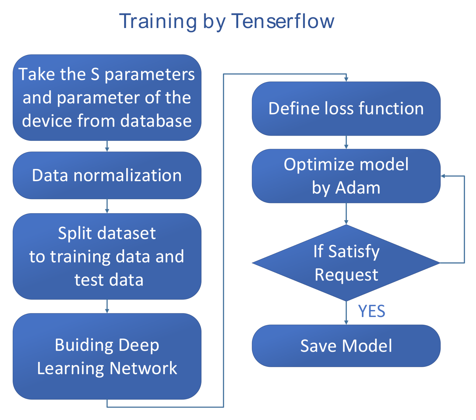
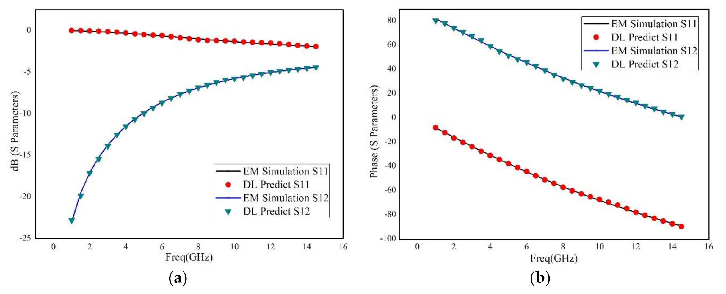
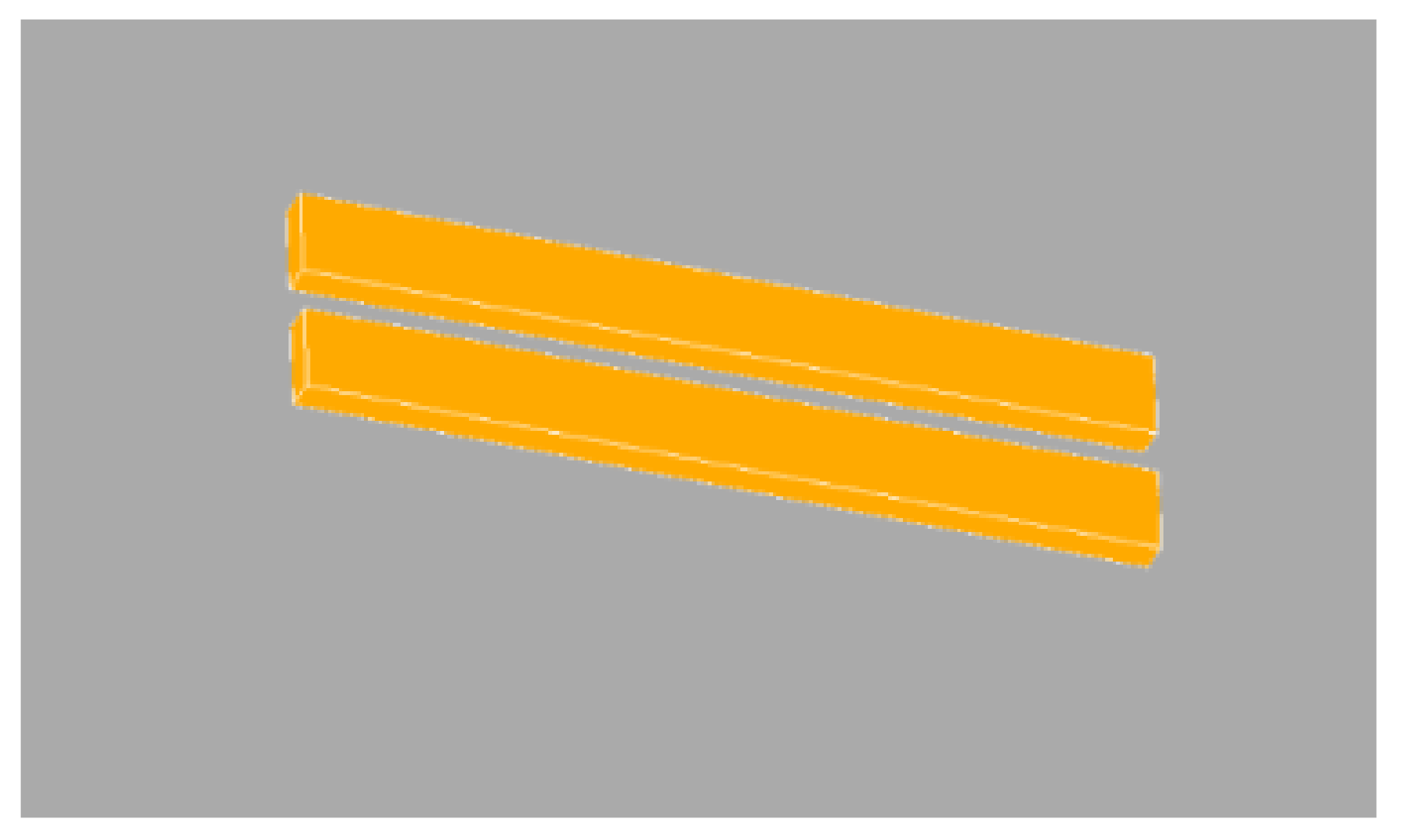
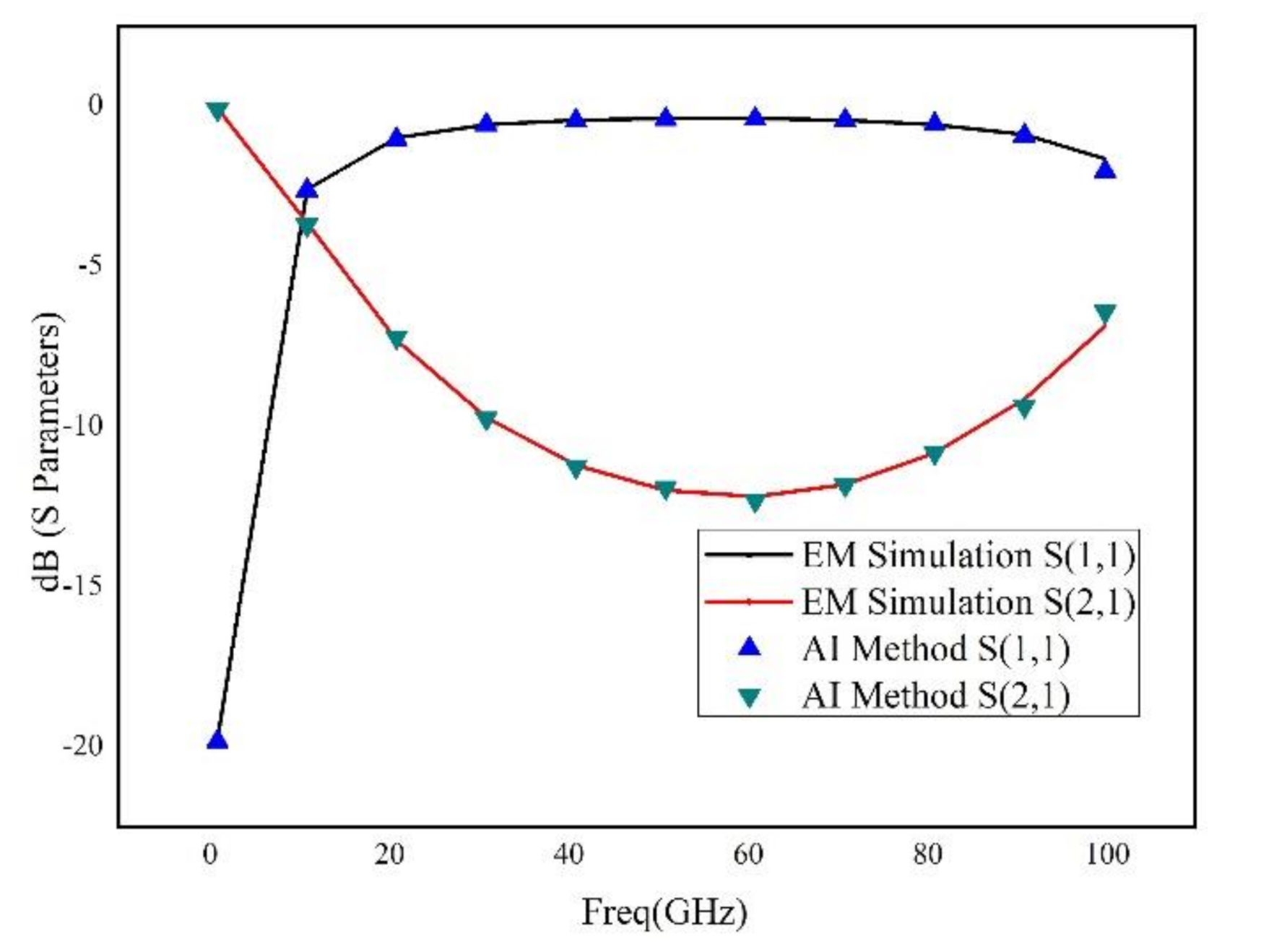
In this work, the DNN modeling approach, which combines Tensorflow deep learning structure and the training by Adam, is proposed. Not only the metallic geometry of the structure, but also the permittivity and thickness of the dielectric layers are revised during the sweeping process. Accurate prediction of the frequency response can be obtained by this proposed method. During the training procedure, a novel selection method of training data considering critical points is introduced, especially when the training dataset is too large, to enhance the training efficiency. In addition, the layers of the neural networks are adaptively chosen based on the frequency response of the RF devices to generate an optimal model for the RF devices. Three RF devices are used as examples to illustrate this modeling approach. A rectangular inductor is used to build and train the DNN, while an interdigital capacitor is used for validating the generalization ability of the DNN. Finally, an example of two coupled transmission lines is used to validate the accuracy of this method in a very wide frequency band range.

2. Build Neural Network and Define Loss Function

The outline of this work is shown in Figure 1. The feedforward process of deep neural network is shown in Figure 2. In Figure 2, the layer type used herein is the type of fully-connected layer in which the neurons between two adjacent layers are fully pairwise connected, but the neurons within a single layer do not share any connections.

Figure 1. Outline flowchart of this work.

Figure 2. Feedforward process of deep neural network adopts multi-layer fully connected structure. The input data X of the neural network is the geometric parameters and the operating frequency of RF devices, whereas the output data Y are the real part and the imaginary part of the S parameter.

The neural network consists of one input layer, multiple hidden layers that contain certain numbers of units, and one output layers. The function of this neural network is given as:

$$y=\phi \left(W^{n+1}\dots \phi \left(W^2\phi \left(W^{1}x+b^1\right)+b^2\right)\dots +b^{n+1}\right)$$

(1)

denotes the bias vector of the i-th layer. The number of input nodes is equal to the number of geometrical parameter and layer data of layout of RF devices. The number of output nodes is equal to the number of real part and image part of S-parameter. The number of neurons in each layer could be adjusted from 20 to 100; The number of layers could be adjusted from 2 to 7(for the discuss the different of performance influenced by hidden layer. Each layer use dropout method (20% dropout) to avoid overfitting.

Define Loss Fuction

The minimization of loss function defines the goal of the optimization and, thus, has strong impact on the neural network to be built. As the estimation of the S parameters is a regression problem, the loss function can be defined in terms of mean squared error (MSE) as follows:

$$MS{E}_{\left(y, y^{’}\right)}=\frac{{{\displaystyle \sum }}_{i=1}^n{\left(y_i-y_i^{’}\right)}^2}{n}$$

(2)

where $y_i$ is the expected value, and $y_i^{’}$ is the estimation given by the neural network.

3. Modeling of RF Devices

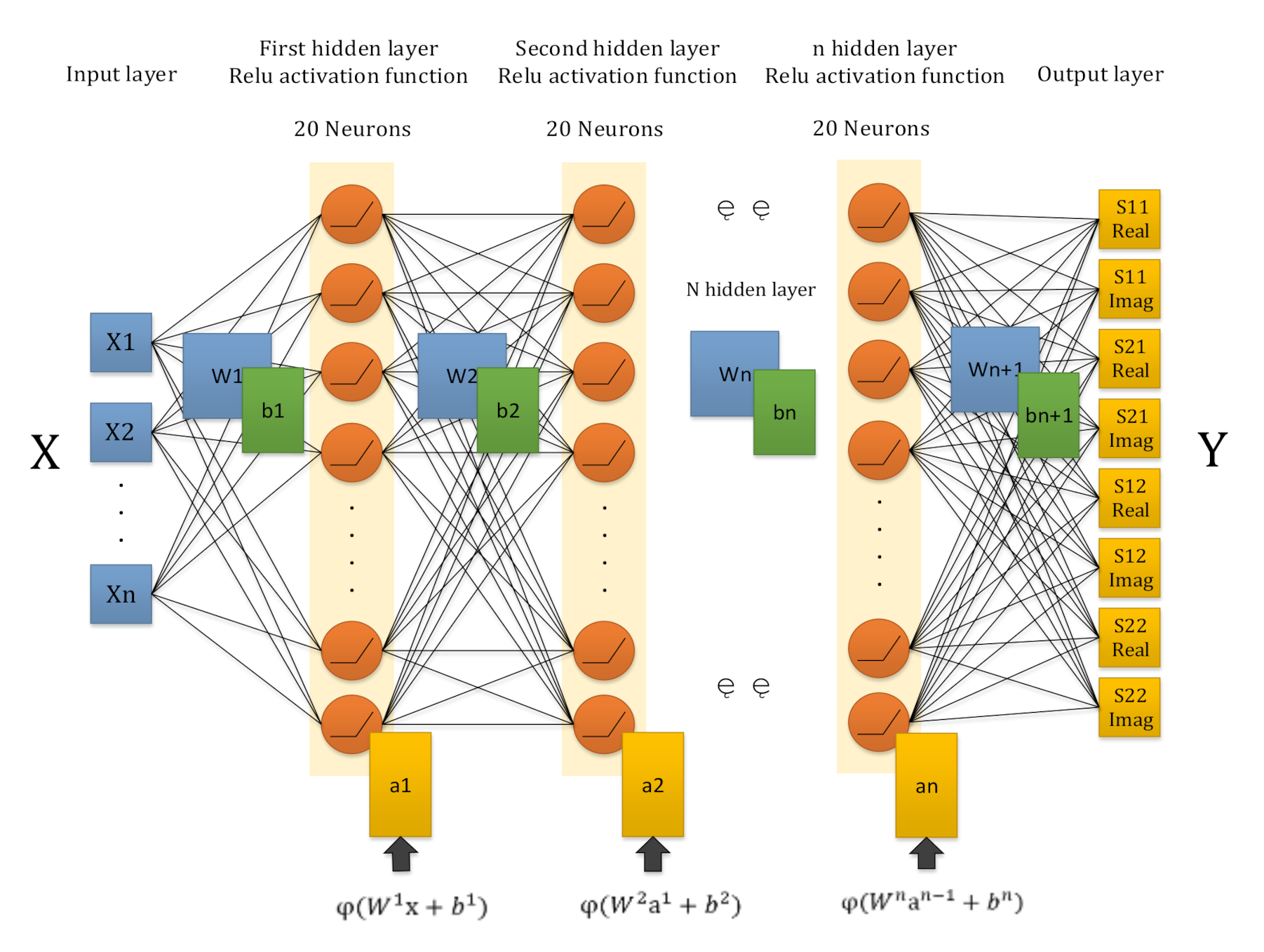
In order to illustrate the DNN-based modeling procedure, two classic RF devices are used: rectangular inductor and interdigital capacitor. The geometrical parameters of the RF device are used as the input data of the neural network, while the S parameters of the RF device is the output of the neural network.

3.1. RF Devices

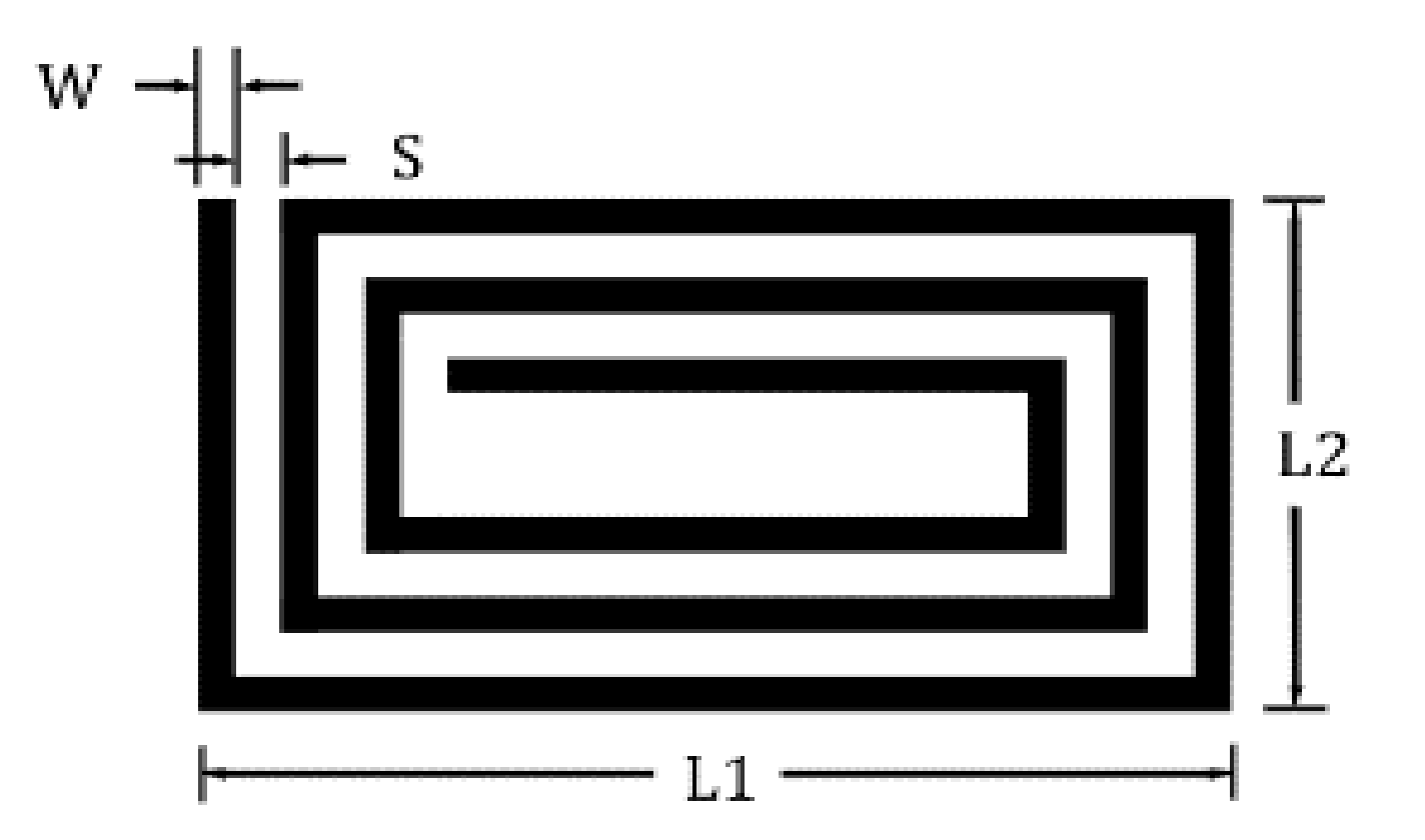
A rectangular inductor, shown in Figure 3, is firstly used to establish the neural network. Its geometrical parameters are listed in Table 1.

Figure 3. Geometrical layout of the planar spiral inductor.

Table 1. Parameter of microstrip rectangular inductor.

Name	Definition	Units
W	Conductor width	mil
S	Conductor spacing	mil
N	Number of turns	None
L1	Length of second outermost segment	mil
L2	Length of outermost segment	mil

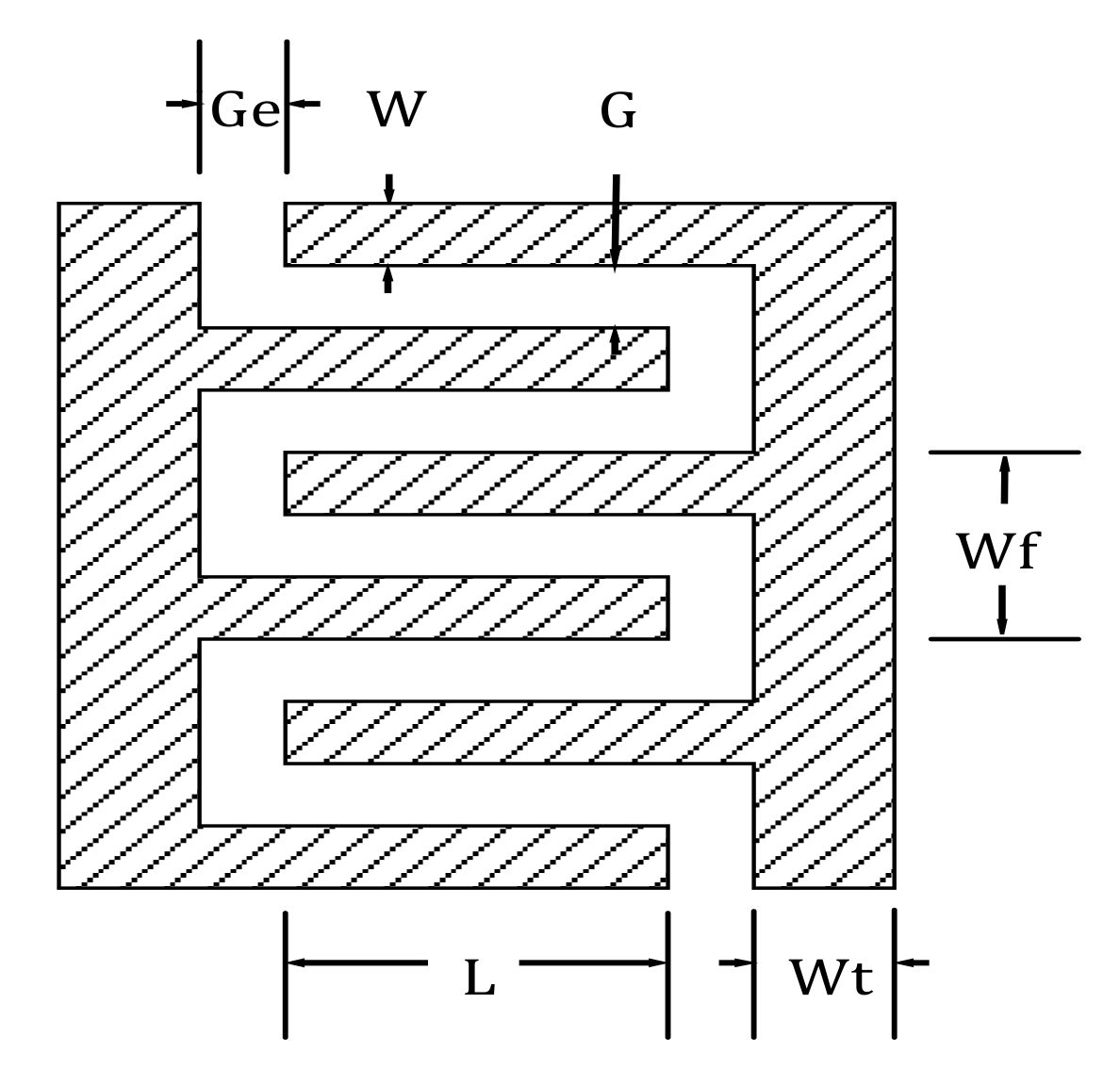
Interdigital capacitor, as shown in Figure 4, is used to test and verify the accuracy and generalization of the neural network. Its geometrical parameters are listed in Table 2.

Figure 4. Geometry layout of the microstrip interdigital capacitor.

Table 2. Parameter of microstrip interdigital capacitor.

Name	Definition	Units
W	Finger width	mil
G	Gap between fingers	mil
Ge	Gap at end of fingers	None
L	Length of overlapped region	mil
Np	Number of finger pairs	Integer

The input and output parameters of the deep neural network with these two RF devices is shown in the Table 3.

Table 3. Input and output of deep neural network.

Device Name	Input Parameters	Output Parameters
rectangular inductor	L1	S11(real and imaginary part)
	L2	S12(real and imaginary part)
	Frequency	S21(real and imaginary part)
		S22(real and imaginary part)
Interdigital	G	S11(real and imaginary part)
	Ge	S12(real and imaginary part)
	L	S21(real and imaginary part)
	Np	S22(real and imaginary part)
	Frequency

3.2. Dataset and Feature Scaling

In order to verify the accuracy and generalization ability of the trained model, two training datasets are taken from the EM simulation. The first dataset uses uniform sampling data (see Table 4) the total number of instances is 2421, whereas the second dataset uses non-uniform sampling data (see Table 5) the total number of instances is 1156.

Table 4. Uniform sampling of rectangular inductor.

L1 (Mil)	L2 (Mil)	Frequency (GHz)
30–40 (step = 1)	15–25 (step = 1)	1–20 (step = 1)

Table 5. Non-uniform sampling of rectangular inductor.

L1 (Mil)	L2 (Mil)	Frequency (GHz)
30–33 (step = 1.5)	15–17.5 (step = 0.5)	1–5 (step = 0.5)
36–37 (step = 0.5)	20–22 (step = 0.2)	7–13 (step = 3)
38–40 (step = 2)	23–25 (step = 2)	14–15 (step = 0.2)
		16–20 (step = 2)

In order to prove deep learning has the capability to handle complex dataset and make accurate prediction, the step and gap in the second dataset are chosen randomly. Before applying the training data to the neural network, the original dataset needs to be preprocessed. In Table 4 and Table 5, the range of the input parameters are different from one another. Thus, normalization is highly necessary for the training data. If no normalization is performed, some parameters vary greatly while other parameters have very small ranges of variations. As a consequence, the parameters have different effects on the weighting term and the bias term, thereby leading to continuous adjustment of the learning rate during optimization and causing the training gradient to fall in a “zigzag” manner, which results in very low training efficiency and even makes the training difficult to perform.

Pretreated by the normalization, the speed of the optimization algorithm for training the deep neural network can be effectively accelerated, and the accuracy can be also highly improved. The min–max normalization, which is often known as the feature scaling, is used herein, in which the values of a numeric range of a feature of data, i.e., a property, are compressed to a scale between −1 and 1.

Moreover, the original dataset needs to be divided into a training data and a testing data. The raw dataset is randomly shuffled and then 80% of it is assigned as a training data while 20% as a testing data [12]. Table 6 lists a randomly chosen test data for the rectangular inductor.

Table 6. Test data of rectangular inductor.

L1 (Mil)	L2 (Mil)	Frequency (GHz)
34.56	22.375	1–20 (step = 0.5)

3.3. Training Process

The backpropagation is the core method to training the neural network. It can optimize the weights and biases in the neural network according to the defined loss function in each epoch, so that the resulted loss function can reach a small value.

As mentioned before, many advanced optimization algorithms have been proposed. Herein, the Adam algorithm is used for optimization, which is formulated as follows:

$$m_t={\beta }_1{m}_{t-1}+\left(1-{\beta }_1\right)g_t$$

(3)

$$v_t={\beta }_2{v}_{t-1}=\left(1-{\beta }_2\right)g_t^2$$

(4)

$${\widehat{m}}_t=\frac{m_t}{1-{\beta }_1^t}$$

(5)

$${\widehat{v}}_t=\frac{v_t}{1-{\beta }_2^t}$$

(6)

$${\theta }_{t+1}={\theta }_t-\frac{\eta }{\sqrt{{\widehat{v}}_t+\epsilon }}{\widehat{m}}_t$$

(7)

where $g_t$ is the gradient of the loss function at the t-th iteration, ${\beta }_1$ and ${\beta }_2$ are the delay factors,$m_t$ and $v_t$ are the biased first moment estimate and the biased second raw moment estimate of the gradient, respectively, ${\widehat{m}}_t$ and ${\widehat{v}}_t$ are the bias-corrected first moment estimate and the bias-corrected second raw moment estimate, respectively, ${\theta }_{t+1}$ is the updated parameter of ${\theta }_t$, and $\eta$ and $\epsilon$ are two constants.

In the optimization of the loss function, the Adam optimization algorithm uses the iteration number and the delay factor to correct the gradient mean and the gradient square mean, accelerate the learning speed and efficiency, and adjust the learning rate automatically. Good default settings for the tested machine learning problems are $\eta$ = 0.001,${\beta }_1$ = 0.9, ${\beta }_2$ = 0.999 and $\epsilon$ = ${10}^{-8}$.

The Adam optimization algorithm combines Adagrad’s [13] advantage in dealing with sparse gradients and RMSprop’s ability to handle non-stationary targets. With less memory requirements, it calculates different adaptive learning rates for different parameters, and is also suitable for most non-convex optimizations for large datasets and high dimensional spaces.

4. Result and Discussion

The modeling procedure is as follows: (1) Feed the training data into the neural network to start the training; (2) Utilize the optimization algorithm to update the weights and the biases until the training loss drops below 1%; (3) Feed the testing data into the neural networks and calculate the test loss. These processes will keep repeating until the test loss drops to the goal 0.1%, or the epochs reach to the maximum number 100,000.

4.1. Uniform Sampling

For the uniform sampling case, as shown in Table 7, the resulted neural network contains 2 hidden layers and 20 neurons in each layer, and the test loss reach to goal. Figure 5 compares the results of the deep learning with those from the EM simulation. Not surprisingly, the results predicted by the deep learning agree very well with those from the EM simulation.

Table 7. Train and test loss of neural network.

Hidden Layer Number	Neuron Number in Each Layer	Train Loss	Test Loss
2	20	$7.058\times {10}^{-5}$	$9.989\times {10}^{-5}$

Figure 5. Results of the deep learning versus those from the EM simulation for uniformly sampling. The results of the deep learning are denoted by dots, while the results from the EM simulation are shown by solid lines (a) dB of S Parameters. (b) Phase of S Parameters.

4.2. Non-Uniform Sampling

For the non-uniform sampling case, three neural networks and their corresponding train and test losses are shown in Table 8. For the neural network with 2 hidden layers and 20 neurons on each layer, the test loss does not reach to the goal after 100,000 epochs. As shown in Figure 6 the model trained by this neural network does not perform well in comparison with the EM simulation. Therefore, the complexity of the neural network needs to increase.

Table 8. Train and test loss of neural network.

Hidden Layer Number	Neuron Number in Each Layer	Train Loss	Test Loss
2	20	$3.089\times {10}^{-4}$	$3.498\times {10}^{-4}$
2	100	$2.317\times {10}^{-5}$	$9.993\times {10}^{-5}$
5	20	$1.318\times {10}^{-5}$	$8.799\times {10}^{-5}$

Figure 6. Results of the deep learning versus the EM simulation for non-uniformly sampling when a 2-hidden-layer neural network with 20 neurons on each layer is used. (a) dB of S Parameters. (b) Phase of S Parameters.

There two common ways to increase the complexity of neural network: (i) increase the number of neurons on each layer or (ii) add more layers. Firstly, the number of neurons on each layer increases to 100, as shown in the second row of Table 8. By so doing, the train and test losses are significantly reduced (e.g., both drop below 0.1%). However, the actual model results, which are shown in Figure 7, do not exhibit satisfactory performance. The results by the deep learning model do not agree well with those from the EM simulation, particularly in the frequency band where the samples used for training are sparse.

Figure 7. Results of the deep learning versus the EM simulation for non-uniformly sampling when a 2-hidden-layer neural network with 100 neurons on each layer is used. (a) dB of S Parameters. (b) Phase of S Parameters.

It is now well known that shallow neural network may not be able to extract as many features as deep neural network does [3]. Hence, the number of hidden layers is then added to 5 while the number of neurons on each layer is still kept as 20, as shown in the third row of Table 8. The train and test losses are shown in Table 8, and the results of the DNN with 5 hidden layers and 20 neurons on each layer are compared with those from the EM simulation in Figure 8. From Figure 8, one can observe that the DNN with 5 hidden layers has excellent performance in the entire frequency band.

Figure 8. Results of the deep learning versus the EM simulation for non-uniformly sampling when a 5-hidden-layer neural network with 20 neurons on each layer is used. (a) dB of S Parameters. (b) Phase of S Parameters.

The results illustrate that deeper neural network is more effective in RF device modeling. Many previous works have also shown that deep neural network can perform better than the shallow one [14,15]. One of the reasons why deep network is better than shallow network can be explained by “modularization” [16]. Just like computer programing, no programmer would put all of the codes in the main function. Instead, the programmer would separate the program into many sub-functions that content different features of the program. Deep neural network somehow does the same thing. Each layer extracts different feature from the previous layer, and multiple layers correspond to multiple levels of features. The level of abstraction increases with each level and deeper neural network enables discovering and representing higher-level abstractions. This attribution of deep neural network is very important for training the complex input data that are non-uniform, sparse, or even contain missing values. Because the number of samples in this kind of data is very small, acquiring sufficiently detailed features from small number of data is very hard for only one or two layers. This is the reason why the 2-hidden-layer neural network cannot perform well in the high frequency band even if the number of neurons on each layer has been greatly increased.

Another reason to use deep neural network rather than shallow neural network is as follows. Although the deep neural network is large in size and, thus, has more local minimums, they are high-quality low-index critical points that lie close to the global minimum [17,18]. On the other hand, although shallow neural network is small in size, and may have small number of local minimums, its optimization can easily stick in poor local minimum.

4.3. Test and Verification

The interdigital capacitor is used as an example to verify the generalization ability of DNN in the RF device modeling. The DNN, which consists of 5 hidden layers and 20 neurons on each layer and is the best performer as illustrated in preceding subsection for the case of rectangular inductor, is used for the test and verification. Similar to the case of rectangular inductor, the step and gap of the dataset are randomly selected. The sampling of training data is non-uniform and listed in Table 9. The test data are shown in Table 10.

Table 9. Non-uniform sampling of interdigital capacitor.

G (Mil)	Ge (Mil)	L (Mil)	Np	Frequency (Mil)
1–2	1–3	40–42	5–10	1–5
(step = 0.5)	(step = 2)	(step = 0.2)	(step = 1)	(step = 2)
3–4	3.5–4.5	43–45		6–9
(step = 1)	(step = 0.1)	(step = 2)		(step = 0.5)
4.3–5	4.6–5	47–50		11–15
(step = 0.1)	(step = 0.2)	(step = 1.5)		(step = 1)

Table 10. Test data of interdigital capacitor.

G (Mil)	Ge (Mil)	L (Mil)	Np
2.23	3.25	43.24	7

The train and test losses are shown in Table 11. Figure 9 compares the results of the DNN with 5 hidden layers and 20 neurons on each layer and those from the EM simulation. From Figure 9, one can observe that the DNN with 5 hidden layers has excellent performance for the case of interdigital capacitor, implying that the proposed DNN can be used to model other RF devices.

Table 11. Train and test loss of neural network.

Hidden Layer Number	Neuron Number in Each Layer	Train Loss	Test Loss
5	20	$2.970\times {10}^{-5}$	$3.458\times {10}^{-5}$

Figure 9. For interdigital capacitor modeling, results of the deep learning versus the EM simulation for non-uniformly sampling when a 5-hidden-layer neural network with 20 neurons on each layer is used. (a) dB of S Parameters. (b) Phase of S Parameters.

4.4. Adaptive Sampling and Layer Selection

In order to further show the advantage of this work, coupled transmission lines has been tested. The layout of the coupled transmission lines is shown in Figure 10. The parameters used for training are shown in Table 12, which is more complicated than that in Reference [19]. Dissimilarly, only the metallic geometry is used in Reference [19], the dielectric layer information (including the dielectric constant (${\epsilon }_r$) and thickness of dielectric layer) is also set as training parameters herein. The simulation frequency range is set from 1 GHz to 100 GHz.

Figure 10. The layout of coupled transmission lines.

Table 12. Parameter of coupled transmission line.

Name	Definition	Units
W1	Width of line one	µm
W2	Width of line two	µm
Ge	Gap between two lines	µm
L	Length of two lines	µm
Thickness_c	Thickness of conductor layer	µm
Thickness_d	Thickness of dielectric layer	µm
${\epsilon }_r$	Dielectric constant	None

The sweep setting of coupled transmission lines is shown in Table 13. In this example, the number of instances of the fully sweeping dataset is 1,500,000, which is a very large number. In total, 40,000 samples (40,000 is a number chosen from experiment, which can maintain the accuracy of model and reduce the simulation time at the same time) are randomly chosen from the fully sweeping set, and 2000 corner points are additionally chosen to guarantee the accuracy of the model. In the training process, the number of hidden layers is adaptively chosen. In this example, the number of hidden layers is adjusted from 2 to 7 and neurons of each layer are adjusted from 50 to 100. Setting the starting neural network as 2 layers with 50 neurons on each layer. If the mean square error at the end of each round of training does not reach the target loss, one more layer is then automatically added and the new neural network is retrained. If the number of layers added reaches 7 and the target loss is still not reached, the number of neurons of each layer is automatically increased from 50 to 100 and the neural network restarts from 2 layers. In this case, it uses 5 layers with 100 neurons of each layer in the training process to produce an optimal model. The test loss (mean square error) at the end of training is only 8.97 × 10⁻⁵. The randomly chosen testing data and relative error are shown in Table 14. The comparison of S-parameter(dB) between AI method and EM simulation is shown in Figure 11.

Table 13. Sweep setting of coupled transmission lines.

Name	Sweep Setting
W1	10–100 um (step = 10 µm)
W2	10–100 um (step = 10 µm)
Ge	10–100 um (step = 10 µm)
L	100–1 mm (step = 100 µm)
Thickness_c	1–5 um (step = 1 um)
Thickness_d	5–10 um (step = 1 um)
${\epsilon }_r$	5–10 (step = 1)

Table 14. Testing data of coupled transmission lines.

W1	W2	Ge	L	Thickness_c	Thickness_d	${\mathit{\epsilon }}_{\mathit{r}}$	Relative Error	Freq with Max Error
56	56	58	580	3	7.5	3	1.25%	61 GHz
60	60	58	580	3	7.5	3	1.07%	61 GHz
80	50	50	550	3	7	3	1.13%	61 GHz
55	55	55	101	3	7.5	3	1.16%	51 GHz
57	57	57	570	3	7.6	1.1	2.93%	100 GHz

Figure 11. The comparison of dB (S Parameters) between AI method and EM simulation.

4.5. Limitations and Future Work

The mean limitation of this work is the generation of the dataset. The parameters sweeping process of EM simulation can be very time consuming if the number of input parameters is large. For example, if there are 9 input parameters, each parameter has 10 samples to be swept. The total number of EM simulation would be 10⁹. It is a very large number which will cost a lot of time to finish the simulation process. In future work a more affective sample method needed to be propose to reduce the number of sampling and maintaining the accuracy at the same time.

5. Conclusions

An advanced method of modeling RF devices based on deep learning has been proposed. Using Tensorflow deep learning structure, the deep neural network has been constructed, which has significant advantage over the shallow neural network. The Adam optimization algorithm has been adopted, which makes the training more effectively and accurately. In addition, not only the metallic geometry of the structure, but also the permittivity and thickness of the dielectric layers are revised during the sweeping process. Moreover, a novel selection method of training data considering critical points was introduced, and an adaptive method for adjusting the number of hidden-layer of the neural networks based on the frequency response was proposed, which can significantly reduce the time of training procedure and guarantee the accuracy of generated model. Three RF devices, including a rectangular inductor, an interdigital capacitor and two coupled transmission lines, are used for building and verifying the deep neural network. The results illustrated that the deep neural network has good robustness and excellent generalization ability. Even for very wide frequency band prediction, the proposed method has very small relative error by comparison to the brute-force full-wave results.

References

- Fotis, G.P.; Ekonomo, L.; Maris, T.I.; Liatsis, P. Development of an artificial neural network software tool for the assessment of the electromagnetic field radiating by electrostatic discharges. IET Sci. Meas. Technol. 2007, 1, 261–269. [Google Scholar] [CrossRef]
- Goasguen, S.; El-Ghazaly, S.M. A Coupled FDTD-Artificial Neural Network Technique for Large-Signal Analysis of Microwave Circuits. Int. J. RF Microw. Comput. Aided Eng. 2002, 12, 25–36. [Google Scholar] [CrossRef]
- Mhaskar, H.N.; Poggio, T. Deep vs. shallow networks: An approximation theory perspective. CBMM Memo 2016, 829–848. [Google Scholar] [CrossRef]
- Bengio, Y. Learning Deep Architectures for AI. Found. Trends Mach. Learn. 2009, 2, 1–55. [Google Scholar] [CrossRef]
- Wang, G.; Zhao, P.; Zhang, Z.; Shi, H. An artificial intelligence based electromagnetic simulation method and electromagnetic brain. Chinese Patent Application 201,711,439,836.1, 19 June 2018. [Google Scholar]
- Ruder, S. An overview of gradient descent optimization algorithms. arXiv 2017, arXiv:1609.04747v2. [Google Scholar]
- Polyak, B.T. Newton’s method and its use in optimization. Eur. J. Oper. Res. 2007, 181, 1086–1096. [Google Scholar] [CrossRef]
- Lourakis, M.I.A. A Brief Description of the Levenberg-Marquardt Algorithm Implemented by Levmar; Technical Report; Institute of Computer Science, Foundation for Research and Technology-Hellas: Heraklion, Greece, 2005. [Google Scholar]
- Dauphin, Y.N.; Pascanul, R.; Gulcehre, C.; Cho, K.; Ganguli, S.; Bengio, Y. Identifying and attacking the saddle point problem in high-dimensional non-convex optimization. arXiv 2014, arXiv:1406.2572v1. [Google Scholar]
- Martin, T.; Mohammad, H.; Menhaj, B. Training Feedforward Networks with the Marquardt Algorithm. IEEE Trans. Neural Netw. 1994, 5, 989–993. [Google Scholar]
- Kingma, D.P.; Ba, J.L. Adam: A method for stochastic optimization. arXiv 2017, arXiv:1412.6980v9. [Google Scholar]
- Géron, A. Create a Test Set. In Hands-On Machine Learning with Scikit-Learn and TensorFlow, 1st ed.; O’Reilly Media: Oxford MA, USA, 2017; pp. 75–78. [Google Scholar]
- Duchi, J.; Hazan, E.; Singer, Y. Adaptive subgradient methods for online learning and stochastic optimization. J. Mach. Learn. Res. 2011, 12, 2121–2159. [Google Scholar]
- Seide, F.; Li, G.; Yu, D. Conversation speech transcription using context-deep neural networks. In Proceedings of the 29th International Conference on International Conference on Machine Learning, Edinburgh, Scotland, 26 June–21 July 2012; pp. 1–2. [Google Scholar]
- Mhaskar, H.; Liao, Q.; Poggio, T. When and why are deep networks better than shallow ones? In Proceedings of the AAAI-17: Thirty-First AAAI Conference on Artificial Intelligence, San Francisco, CA, USA, 4–9 February 20107; pp. 2343–2349. [Google Scholar]
- Zeiler, M.D.; Fergus, R. Visualizing and understanding convolutional networks. In Computer Vision–ECCV; Springer: Cham, Switzerland, 2014; pp. 818–838. [Google Scholar]
- Choromanska, A.; Henaff, M.; Mathieu, M.; Arous, G.B.; LeCun, Y. The loss surfaces of multilayer networks. J. Mach. Learn. Res. 2015, 38, 192–204. [Google Scholar]
- Pennington, J.; Bahri, Y. Geometry of neural network loss surfaces via random matrix theory. In Proceedings of the 34th International Conference on Machine Learning, Sydney, Australia, 6–11 August 2017; Volume 70, pp. 2798–2806. [Google Scholar]
- Plonis, D.; Katkevičius, A.; Gurskas, A. Predicting the Frequency Characteristics of Hybrid Meander Systems Using a Feed-Forward Backpropagation Network. Electronics 2019, 8, 85. [Google Scholar] [CrossRef] [Green Version]
Publisher’s Note: MDPI stays neutral with regard to jurisdictional claims in published maps and institutional affiliations. |
© 2021 by the authors. Licensee MDPI, Basel, Switzerland. This article is an open access article distributed under the terms and conditions of the Creative Commons Attribution (CC BY) license (https://creativecommons.org/licenses/by/4.0/).