Evaluation of Transmission Properties of Networks Described with Reference Graphs Using Unevenness Coefficients ^†

Abstract

This paper discusses an evaluation method of transmission properties of networks described with regular graphs (Reference Graphs) using unevenness coefficients. The first part of the paper offers generic information about describing network topology via graphs. The terms ‘chord graph’ and ‘Reference Graph’, which is a special form of a regular graph, are defined. The operating principle of a basic tool used for testing the network’s transmission properties is discussed. The next part consists of a description of the searching procedure of the shortest paths connecting any two nodes of a graph and the method determining the number of uses of individual graph edges. The analysis shows that using particular edges of a graph depends on two factors: their total number in minimum length paths and their total number in parallel paths connecting the graph nodes. The latter makes it possible to define an unevenness coefficient. The calculated values of the unevenness coefficients can be used to evaluate the transmission properties of networks and to control the distribution of transmission resources.

1. Introduction

A basic problem faced by designers of ICT networks is the selection of a topology of internodal connections that will guarantee the best efficiency and reliability of information transfer, that is, a topology in which both the diameter and the average length of the paths of the graph describing the lattice reach their minimum values. The aim of this study is to analyze the transmission properties of ICT networks described with graphs whose nodes are modules acting as commutators and whose edges are transmission channels connecting the nodes. This paper includes the analysis and results of the possibility of utilizing the unevenness coefficients of the use of individual graph edges for the assessment of the transmission properties of networks described with these graphs. ICT networks must fulfil the requirements of adequate quality, rate, and reliability of information transmission. Therefore, apart from the selection of proper hardware to be installed in their nodes, the correct setup of connections between the parts of the network [1,2,3,4,5,6,7,8] is taken into consideration. The main purpose of ICT systems design is to reach the following:

• The minimum network connection cost presented as the total number of links;
• The minimum communication delay—the representation of this parameter is the size of the diameter and the average path length;
• A substantial fault tolerance characterized by the number of independent paths between two nodes (connectivity) or the minimum number of nodes or edges after the removal of which the networks is no longer consistent (node and edge connectivity);
• Regularity and symmetry;
• Ease of routing;
• Extensibility.

Network topologies can be described using graphs [1,9,10]. Their vertices (nodes) can be commutation modules or specialized computers. The edges are usually two-way, independent transmission channels linking these vertices. Fiber-optic cables are most commonly used to transmit information in extended ICT networks, and these networks generally have a ring structure [11,12]. The transmission characteristics of a standard ring structure are not satisfactory; therefore, to improve it, it is modified by the introduction of additional internodal connections called chords. The structures obtained in such a way are called chordal rings [13].

Definition 1.

The chordal ring is a special case of a circulant graph defined by the pair $(p,Q)$, where p denotes the number of nodes and Q the set of chords, $Q\subseteq \{1,2,\dots ,\lfloor p/2\rfloor \}$. Each of the chords $q_i\in Q$ connects a pair of nodes included in the ring, where $q_i$ denotes the length of the chord equal to the number of the ring edges between the nodes. The chord ring is described by the notation $G(p;q_1,\dots ,q_i)$, where $q_1=1<q_2<\cdots <q_i$. The degree of nodes is generally equal to d(V) = 2i, except when the chord length is $p/2$; in this case, p and the node degree is 2i-1 [14].

Many publications [14,15,16,17,18,19] show that the diameter and average path length have a significant influence on the transmission properties of the network modelled by graphs. To objectively evaluate the minimal values above the given basic parameters of the analyzed connection typologies, the Reference Graphs were established [20,21,22].

Definition 2.

Reference Graphs are the regular structures with a predetermined number of nodes in which the diameter values and the average path lengths from any source node reach the same, theoretically calculated lower size limits.

Amongst Reference Graphs (RG) are ideal and optimal graphs that depend on the number of nodes forming these graphs. An optimal graph is a structure in which all sets of nodes equally distant from the source node (called ‘layers’) reach the maximum count, while in an ideal graph, the set of nodes furthest from the node (the last layer) does not fulfil this condition. The authors in [23] describe an algorithm that made it possible to develop software for research aiming at the verification of whether structures of this kind truly exist. The above-mentioned software was modified, which helped to achieve sets of Reference Graphs with various configurations and with the predetermined number and degree of nodes.

2. The Adopted Method of Analyzing the Topic

In the above-mentioned publications, the method of searching such structures was described. Preliminary simulation studies of virtual ITC networks modelled with those graphs have been made. The tests consisted of determining the transmission characteristics, i.e., evaluating the probability of rejecting a service call in the function of the intensity of the traffic generated by users connected to the nodes.

The operation of the simulator consists of testing the transmission properties of the network with the time discretization. After loading the connection matrix describing the graph, all paths connecting all nodes of this graph are determined. The simulation proceeds as follows: The event queue is initiated by the selection of the first event (element) that has a time stamp. After downloading the first item with the smallest value of the timestamp from the queue, it is checked whether it is the beginning of the connection. If this condition is fulfilled, another random element is placed in the queue with its time marker being drawn according to the assumed traffic volume expressed in Erlang. The starting and the target node as well as the duration of the connection are drawn for the downloaded element. The connection setup procedure is commenced, which allocates the network resources of each of the edges forming a path from the start node to the terminal node. A transmission resource is understood as, for example, the number of slots in a route used to send user information or the bandwidth. In relation to real networks, such a situation may occur in the case of using leased lines, where for selected internode relationships, it is possible to specify for the operator, e.g., the bandwidth demand that allows for an improvement in the transmission properties of networks modelled by regular graphs [24]. If connection matching is successful, an event with a time stamp that is the end of the connection is inserted in the queue. If there are several paths available between the starting node and the destination node, the selection of one of them is made randomly. If the element selected from the queue is an event that is the end of the connection, then the used resources are released by the given path. The simulation is conducted until the stabilization of the result at the assumed $ϵ$ value. For subsequent simulation results, it is confirmed whether $R_n$ satisfies the inequality (1) and the assumed number of connections.

$$|R_i-R_n|\le ϵ$$

(1)

where $R_i$ is the result of the i-th simulation, $R_n$—the average value of test results after n simulations.

Before starting the simulation, the following files are loaded: a file showing connections between the graph’s vertices, a file to which the numbers of edges connecting the vertices of the graph will be saved, and a file containing the distribution of individual edges in alternative paths of minimum length and the results of coefficient calculations of the unevenness of the use of individual edge graphs, which will be explained later in the article. In order to carry out the test, it is necessary to determine the resources allocated to each of graph edge, the number of users generating traffic in each of the nodes, the variability range of the generated traffic (min/max (ERL)), and the difference between subsequent intensity values. The type of simulation is selected—with/without resource control (which will be explained in the section on the use of the unevenness coefficients). After the test, the number of the requests handled and unhandled and the value of the determined probability in the function of changes of the intensity of generated traffic appear on the screen. Analyzing the results obtained through the use of the simulator found that in some cases, basic parameters do not explain transmission characteristics. That is, despite the same basic parameters, i.e., the same number of nodes, diameters, and average lengths of Reference Graphs, their transmission characteristics are different. Examples of nine-node graphs, with a diameter of 2 and an average path length of 1.5, are shown in Figure 1.

Results obtained inspired analyses carried out in order to explain the cause of the differences shown in the chart presented below (Figure 2).

3. The Method of Proceeding

To illustrate the process of identifying the cause of the above-mentioned differences, the graphs shown in Figure 2 were utilized.

For both graphs, the number of uses of individual edges in minimum length paths were specified. To this purpose, the exponentiation of the adjacency matrices describing the above-mentioned graphs was used. Graphs A and B are described with adjacency matrices:

$${\mathbf{M}}_{\mathbf{SA}}=\left[\begin{array}{ccccccccc}0& 1& 1& 0& 1& 0& 0& 0& 1\\ 1& 0& 1& 0& 0& 1& 1& 0& 0\\ 1& 1& 0& 1& 0& 0& 0& 1& 0\\ 0& 0& 1& 0& 1& 1& 0& 1& 0\\ 1& 0& 0& 1& 0& 1& 0& 0& 1\\ 0& 1& 0& 1& 1& 0& 1& 0& 0\\ 0& 1& 0& 0& 0& 1& 0& 1& 1\\ 0& 0& 1& 1& 0& 0& 1& 0& 1\\ 1& 0& 0& 0& 1& 0& 1& 1& 0\end{array}\right]{\mathbf{M}}_{\mathbf{SB}}=\left[\begin{array}{ccccccccc}0& 1& 1& 1& 0& 0& 0& 0& 1\\ 1& 0& 1& 0& 1& 0& 1& 0& 0\\ 1& 1& 0& 1& 1& 0& 0& 0& 0\\ 1& 0& 1& 0& 1& 0& 0& 1& 0\\ 0& 1& 1& 1& 0& 1& 0& 0& 0\\ 0& 0& 0& 0& 1& 0& 1& 1& 1\\ 0& 1& 0& 0& 0& 1& 0& 1& 1\\ 0& 0& 0& 1& 0& 1& 0& 1& 1\\ 1& 0& 0& 0& 0& 1& 1& 1& 0\end{array}\right]$$

Both matrices were turned into matrices ${\mathbf{M}}_{\mathbf{STA}}$ and ${\mathbf{M}}_{\mathbf{STB}}$ using the short names of the edges:

$${\mathbf{M}}_{\mathbf{STA}}=\left[\begin{array}{ccccccccc}0& a& b& 0& c& 0& 0& 0& d\\ a& 0& e& 0& 0& f& g& 0& 0\\ b& e& 0& h& 0& 0& 0& i& 0\\ 0& 0& h& 0& j& k& 0& l& 0\\ c& 0& 0& j& 0& m& 0& 0& n\\ 0& f& 0& k& m& 0& p& 0& 0\\ 0& g& 0& 0& 0& p& 0& q& r\\ 0& 0& i& l& 0& 0& q& 0& s\\ d& 0& 0& 0& n& 0& r& s& 0\end{array}\right]{\mathbf{M}}_{\mathbf{STB}}=\left[\begin{array}{ccccccccc}0& a& b& c& 0& 0& 0& 0& d\\ a& 0& e& 0& f& 0& g& 0& 0\\ b& e& 0& h& i& 0& 0& 0& 0\\ c& 0& h& 0& j& 0& 0& k& 0\\ 0& f& i& j& 0& l& 0& 0& 0\\ 0& 0& 0& 0& l& 0& m& n& p\\ 0& g& 0& 0& 0& m& 0& q& r\\ 0& 0& 0& k& 0& n& q& 0& s\\ d& 0& 0& 0& 0& p& r& s& 0\end{array}\right]$$

By squaring them, all paths consisting of two edges were determined [25]. In this case, the diameter of both graphs is equal to two. In

Table 1. Minimal length path consisting of two edges.

Graph A
Node	0	1	2	3	4	5	6	7	8
0		be	ae	bh + cj	dn	af + cm	ag + dr	bi + ds	cn
1	be		ab	eh + fk	ac + fm	gp	fp	ei + gq	ad + gr
2	ae	ab		il	bc + hj	ef + hk	eg + iq	hl	bd + is
3	bh + cj	eh + fk	il		km	jm	kp + lq	hi	jn + ls
4	dn	ac + fm	bc + hj	km		jk	mp + nr	jl + ns	cd
5	af + cm	gp	ef + hk	jm	jk		fg	kl + pq	mn + pr
6	ag + dr	fp	eg + iq	kp + lq	mp + nr	fg		rs	qs
7	bi + ds	ei + gq	hl	hi	jl + ns	kl + pq	rs		qr
8	cn	ad + gr	bd + is	jn + ls	cd	mn + pr	qs	qr
Graph B
Node	0	1	2	3	4	5	6	7	8
0		be	ae + ch	bh	af + bi + cj	dp	ag + dr	ck + ds	0
1	be		ab + fi	ac + eh + fj	ei	fl + gm	0	gq	ad + gr
2	ae	ab + fi		bc + ij	ef + hj	il	eh	hk	bd
3	bh	ac + eh + fj	bc + ij		hi	jl + kn	kq	0	cd + ks
4	af + bi + cj	ei	ef + hj	hi		0	fg + ml	jk + ln	lp
5	dp	fl + gm	il	jl + kn	0		nq + pr	mq + ps	mr + ns
6	ag + dr	0	eg	kq	fg + lm	nq + pr		mn + rs	mp + qs
7	ck + ds	gq	hk	0	jk + ln	mq + ps	mn + rs		np + qr
8	0	ad + gr	bd	cd + ks	lp	mr + ns	mp + qs	np + qr

, the obtained results of calculations are shown (this table does not include the composition of the paths connecting the nodes with themselves).

Based on the results presented in the tables, the distributions of the occurrence of individual graph edges in the minimum paths of length 1 and 2 were determined (

Table 2. Distribution of the use of edges in the analyzed graph.

Node	Path Length	Edge
		a	b	c	d	e	f	g	h	i	j	k	l	m	n	p	q	r	s
A	1	2	2	2	2	2	2	2	2	2	2	2	2	2	2	2	2	2	2
	2	8	8	8	8	8	8	8	8	8	8	8	8	8	8	8	8	8	8
	∑	10	10	10	10	10	10	10	10	10	10	10	10	10	10	10	10	10	10
B	1	2	2	2	2	2	2	2	2	2	2	2	2	2	2	2	2	2	2
	2	8	12	4	8	4	8	12	4	4	4	4	4	8	12	12	4	4	4
	∑	10	14	6	10	6	10	14	6	6	6	6	6	10	14	14	6	6	6

). In the case where the diameter of graph is large, the described operations will be repeated until all cells have been filled.

Table 3. Distribution of the use of graph edges resulting from the simulation.

Graph A
	∑	${\mathit{u}}_{\mathit{is}}$		∑	${\mathit{u}}_{\mathit{is}}$		∑	${\mathit{u}}_{\mathit{is}}$
a	10	749,768	g	10	750,701	m	10	749,352
b	10	749,772	h	10	749,435	n	10	749,864
c	10	751,121	i	10	749,537	p	10	749,560
d	10	750,356	j	10	750,510	q	10	750,118
e	10	750,146	k	10	750,839	r	10	748,635
f	10	751,249	l	10	749,668	s	10	749,801
Graph B
	∑	${\mathit{u}}_{\mathit{is}}$		∑	${\mathit{u}}_{\mathit{is}}$		∑	${\mathit{u}}_{\mathit{is}}$
a	10	666,682	g	14	1,249,334	m	10	666,768
b	14	1,248,994	h	6	499,130	n	14	1,251,003
c	6	583,250	i	6	500,822	p	14	1,251,017
d	10	667,232	j	6	749,417	q	6	749,858
e	6	584,238	k	6	583,680	r	6	499,736
f	10	665,674	l	6	582,844	s	6	500,906

shows the distribution of the use of graph edges. The row ∑ specifies the total numbers of uses of edges in minimum paths.

Column $u_{is}$ contains the number of individual edges resulting from tests (total number of simulations: 13,500,000). It was concluded that the results given in Table 2 are correlated with the results of the simulation, which is shown in Table 3. However, for edges c, e, h, i, j, and l of graph B, although possessing identical sums, the frequencies of their occurrence in the paths obtained from the performed tests are different. This indicates that adopting this parameter as the reason for the occurrence of differences in transmission properties of the networks described by the graphs would be a mistake. Therefore, it was determined that there had to be another factor causing the lack of evenness in the distribution of the uses of edges in paths. In an attempt to identify this factor, it was assumed that the differences depend on the number of uses of edges in parallel paths. The parallel paths have the same length and consist of different configurations of edges connecting the same graph nodes. It is important to note that individual edges can be a part of multiple paths, even those that connect the same nodes. By deleting the elements referring to the connection of a node to themselves and by deleting the elements referring to the paths connecting individual nodes with a source node of single edge length, the sets of edges creating the shortest paths were obtained. The total numbers of uses of specific graph edges in all minimum length paths were calculated, as shown in

Table 4. Total numbers of uses of specific graph edges in all minimum length paths.

Graph A
Node	0	1	2	3	4	5	6	7	8
0	0	a	b	bh + cj	c	af + cm	ag + dr	bi + ds	d
1	a	0	e	eh + fk	ac + fm	f	g	ei + gq	ad + gr
2	b	e	0	h	bc + hj	ef + hk	eg + iq	i	bd + is
3	bh + cj	eh + fk	h	0	j	k	kp + lq	l	jn + ls
4	c	ac + fm	bc + hj	j	0	m	mp + nr	jl + ns	n
5	af + cm	f	ef + hk	k	m	0	p	kl + pq	mn + pr
6	ag + dr	g	eg + iq	kp + lq	mp + nr	p	0	q	r
7	bi + ds	ei + gq	i	l	jl + ns	kl + pq	q	0	s
8	d	ad + gr	bd + is	jn + ls	n	mn + pr	r	s	0
Graph B
Node	0	1	2	3	4	5	6	7	8
0	0	a	b	c	af + bi + cj	dp	ag + dr	ck + ds	d
1	a	0	e	ac + eh + fj	f	fl + gm	g	gq	ad + gr
2	b	e	0	h	i	il	eg	hk	bd
3	c	ac + eh + fj	h	0	j	jl + kn	kq	k	cd + ks
4	af + bi + cj	f	i	j	0	l	fg + lm	jk + ln	lp
5	dp	fl + gm	il	jl + kn	l	0	m	n	p
6	ag + dr	g	eg	kq	fg + lm	m	0	q	r
7	ck + ds	gq	hk	k	jk + ln	n	q	0	s
8	d	ad + gr	bd	cd + ks	lp	p	r	s	0

.

The authors propose the introduction of a new factor, named the inequality coefficient $w_{spi}$ and described by the following formula:

$$w_{spi}=\sum _{i=1}^{D\left(G\right)}{u}_{io}$$

(2)

where $D\left(G\right)$ is the diameter of the graph and $u_{io}$ values are calculated by Formula (3):

$$u_{io}=\frac{u_k}{k}$$

(3)

where $u_k$ stands for the number of uses of edges in parallel paths of length k.

Table 5. Total numbers of uses of specific graph edges in all minimum length paths.

Edge	k			${\mathit{w}}_{\mathit{spi}}$	Edge	k			${\mathit{w}}_{\mathit{spi}}$	Edge	k			${\mathit{w}}_{\mathit{spi}}$
	1	2	3			1	2	3			1	2	3
a	2	4	4	5.33	g	6	8	0	10.00	m	2	4	4	5.33
b	6	8	0	10.00	h	2	4	0	4.00	n	6	8	0	10.00
c	4	0	2	4.67	i	2	4	0	4.00	p	6	8	0	10.00
d	2	4	4	5.33	j	6	0	0	6.00	q	6	0	0	6.00
e	6	8	0	4.67	k	4	0	2	4.67	r	2	4	0	4.00
f	2	4	4	5.33	l	4	0	2	4.67	s	2	4	0	4.00

shows calculated values of the $w_{spi}$ coefficients for individual edges of the analyzed graph B.

Calculating the sum of the value of edge use during the simulations performed, dividing it by the sum of the calculated coefficients, and then multiplying the result obtained by the coefficient determined for the given edge, it was possible to obtain results that correlate with the edge distribution determined during the simulation:

$$u_{ci}=w_{spi}{\displaystyle \frac{{\sum }_{i=0}^{N-1}{l}_{si}}{{\sum }_{i=0}^{N-1}{w}_{spi}}}$$

(4)

where $u_{ci}$ is a calculated number of uses of a particular edge, values $l_{si}$ are the number of performed simulations, and N is the total number of edges. In this example, ${\sum }_{i=0}^{N-1}{w}_{spi}=108{\sum }_{i=0}^{N-1}{l}_{si}=$ 13,500,000.

For graph B, calculated values $u_{ci}$ compared to results obtained from simulations $u_{si}$ are shown in

Table 6. Comparison of results obtained via calculations and simulations.

Edge	${\mathit{u}}_{\mathit{ci}}$	${\mathit{u}}_{\mathit{si}}$	Edge	${\mathit{u}}_{\mathit{ci}}$	${\mathit{u}}_{\mathit{si}}$	Edge	${\mathit{u}}_{\mathit{ci}}$	${\mathit{u}}_{\mathit{si}}$
a	666,666.7	666,682	g	1,250,000.0	1,249,334	m	666,666.7	666,768
b	1,250,000.0	1,248,994	h	500,000.0	499,130	n	1,250,000.0	1,251,003
c	583,333.3	583,250	i	500,000.0	500,822	p	1,250,000.0	1,251,017
d	666,666.7	667,232	j	750,000.0	749,417	q	750,000.0	749,858
e	583,333.3	584,238	k	583,333.3	583,680	r	500,000.0	499,736
f	666,666.7	665,674	l	583,333.3	582,844	s	500,000.0	500,906

.

Conclusion: The value of the parameter $w_{spi}$ determines the number of occurrences of a given edge in the minimum length paths.

Examples of amounts of the subsets of fourth-degree graphs with nine nodes are given in

Table 7. Values of $w_{spi}$ coefficient obtained by simulation for the different fourth-degree RGs.

RG Number	122	17	27	28	5	25	4	2	1	13	6	32	23	10	29	41
$w_{spi}$	6	4.67	4.67	5.33	4	4	5	4	3.67	4	3.67	2	2	4	4	2
	6	4.67	4.67	5.33	4	4 5	5	3.67	4	3.67	2	3.67	4	4	2	2
	6	5.67	4.67	5.33	5.67	5	5	5	5	4	4	5.5	3.67	4	4	4
	6	5.67	6	5.33	5.67	5	5	5.17	5	4	5	5.5	4	4	4	4
	6	5.67	6	5.33	5.67	5.33	5	5.17	5	4	5	5.5	5.33	4	4.67	5
	6	5.67	6	5.33	5.67	5.33	5	5.17	5	4	5.33	5.5	5.33	4	4.67	5
	6	6.17	6	5.33	5.67	5.67	5	5.17	5.33	7	5.67	5.5	5.67	4	4.67	5
	6	6.17	6	5.33	5.67	5.67	5	5.67	5.33	7	5.67	5.5	5.67	4	4.67	5
	6	6.17	6	5.33	5.67	5.67	6	5.67	5.67	7	5.67	5.5	6.67	4	5.33	5
	6	6.17	6	6.67	5.67	5.67	6	5.67	5.67	7	5.67	5.5	6.67	8	5.33	5
	6	6.17	6	6.67	6	6.33	6	5.67	6.67	7	6	7	6.67	8	5.33	5
	6	6.17	6	6.67	6	6.33	6	6	7	7	6	7	6.67	8	5.33	5
	6	6.17	6.67	6.67	6.67	6.67	6	6.83	7	7	7	7	6.67	8	6	8
	6	6.17	6.67	6.67	6.67	6.67	6	6.83	7	7	7	7	6.67	8	6	8
	6	6.67	6.67	6.67	6.67	7.33	8	6.83	7	7	7.67	8	7.33	8	10	8
	6	6.67	6.67	6.67	6.67	7.33	8	6.83	7.33	7	7.67	8	7.33	8	10	8
	6	6.67	6.67	6.67	8	8	8	8.67	7.33	7	8.67	8	9	8	10	12
	6	6.67	6.67	6.67	8	8	8	8.67	9.33	7	8.67	8	9	8	10	12
$sum$	108

. Using the prepared program, 16 different types of RG graphs out of a total 209 RG graphs were determined.

“RG Number” means a graph number assigned by the simulator. On the basis of the results in Table 7, it was concluded that all RG graphs with the same number and the same degree of nodes have an identical sum of all $w_{spi}$ coefficients.

In order to find the reason for this rule, an analysis of the distribution of all minimum length paths specified for each node of the graphs was carried out.

The maximum numbers of nodes that can appear in the layers create a strictly specified number sequences depending on the degree and the number of nodes and act as the function of numbers of subsequent layers. The total number of minimum length paths in optimal RGs connecting a selected source node with other nodes is described by the following formula:

$$d_{sum}=\sum _{k=1}^{D{\left(G\right)}_{d\left(V\right)}}k·d\left(V\right){(d\left(V\right)-1)}^{k-1}$$

(5)

where the diameter of the graph $D{\left(G\right)}_{d\left(V\right)}$ is calculated from the following formula:

$$D{\left(G\right)}_{\left(dV\right)}=lo{g}_{d\left(V\right)-1}{\displaystyle \frac{(d\left(V\right)-2)·N_0+2}{d\left(V\right)}}$$

(6)

where $N_0$ is the number of nodes of the optimal RG.

For a perfect graph,

$$d_{sum}=\sum _{k=1}^{D{\left(G\right)}_{d\left(V\right)}}k·d\left(V\right){(d\left(V\right)-1)}^{k-1}+D\left(G\right)·(N_o-N_i)$$

(7)

$N_i$ is the number of nodes of the perfect graph, and the diameter is determined from the following formula:

$$D{\left(G\right)}_{\left(dV\right)}=⌈lo{g}_{d\left(V\right)-1}{\displaystyle \frac{(d\left(V\right)-2)·N_i+2}{d\left(V\right)}}⌉$$

(8)

The legitimacy of this formula can be explained as follows: each N node is connected to all other nodes through paths of a specified length; the sum of all lengths of these paths, divided by the number of nodes, gives the value $d_{av}$. In the discussed example, the analyzed RG graphs (Figure 2) are not optimal structures.

• The diameter of each of the structures D(G)4 = 2; average path length $d_{av}$ = 1.5.
• The first layer, as well as the second one, consists of four nodes; thus, $d_{sum}=4+4·2=12$ edges.
• RGs have the same parameter values calculated from any node, so the global number of edges forming the minimum paths is $\sum d_{sum}=9·12=108$.

Conclusion: In Reference Graphs with an identical number and degree of nodes, the total length of all minimum length paths $\sum d_{sum}$ is equal to the total value of all $w_{spi}$ coefficients. Using the obtained results shown in Table 7, the authors calculated and analyzed the standard deviation $\sigma$ of the studied coefficients from the average value $w_{spiav}$. The deviation is calculated according the following formula:

$$\sigma =\sqrt{\frac{{(w_{spi}-w_{spiav})}^2}{n_k}}$$

(9)

the average value of $w_{spiav}$ is equal to

$$w_{spiav}=\frac{{\sum }_{i=0}^{N-1}{w}_{spi}}{n_k}$$

(10)

$n_k$ is the number of edges included in a given graph:

$$n_k=\frac{N·d\left(V\right)}{2}$$

(11)

N—number of nodes; $d\left(V\right)$—degree of the nodes.

The results obtained are shown in

Table 8. Distribution of the standard deviation of $w_{spi}$ versus different types of graphs.

RG Number	122	17	27	28	5	25	4	2
$\sigma$	0	0.577	0.667	0.667	1.018	1.155	1.155	1.207
RG Number	1	13	6	32	23	10	29	41
$\sigma$	1.395	1.414	1.483	1.732	1.767	2.000	2.222	2.749

.

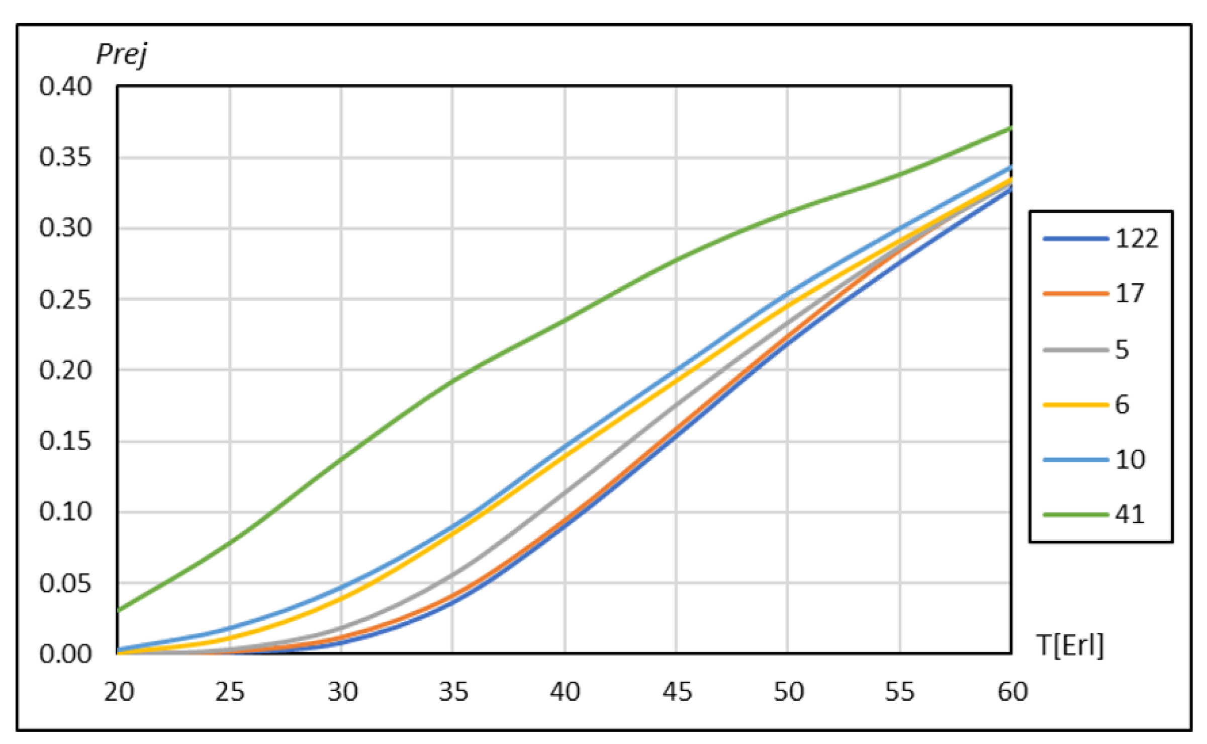
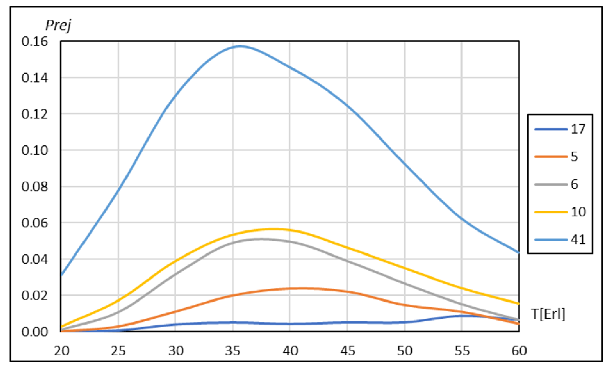
Figure 3 shows the results of the performed simulations for the chosen types of graphs placed in Table 8.

In order to better visualize the differences between the analyzed graphs, in Figure 4, the results of tests in relation to graph 122 (its value $\sigma$ is equal to 0) are shown.

As has been shown, the values of $\sigma$ decide the transmission properties of the network described with the help of graphs. Their correction, i.e., a change in the use of global transmission resources, should allow any chosen RG graph created by a specified number of nodes to possess the features of the reference graph (“best graph”). The “best graph” is such a graph whose unevenness coefficients for each edge have identical values so that the average standard deviation from the average value is zero.

Figure 5 shows examples of best graphs.

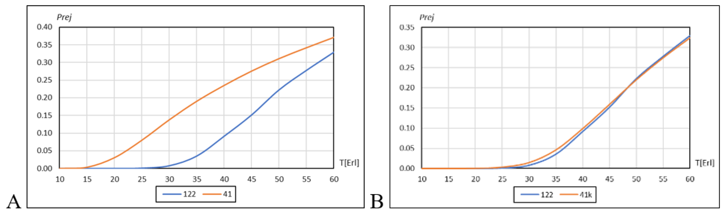
The correction procedure is illustrated using the example of graph 41 with the largest $\sigma$ coefficient value.

The following data are known: the theoretically determined mean value of the $w_{spav}=6$, the sum of all coefficients $\sum w_{spi}=108$ and their distribution (

Table 9. Distribution of $w_{spi}$.

Edge	a	b	c	d	e	f	g	h	i
${\mathit{w}}_{\mathit{spi}}$	12	5	4	5	5	4	5	5	2
Edge	j	k	l	m	n	p	q	r	s
${\mathit{w}}_{\mathit{spi}}$	8	5	12	8	8	8	5	2	5

), and the global transmission resources $RESg$ = 18 edges× 32 units = 576.

From the determined values of coefficient. the value $w_{spav}$ (

Table 10. Auxiliary Table 1.

Edge	a	b	c	d	e	f	g	h	i
$\Delta {\mathit{w}}_{\mathit{spi}}$	6	−1	−2	−1	−1	−2	−1	−1	−4
Edge	j	k	l	m	n	p	q	r	s
$\Delta {\mathit{w}}_{\mathit{spi}}$	2	−1	6	2	2	2	−1	−4	−1

) is subtracted.

The obtained values are divided by the sum of $\sum w_{spi}$ and then multiplied by the originally assumed number of resource units for each edge (

Table 11. Auxiliary Table 2.

Edge	a	b	c	d	e	f	g	h	i
$\Delta \mathit{RES}$	32.00	−5.33	−10.67	−5.33	−5.33	−10.67	−5.33	−5.33	−21.33
Edge	j	k	l	m	n	p	q	r	s
$\Delta \mathit{RES}$	10.67	−5.33	32.00	10.67	10.67	10.67	−5.33	−21.33	−5.33

).

Then, after rounding to integer values, the obtained values are added to the primary resources (

Table 12. Results of counting.

Edge	a	b	c	d	e	f	g	h	i
$\Delta \mathit{RES}$	64	27	21	27	27	21	27	27	11
Edge	j	k	l	m	n	p	q	r	s
$\Delta \mathbf{RES}$	43	27	64	43	43	43	27	11	27

).

The obtained results of tests are shown in Figure 6A before the correction and in Figure 6B after the correction.

Table 7 shows that the graphs marked 27 and 28; although they have different distributions of unevenness coefficients (

Table 13. Distributions of $w_{spi}$.

Graph	a	b	c	d	e	f	g	h	i
27	5.333	5.333	6.667	6.667	5.333	6.667	6.667	6.667	6.667
28	4.667	6.000	6.667	6.667	6.000	6.667	6.667	6.000	6.000
Graph	j	k	l	m	n	p	q	r	s
27	5.333	6.667	5.333	5.333	6.667	5.333	5.333	6.667	5.333
28	6.667	4.667	6.000	4.667	6.667	6.000	6.000	6.000	6.000

), they have the same calculated value of the standard deviation, and it amounts to $\sigma =0.6667$.

The tests performed showed that they have the same transmission properties as those shown in Figure 7.

Conclusion: Based on the analysis of the determined values of $\sigma$, it is possible to compare the transmission properties of networks described by graphs without performing simulation tests. The smaller the value of $\sigma$, the better the transmission properties of the network described by the RG graph. However, it is not a measure of these properties but merely an indicator. The analysis of the results showed that for the selected number of nodes constituting Reference Graphs of a given degree, the total number of coefficients of unevenness is strictly defined. Its exemplary values are given in

Table 14. Total values of the coefficients of $w_{spi}$ for the third-degree nodes.

Node Number	6	8	10	12	14	16	18	20	22	24	26	28	30
$\sum w_{spiN}$	42	88	150	252	378	528	702	900	1122	1416	1742	2100	2490
	D(G) = 2			D(G) = 3						D(G) = 4

and

Table 15. Total values of the $w_{spi}$ coefficients for the fourth-degree nodes.

Node Number	6	7	8	9	10	11	12	13	14	15	16	17
$\sum w_{spiN}$	36	56	80	108	140	176	216	260	308	360	416	476
	D(G) = 2
Node Number	18	19	20	21	22	23	24	25	26	27	28	29
$\sum w_{spiN}$	558	646	740	840	946	1058	1176	1300	1430	1566	1708	1856
	D(G) = 3

.

Analyzing the determined summary values $\sum w_{spiN}$ contained in the tables, it was found that they can be calculated theoretically for any Reference Graph using the following formula:

$$\sum w_{spiN}=N·(N-1)·d_{av}$$

(12)

where N is the number of nodes forming the graph and $d_{av}$ is average path length in the graph. The legitimacy of this formula can be explained as follows: each N node is connected to all other nodes through paths of a specified length; the sum of all lengths of these paths divided by the number of nodes gives the value $d_{av}$.

4. Summary and Conclusions

This paper presents some issues related to the study of transmission properties of networks whose topologies are described by Reference Graphs. In order to accomplish this goal, a simulation program was developed, and the probability of the call rejection was used as the measure for such transmission properties. As a result of the tests, it was found that despite the same basic values of parameters of Reference Graphs (that is, the diameter and the average path length), in some cases, the networks modelled by these graphs have different transmission properties. This finding became the starting point of identifying factors that could explain this phenomenon. It was assumed that the number of uses of the individual edges of the graph could be such a factor. A software tool was developed to determine this number. During the simulations, it was determined that there is an uneven use of individual edges of the graphs describing the networks. Analysis of the obtained results led to the conclusion that the effect on the occurrence of this phenomenon was due to the number of uses of specific edges in minimum length paths, specifically their presence in parallel paths. The unevenness coefficient was defined, and it can be used to distribute the network resources used by the edges to transmit information. The general conclusion that results from the presented paper is as follows: transmission properties of networks described by RG graphs depend on the distribution of the values of unevenness coefficients, and with the assistance of the analysis of their standard deviation from the theoretically determined expected value, one can choose, without resorting to simulation tests, the networks with the best transmission properties.

References

1. Kotsis, G.; Awiuni, B. Interconnection Topologies and Routing for Parallel Processing Systems (ACPC/TR 92-19); Technical Report for Austrian Center for Parallel Computation: Wien, Austria, 1996. [Google Scholar]
2. Pedersen, J.M.; Riaz, T.M.; Dubalski, B.; Madsen, O.B. A comparison of network planning strategies. In Proceedings of the 2008 10th International Conference on Advanced Communication Technology, Gangwon, Korea, 17–20 February 2008; Volume 1, pp. 702–707. [Google Scholar] [CrossRef]
3. Coffman, K.; Odlyzko, A. Growth of the Internet, Optical Fiber Telecommunicaitons IV B: Systems and Impairments, 4th ed.; Academic Press: Cambridge, MA, USA, 2002. [Google Scholar]
4. Gutierrez, J.M.; Riaz, T.; Pedersen, J.M.; Madsen, O.B. Influence of schematic network topology models over real physical networks. In Proceedings of the 2009 11th International Conference on Advanced Communication Technology, Gangwon-Do, Korea, 15–18 February 2009; Volume 1, pp. 599–604. [Google Scholar]
5. Xu, J. Topological Structure and Analysis of Interconnection Networks; Springer Science & Business Media: Boston, MA, USA, 2013; Volume 7. [Google Scholar]
6. Dehmer, M.; Moutari, S.; Emmert-Streib, F. 16. Graph theory and network analysis. In Mathematical Foundations of Data Science Using R; De Gruyter Oldenbourg: Berlin, Germany, 2020; pp. 305–330. [Google Scholar]
7. Agarwal, R.; Trivedi, R. Network Analysis and Synthesis Through Graph Theory as a Tool. J. Microw. Eng. Technol. 2019, 6, 11–17. [Google Scholar]
8. Majeed, A.; Rauf, I. Graph theory: A comprehensive survey about graph theory applications in computer science and social networks. Inventions 2020, 5, 10. [Google Scholar] [CrossRef] [Green Version]
9. Deswal, S.; Singhrova, A. Application of graph theory in communication networks. Int. J. Appl. Innov. Eng. Manag. 2012, 1, 66–70. [Google Scholar]
10. Diestel, R. Graph Theory. Graduate Texts in Mathematics, 5th ed.; Springer: Heidelberg/Berlin, Germany, 2017; Volume 173. [Google Scholar]
11. Ramaswami, R.; Sivarajan, K.; Sasaki, G. Optical Networks: A Practical Perspective, 3rd ed.; Morgan Kaufmann Publisher (Elsevier): Burlington, MA, USA, 2009. [Google Scholar]
12. Ramaswami, R.; Sivarajan, K.N. Design of logical topologies for wavelength-routed optical networks. IEEE J. Sel. Areas Commun. 1996, 14, 840–851. [Google Scholar] [CrossRef] [Green Version]
13. Lee, H. Analysis of chordal ring network. IEEE Trans. Comput. 1981, 100, 291–295. [Google Scholar]
14. Gavoille, C. A survey on interval routing. Theor. Comput. Sci. 2000, 245, 217–253. [Google Scholar] [CrossRef] [Green Version]
15. Narayanan, L.; Opatrny, J. Compact routing on chordal rings of degree 4. Algorithmica 1999, 23, 72–96. [Google Scholar] [CrossRef]
16. Bujnowski, S.; Dubalski, B.; Zabłudowski, A. Analysis of chordal rings. IEEE Trans. Comput. 2003, 100, 291–295. [Google Scholar]
17. Morillo, P.; Comellas, F.; Fiol, M. The optimization of chordal ring networks. Commun. Technol. 1987, 295–299. [Google Scholar]
18. Andrés Yebra, J.L.; Fiol Mora, M.À.; Morillo Bosch, M.P.; Alegre de Miguel, I. The diameter of undirected graphs associated to plane tessellations. Ars Comb. 1985, 20, 159–171. [Google Scholar]
19. Mehta, Y.A. Low Diameter Regular Graph as a Network Topology in Direct and Hybrid Interconnection Networks. Ph.D. Thesis, University of Illinois, Champaign, IL, USA, 2005. [Google Scholar]
20. Ledziński, D.; Marciniak, B.; Śrutek, M. Referential graphs. Telekomunikacja i Elektronika/Uniwersytet Technologiczno-Przyrodniczy w Bydgoszczy 2013, 17, 37–73. [Google Scholar]
21. Bujnowski, S.; Marciniak, T.; Lutowski, Z.; Marciniak, B.; Bujnowski, D. Modeling Telecommunication Networks with the Use of Reference Graphs. In Proceedings of the International Conference on Image Processing and Communications, Bydgoszcz, Poland, 14–16 November 2017; Springer: Cham, Switzerland, 2017; pp. 115–126. [Google Scholar]
22. Bujnowski, S.; Marciniak, T.; Marciniak, B.; Lutowski, Z. The Analysis of the Possibility to Construct Optimal Third-degree Reference Graphs. J. UCS 2020, 26, 528–546. [Google Scholar]
23. Bujnowski, S.; Marciniak, T.; Marciniak, B.; Lutowski, Z.; Marchewka, A. Analysis of the Influence of Transmission Resources Control in Tree Structure Networks. Image Process. Commun. 2018, 23, 11–19. [Google Scholar] [CrossRef] [Green Version]
24. Bujnowski, S.; Marciniak, T.; Marciniak, B.; Lutowski, Z. Impact of Resource Control in Irregular Networks on their Transmission Properties. J. UCS 2019, 25, 591–610. [Google Scholar]
25. Graham, R.L.; Knuth, D.E.; Patashnik, O.; Liu, S. Concrete mathematics: A foundation for computer science. Comput. Phys. 1989, 3, 106–107. [Google Scholar] [CrossRef]
Figure 1. Nine-node Reference Graphs.
Electronics 10 01684 g001
Figure 2. Results of simulating the probability of rejecting a call in the function of traffic density for graphs A and B (Figure 1). P r e j —probability of rejecting the call for realization, T—density of the generated traffic measured in Erlangs.
Electronics 10 01684 g002
Figure 3. Results of simulations for chosen graphs.
Electronics 10 01684 g003
Figure 4. Results of simulations in reference to graph 122.
Electronics 10 01684 g004
Figure 5. Examples of graphs with the best transmission properties (“best graphs”).
Electronics 10 01684 g005
Figure 6. Results of simulations for graph 41 compared to graph 122: (A) without the correction procedure; (B) with the correction procedure.
Electronics 10 01684 g006
Figure 7. Results of simulations: (A) without any correction; (B) with correction.
Electronics 10 01684 g007