Article

Deep Gradient Prior Regularized Robust Video Super-Resolution

1
Postdoctoral Research Center of ICBC, Beijing 100140, China
2
Center for Biomedical Image Computing and Analytics, University of Pennsylvania, Philadelphia, PA 19104, USA
*
Author to whom correspondence should be addressed.
Electronics 2021, 10(14), 1641; https://doi.org/10.3390/electronics10141641
Submission received: 16 June 2021 / Revised: 3 July 2021 / Accepted: 5 July 2021 / Published: 9 July 2021
(This article belongs to the Special Issue Circuits, Systems, and Signal Processing for Display Applications)

Abstract

:
This paper proposes a robust multi-frame video super-resolution (SR) scheme to obtain high SR performance under large upscaling factors. Although the reference low-resolution frames can provide complementary information for the high-resolution frame, an effective regularizer is required to rectify the unreliable information from the reference frames. As the high-frequency information is mostly contained in the image gradient field, we propose to learn the gradient-mapping function between the high-resolution (HR) and the low-resolution (LR) image to regularize the fusion of multiple frames. In contrast to the existing spatial-domain networks, we train a deep gradient-mapping network to learn the horizontal and vertical gradients. We found that adding the low-frequency information (mainly from the LR image) to the gradient-learning network can boost the performance of the network. A forward and backward motion field prior is used to regularize the estimation of the motion flow between frames. For robust SR reconstruction, a weighting scheme is proposed to exclude the outlier data. Visual and quantitative evaluations on benchmark datasets demonstrate that our method is superior to many state-of-the-art methods and can recover better details with less artifacts.

1. Introduction

Image/video super-resolution (SR) plays an important role in various applications such as computer vision, image recognition and high-definition display devices. The demand for high-performance SR algorithms is growing as high and ultra-high-definition displays have become prevalent. In general, video super-resolution can be divided into two categories: single image-based methods and multi-frame-based methods.
Bilinear, bicubic and spline interpolation are usually used for video super-resolution due to their low complexity. For these methods, fixed interpolation kernels are used to estimate the unknown pixels on the HR grid. However, the fixed kernel strategy will produce visually annoying artifacts such as jaggy edges, ringing effects and blurred details in the output image. Advanced interpolation methods [1,2,3,4,5] which take image structure into consideration can produce less jaggy edges. However, these methods still tend to produce blurry images, especially for large upscaling ratios. Learning-based methods try to reconstruct the high-resolution images via the mapping between the LR and HR images [6,7,8,9]. Timofte et al. [7,10] propose to replace the LR patches by the most similar dictionary atoms with pre-computed embedding matrix. Self-example approaches [11] exploit the fact that patches of similar pattern tend to recur in the image itself. More recently, deep neural networks have shown its potential to learn hierarchical representations of the high-dimensional data. Convolutional neural network (CNN)-based methods have achieved impressive results [8,12,13,14,15,16,17,18,19] in image/video SR.
Multi-frame-based super-resolution methods [20,21,22,23,24,25,26,27,28,29,30,31,32,33] use multiple images that describe the same scene to generate one HR image. They assume that different frames contain complementary information of the high-resolution frame. Thus, the key points of multiple frame SR include registration and fusion of the frames. Typical multi-frame SR methods [20,21,25,32] align the frames in sub-pixel level and reconstruct the HR frame based on the observation model. These methods perform well if the motions between the LR frames are small and global. However, it is difficult for them to handle large scale factors and large motions. Learning-based multi-frame SR methods learn a mapping directly from low-resolution frames to high-resolution frames [27,28,29]. These methods use the optical flow estimation to warp the frames according to the current frame and learn multi-frames fusion progress from the external database. Liao et al. [27] propose to handle the large and complex motion problems in multi-frame SR by deep-draft ensemble learning based on convolutional neural networks. More advanced methods learn the sub-pixel registration and the fusion function simultaneously via the deep neural networks [26,30]. However, the complex motion makes the learning of multiple fusion difficult and important image information may be eliminated by these methods.
Because of the ill-posedness of SR problems, prior models such as Total variation [34], sparse representation [35,36,37,38], steering kernel regression [39], Markov random field (MRF) [40], Non-local similarity [41,42,43] are used to regularize the estimated image. Sophisticated priors such as gradient profile prior [44,45,46] are proposed for image super-resolution. However, modeling the gradient field via simple models ignores the local geometric structures of the gradients.
In this paper, a robust multi-frame video super-resolution scheme is proposed to deal with large upscaling factors. Because of the ill-posedness of SR problem, a gradient prior learning network is trained to regularize the reconstruction of the HR image. The gradient network takes the upsampled LR image as inputs and learns the gradient prior knowledge from the external dataset. Then the learned gradient prior participates in the multi-frame fusion to predict the final HR image. Instead of directly learning the mapping from the LR gradients to HR gradients, we add the low-frequency information to the input of the network to stabilize the gradient learning and boost the performance. The HR reconstruction branch takes the LR frames as inputs, which provide the complementary information for the high-resolution frame. In the fusion stage, the learned gradients prior regularizes the reconstructed HR image to be visually nature. Experimental results demonstrate that our method is superior to many state-of-the-art single and multi-frame super-resolution methods in large upscaling factor, especially the edge and texture regions.
The contributions of the proposed scheme include:
(1) We propose a novel deep gradient-mapping network for video SR problems. The network learns the gradient prior from the external datasets and regularize the SR reconstructed image. The effectiveness of this prior is analyzed.
(2) To obtain the high-resolution motion fields, we propose to estimate the motions in the low-resolution scale and then interpolate them to the high resolution. The motion field is regularized by a forward-backward motion field prior, which brings in more accurate estimation around the motion boundary.
(3) A weighting scheme is proposed to exclude the outlier data for robust SR reconstruction.
The rest of this paper is organized as follows. Section 2 gives the background of this paper. Section 3 introduces the proposed gradient prior learning network. Section 4 studies the estimation of the motion field and the robust SR reconstruction using the reference LR frames. Experimental results are reported in Section 5 and Section 6 concludes the paper.

2. Background

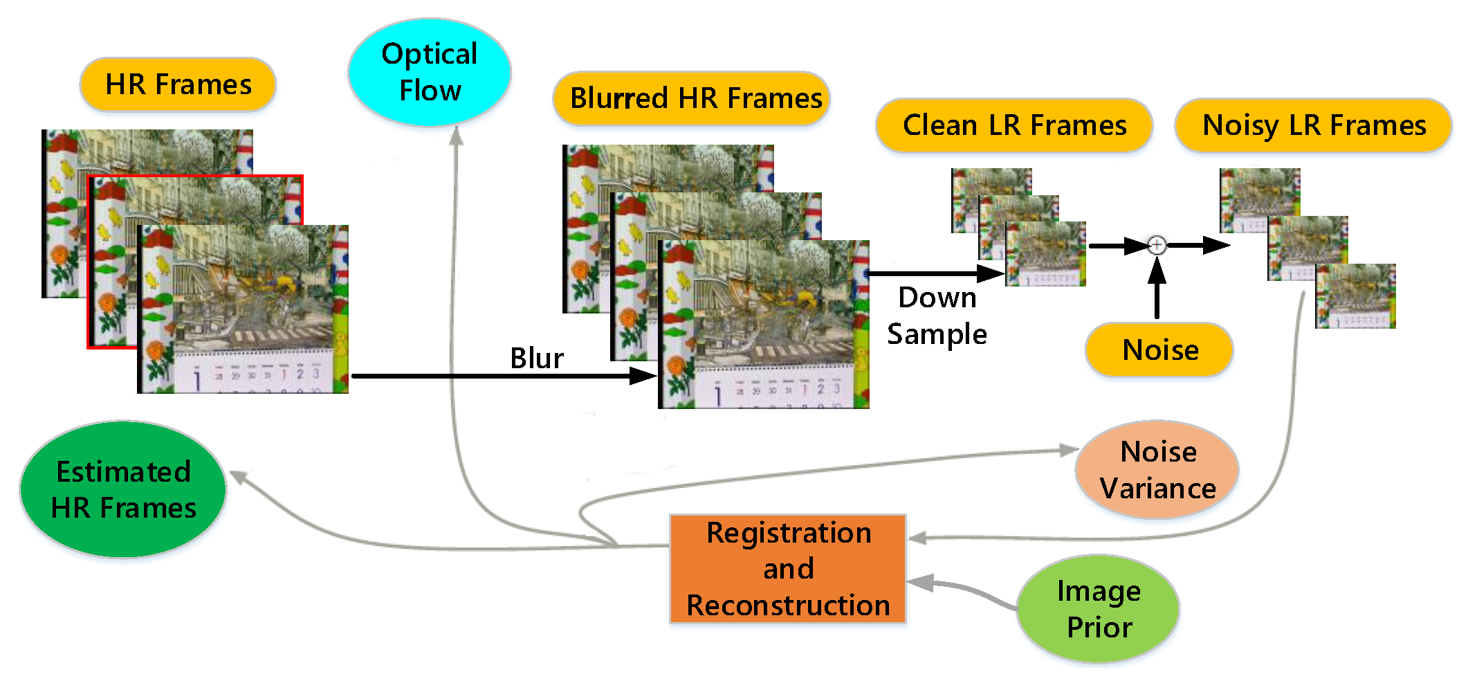
2.1. Framework of Multiple Frames SR Reconstruction

As shown in Figure 1, the degradation of video frames is usually caused by the atmospheric turbulence, inappropriate camera settings, downscaling determined by the output resolution and noise produced by the sensor. Based on some studies on camera sensor modeling, the commonly used video frames observation model describes the relationship between an HR frame and a sequence of LR frames: the LR frames are acquired from the corresponding HR frame through motion, blurring and down-sampling. In this process, the LR frames may be disturbed by noise. Thus, the video frames observation model can be formulated as follows:
y k = D · H · F u k , v k · x + n k , k = M , 0 , , M
where y k represents the k-th Low-resolution (LR) frame of size P Q × 1 . x denotes the vectorized HR frame of size s 2 P Q × 1 , where s is the down-sampling factor. 2 M + 1 is the number of LR frames. F u k , v k represents the geometric warping matrix between the HR frame and the k-th LR frame, where u k and v k represents the horizontal and vertical displacement fields, respectively. H is the blurring matrix of size s 2 P Q × s 2 P Q and D denotes the down-sampling matrix of size P Q × s 2 P Q . n k represents the additive noise of the k -th LR frame with the size of P Q × 1 . Here, we define the y 0 frame as the current LR frame and the neighboring LR frames, { y k } k 0 are the reference frames.
Assuming that the neighboring LR frames in the temporal domain describe the same HR scene and have complementary information to each other, we intend to estimate the HR frame using the LR frames. In this paper, we cast the multi-frame video super-resolution as an inverse problem. Given multiple LR frames { y k } k = 1 M , the original HR frame x can be estimated via the maximum a posterior probability (MAP) estimator:
x ^ = arg max x   k = M M log ( Pr ( y k | x ) ) + log ( Pr ( x ) ) .
where log ( Pr ( y k | x ) ) indicates the likelihood of x and log ( Pr ( x ) ) corresponds to the image prior knowledge. As Pr ( y | x ) characterizes the relationship between y k and x , the noise probability model should be established.

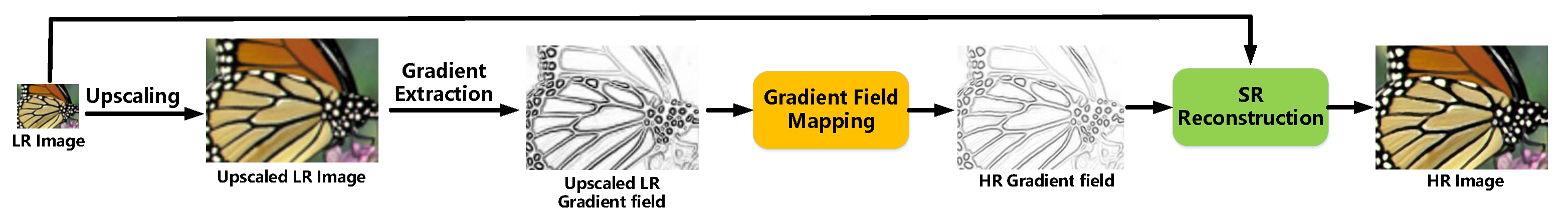
2.2. Gradient-Based Super-Resolution

During the image acquisition process, the LR images lose parts of its visual details compared with the original HR images. The lost visual details are high-frequency in nature, and is believed to be mostly contained in the image gradient field. Many approaches try to recover the high-frequency image details by modeling and estimating the image gradients.
SR framework of the gradient-based methods is illustrated in Figure 2. The LR image y is first upsampled to the high resolution using a simple interpolation method. This upsampled LR image y u usually contains visual artifacts due to the loss of high-frequency information. The lost image details such as edges and textures are mainly contained in image gradients. Therefore, the framework extracts the gradient field G y u from y u and process it by a gradient recover operation, say P ( · ) :
G ˜ x = P G y u
where G ˜ x is the estimated HR gradient field. G ˜ x is supposed to contain more accurate information about the image details. Finally, the HR image x ˜ is reconstructed by fusing the LR image y with the obtained HR gradient field G ˜ x :
x ˜ = F y   , G ˜ x
where F ( · ) is the fusion operation. For the reconstruction-based SR methods, the fusion operation F ( · ) is usually formulated as an MAP estimator (2).
Sun et al. [44] try to model the gradient-mapping function from the LR image to HR image by a statistical and parametric model. As the sharp edges in the natural image are related to the concentration of gradients perpendicular to the edge, Sun et al. [44] develop the gradient transform to convert the LR gradients to the HR gradients. However, it is rather difficult to model the gradients of an image with only a few parameters. Thus, the obtained HR images are usually over-sharped or suffer from false artifacts due to the incorrect estimation of gradients. Zhu et al. [47] propose a deformable gradient compositional model to represent the non-singular primitives as compositions of singular ones. Then they use the external gradient pattern information to predict the HR gradients. Although it is more expressive than the parametric gradient prior models, performance limitations also exist, especially in the complex detail areas.
Recently, deep neural networks showed its power in learning the representations of high-dimensional data. The convolutional neural networks (CNN) have already been used for many low-level vision applications such as denoising, super-resolution and de-rain. Dong et al. [8] first develop a three-layer neural network named SRCNN to learn the non-linear mapping between the LR image and the corresponding HR image. Later, Kim et al. [13] propose a very deep CNN with residual architecture to achieve outstanding SR performance, which can use broader contextual information with larger model capacity. Another network is also designed by Kim et al. [12], which contains recursive architectures with skip connection to boost image SR performance while only a small number of model parameters are exploited. However, these methods seldom impose any prior constraints on the recovered HR image. Yang et al. [48] introduce a deep edge guided recurrent residual (DEGREE) network to progressively perform image SR by imposing properly modeled edge priors. However, the edge priors only contain small parts of the high-frequency information and limited performance improvements are reported.
In contrast to the existing CNN-based methods, we develop an end-to-end network that learns the gradient recover operation P ( · ) and then combine it with the MAP estimator F ( · ) for multiple frames SR. An overview of the framework of the proposed method is shown in Figure 3. As illustrated, our SR framework conceptually contains the following two branches: the gradient branch learns the gradient priors and the reconstruction branch estimates the HR image by fusing multiple frames regularized by the learned gradient prior knowledge.

3. Deep Gradient Prior Learning Network

In this section, we will present the technical parts of our gradient-learning network in details. In the framework, the LR image y is first upsampled by the bicubic interpolation to the desired size y u and then extract the horizontal G y u h and vertical gradients G y u v by convolve the image by discrete gradient operator [ 1 / 2 , 0 , 1 / 2 ] and [ 1 / 2 , 0 , 1 / 2 ] T , respectively. The gradients G y u h , G y u v and the upsampled image y u are combined to be fed into the network. The network performs convolutions to the input data to estimate the HR gradients G ˜ x h , G ˜ x v . The estimated image gradients are treated as image priors to regularize the high-frequency information of the reconstructed HR image x ˜ .

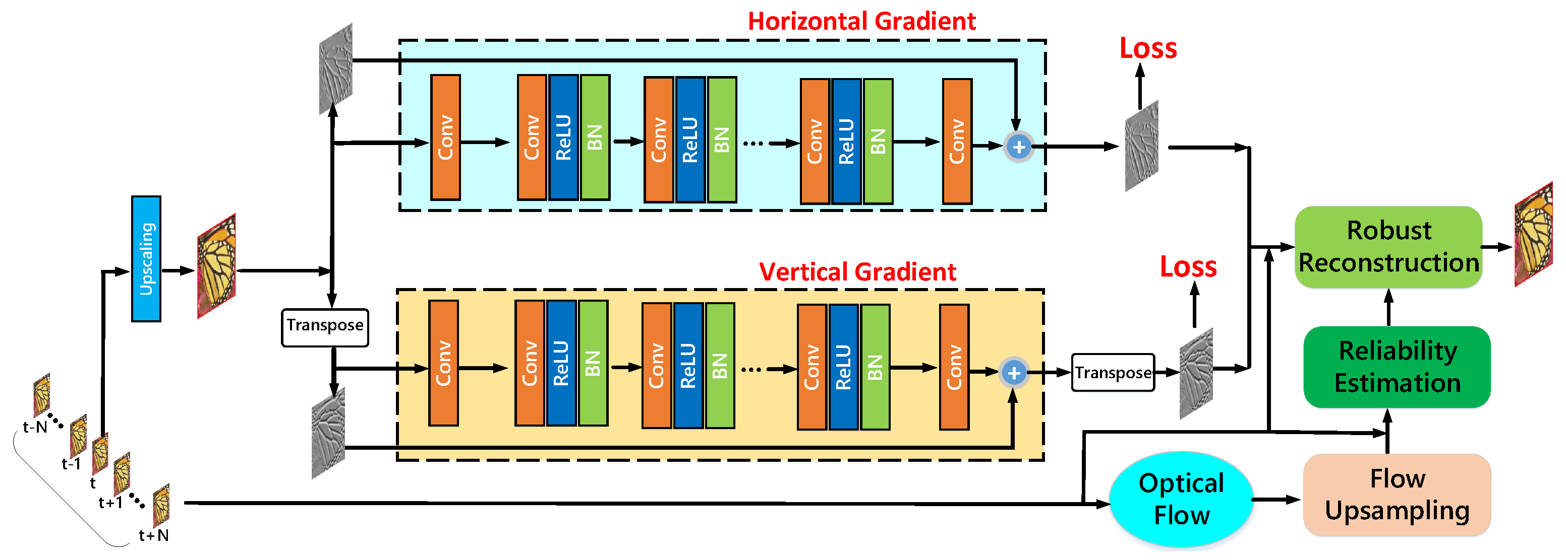
3.1. Gradient-Learning Network

As stated before, the gradient branch aims to learn the mapping:
G ˜ x h G ˜ x v = P G y u h G y u v
Due to the high-frequency nature of image gradients, P in Equation (5) is actually a high-frequency to high-frequency mapping function. During image degradation, the high-frequency components are corrupted and become more unstable compared with the low-frequency components. Thus, existing methods almost learn the low-frequency to high-frequency mapping for SR, instead. In this paper, we stabilize the learning process using the upsampled image y u . In contrast to the existing works that learn the gradient-mapping operation P ( · ) from the upsampled LR gradient G y u to the HR gradient G ˜ x , we propose to learn the mapping from the upsampled LR image to the HR gradient. Then learning of HR gradients becomes:
G ˜ x h G ˜ x v = P y u
Similar to [49,50], we could transpose the vertical gradients so that the vertical and horizontal gradients can share the weights in the training process. Learning the vertical and horizontal gradients in one network can use the correlation between the vertical and horizontal gradients.
Residual structure exhibit excellent performance in computer vision problems from the low-level to high-level tasks. As shown in Figure 2, gradients G y u h , G y u v and gradients G x h , G x v are similar in values. Thus, it is efficient to let the network learn the difference only. Then we have:
G ˜ x h G ˜ x v T = P y u + G y u h G y u v T
The gradient-learning network can be expressed as:
H 1 = W H 1 y u + B H 1 ;
H i = ReLU W H i H i 1 + B H i , 1 < i < M ;
G ˜ x h G ˜ x v T = W H M H M 1 + B H M + G y u h G y u v T
where H i is the output of the i   th layer, W H i and B H i is the filter and the bias. ReLU denotes the rectified linear unit and M denotes the final layer number. In other words, the proposed network maps the low-frequency features to the high-frequency residual features.
The proposed network has 20 convolutional layers. All the convolutional layers except the first and the last layers are followed by a ReLU layer. We simply pad zeros around the boundaries before applying convolution to keep the size of all feature maps the same as the input of each level. We add a batch norm (BN) layer after the ReLU layer. We initialize the network using the method of He et al. [51].

3.2. Training Loss Function

The final layer of the end-to-end gradient-learning network is the loss layer. Given a set of HR images { x i } and the corresponding LR images { y i } , we upsample the LR images { y i } by bicubic interpolation to obtain { y i u } and extract the horizontal and vertical gradients { G y i u h } , { G y i u v } from { y i u } . The HR gradients { G x i h } , { G x i v } are extracted from { x i } . Usually, the Mean Square Error (MSE) is adopted for training the network to guarantee high PSNR (Peak Signal to Noise Ratio) of the output HR image. As generally known, natural image gradient exhibits a heavy-tailed distribution. Thus, statistical gradient priors such as total variation (TV) adopt the Laplacian distribution and the L 1 norm in the regular term. Motivated by this, the L 1 norm is adopted for training the gradients to impose sparsity on gradients. The training process is achieved by minimizing the following total loss function:
Loss y u , G y u h , G y u v , G x h , G x v ; Θ = 1 T i = 1 T P y i u , G y i u h ; Θ G x i h 1 1 + P y i u , G y i u v ; Θ G x i v 1 1
where Θ denotes all the parameters of the network. P ( · ) denotes the gradient predictor.

3.3. Further Study of the Gradient Prior Learning Network

As shown above, one of the key points of the proposed multi-frame SR scheme is the gradient prediction branch. It regularizes the recovered high-frequency information to be closer to natural images. As gradients reveals the local variation of the image intensity, we choose to learn the mapping function from the upsampled LR image to the gradient residual of the HR image in this paper. We intend to add the reliable low-frequency information from the LR image to stabilize the learning. In this section, some experiments are conducted to support our design of this scheme.
The straight-forward strategy mentioned above is to learn the mapping function between the upsampled LR gradient and the HR gradient residual:
G ˜ x = U G y u + G y u
As shown in Figure 4, we respectively show the above-mentioned networks which are known as Scheme#1 and Scheme#2. Except for the different network input data, the network structure and the output of the networks are identical. To evaluate the learning ability of the networks, we define the gradient mean square error (GMSE) as follows to measure the horizontal and vertical gradient prediction accuracy:
GMSE h = 1 M N G ˜ h G h 2 2
GMSE v = 1 M N G ˜ v G v 2 2
where G ˜ and G denotes the predicted gradients and the groundtruth. We test the models on four commonly used test dataset and the average GMSE results are shown in Table 1. We can see that learning the gradient prior directly from the low-resolution gradients is hard for the network as only the high-frequency information is given to the network. On the contrary, learning from the intensity image itself is simpler as it can provide the low-frequency information as well.

4. Robust Super-Resolution Reconstruction from Multiple Frames

In the literature, most works modeled n k as signal independent Gaussian noise [20,32]. The Gaussian model converges to the mean estimation and is not robust to data outliers caused by the brightness inconsistency and occlusions. In this paper, we model the data errors from the reference frames as Laplacian instead. Therefore, the first term in Equation (2) can be formulated as the L 1 norm which converges to the median estimation [20]:
log ( Pr ( y k | x ) ) = 2 σ k y k D H F u k , v k x 1 1
where σ k denotes the noise / error variance. Thus, the optimization problem (2) can be generally reformulated as:
arg min x k = M M 2 σ k y k D H F u k , v k x 1 1 + λ · Y ( x ) ,
where Y ( x ) represents the regularity term and λ is the regularization parameter. In past decades, many image prior models have been proposed. The most prominent approach in this line is total variation (TV) regularization [34], which well describes the piecewise smooth structures in images. From a statistical point of view, TV is actually assuming a zero mean Laplacian distribution as the statistical model for the image gradient at all pixel locations.
However, using zero value as a mean prediction for gradients of all the pixels is misleading as natural images are typically non-stationary, especially at the edge and texture regions. Although the original HR image x is not available, we can obtain a good estimation of the gradient mean from the LR frames using the learned gradient-mapping network. Generally speaking, we want the gradient field of the reconstructed HR image is close to G ˜ . Thus, Y ( x ) here can be formulated as:
Y ( x ) = x P y 0 u p = i i x G ˜ i p
Here, i denotes the discrete gradient operator at pixel location i. G ˜ i is the expectation of the gradient at location i. In this paper, we assume that the gradients follow the non-zero mean Laplacian distribution and set p = 1 .

4.1. Displacement Estimation for the Warping Operator

One of the key problems of multi-frame video super-resolution is to construct the warping matrix F u k , v k . To obtain F u k , v k , we need to align the reference LR frames { y k } k 0 to the current HR frame x . In the literature, various motion estimation/registration techniques have been proposed. For the multi-frame video SR problem, the sub-pixel motion should be accurately estimated. Optical flow estimation concerning the dense and sub-pixel matching between frames has been studied in recent decades. However, different from the standard optical flow estimation in the same scale, we intend to estimate the motion between the LR scale and the HR scale. We can estimate the displacement between the LR and the HR image by minimizing an energy function defined as:
min u k , v k y k [ a L , b L ] D H x [ a H + u k , b H + v k ] p + β · TV ( u k , v k ) ,
where [ a L , b L ] denotes the horizontal and vertical coordinate of the LR frame and [ a H , b H ] denotes the coordinate of the HR frame. λ is a regularization parameter. The fidelity term measures the matching error between x and y k . As the above optical flow estimation between different scales is an ill-posed problem, prior knowledge of the displacement field should be imposed to regularize the flow field. Assuming the local motion consistency, the widely used TV model is used here to penalize the deviation of the flow field in the two directions while preserving the motion discontinuities. To reduce the computational cost, we here adopt a simple approximation using the interpolated flow field on the LR frames:
min u k , v k y k [ a , b ] y 0 [ a + u k , b + v k ] p + β · TV ( u k , v k )
To better deal with the outliers and occlusions, we use the L 1 norm in this paper and set p = 1 . Let [ u k f , v k f ] denotes the forward flow from y k to y 0 , [ u k b , v k b ] denotes the backward flow from y 0 to y k . We impose the prior knowledge that [ u k f , v k f ] and [ u k b , v k b ] should be the opposite. Then the objective function can be formulated as:
min u k f , v k f y k [ a , b ] y 0 [ a + u k f , b + v k f ] 1 + β · TV ( u k f , v k f ) + y 0 [ a , b ] y k [ a + u k b , b + v k b ] 1
In practice, we compute the forward and backward flow respectively and then fuse the forward and backward flow to obtain the final flow estimation:
[ u k f , v k f ] = w f · [ u k f , v k f ] w b · [ u k b , v k b ] / ( w f + w b )
where w f and w b are weight matrix with weights defined as:
w f = e div ( [ u k f , v k f ] ) 2 / h , w b = e div ( [ u k b , v k b ] ) 2 / h
div ( · ) denotes the divergence of the optical field, which measures the occlusion for each pixel. Finally, the high-resolution optical field can be obtained by interpolating the low-resolution optical field via simple interpolation methods (e.g., bicubic). Figure 5 shows the estimated optical flow fields by different schemes. We can see that the output flow field by our method is better estimated especially around the motion boundary.
Once we obtain the optical flow fields, the warping matrix can be constructed. In this paper, we use bilinear interpolation kernel to estimate the sub-pixel values of the reference HR frame x . To be concrete, the warping matrix F u k f , v k f is a sparse matrix which can be formulated as:
F u k f , v k f = ω i j ,   if   x j   is   one   of   the   four   neighbors   of   x i 0 ,   otherwise
Here j denotes the integer location of x and i is the sub-pixel location computed from the flow field u k f , v k f . The kernel weight ω i j is proportional to the distance between i and j.

4.2. Robust SR Reconstruction

Given the estimated HR gradient field G ˜ , the warping matrix F , we study how to reconstruct the HR image from the multiple LR frames in this section. The HR frame can be estimated by solving the following Bayesian-based optimization function:
arg min x 0 , σ 0 , σ k 1 2 σ 0 2 y 0 D H x 0 2 2 + λ i i x 0 G ˜ i 1 + k = M , k 0 M 2 σ k W k y k D H F k x 0 1 1 + N k = M M log σ k .
Here we assume the noise on the current frame is Gaussian noise. As described previously, the errors caused by noise, outliers and occlusions of the reference frame is modeled as Laplacian noise. We simultaneously estimate the HR frame and the noise/error variance in an overall framework. Although the L 1 norm can be robust to outliers to some extent, we add a weight matrix W k in the L 1 norm to further exclude the unreliable reference frame data in the reconstruction. W k is defined as:
W k = e ( [ u k f , v k f ] + [ u k b , v k b ] ) 2 / h · e div ( [ u k f , v k f ] ) 2 / h
Figure 6 illustrate the effectiveness of the proposed weighting strategy. It can be seen that adding W k in the framework can occlude the contribution of the outlier data in the reconstructed HR image.
To solve the optimization function (24), we use Generalized Charbonnier (GC) function ( x 2 + ϵ 2 ) α with α = 0.55 for approximation to replace the L 1 norm here. Then the objective function can be efficiently solved by alternatively updating the following function via the gradient descent algorithm:
min x 0 1 2 σ 0 2 y 0 D H x 0 2 2 + λ i i x 0 G ˜ i 2 + ϵ 2 0.55 + k = M , k 0 M 2 σ k ( W k y k D H F k x 0 ) 2 + ϵ 2 0.55 .
where ( W k y k D H F k x 0 ) 2 + ϵ 2 0.55 is pixel-wise now and the noise level:
σ k = y k D H F k x 0 2 2 / N

5. Experimental Results

In this section, experiments are conducted to evaluate the proposed method. Color RGB frames are converted to YCbCr color space and the proposed method is applied only on the luminance component. Bicubic interpolation is used for the other components. Both visual quality and quantitative quality comparisons are used for evaluation.

5.1. Experimental Settings

In our experiments, we focus on upscaling the input LR frames by factor of 4, which is usually the most challenging case in super-resolution. Two commonly used degradation models are evaluated in this paper: (1) The LR frames are generated by first applying a Gaussian kernel with standard deviation 1.4 to the original image and then down-sampling; (2) The LR frames are generated by down-sampling using the Matlab function imresize with bicubic kernel. In our implementation, the frame number M is set as 15. In other words, we fuse 30 reference LR frames with the current LR frame to reconstruct one HR frame. For the estimation of the optical flow, β is set to 0.3 and h is set as 0.18. λ is set to 0.0002. We set the maximum outer iteration number as 8 and the maximum inner iteration number as 15. ϵ is set as 0.001. In SR reconstruction process, the step size of the gradient descent algorithm is set as 0.03 to achieve good results.

5.2. Training Details

We use 91 images from Yang et al. [6] and 200 images from the training set of Berkeley Segmentation Dataset as our training data. The validation data are 19 images from Set5 and Set14. For the network training, the data augmentation is first conducted on the training dataset with (1) flipping images horizontally and vertically (2) randomly rotate image by 90, 180, and 270 rotations. Thus, eight different versions are obtained for every image. Training images are split into patches of size 48 × 48 . We use the ADAM optimizer to train our model and set β 1 = 0.9 , β 2 = 0.999 , ϵ = 10 8 . The training mini-batch size is set to 32. The learning rate is initialized as 10 4 and decreased by a factor of 10 for every 10 epochs. The proposed network is trained with the MatConvNet package on a PC with NVIDIA GTX1080Ti GPU, 64GB memory and Intel Core i7 CPU.

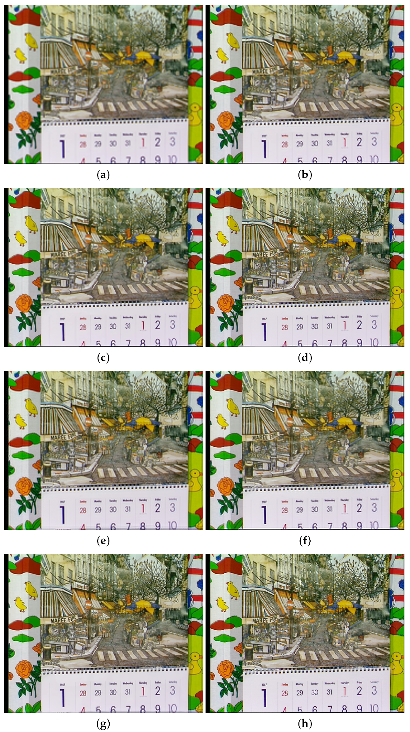
5.3. Comparisons with the State-of-the-Art Methods

In this section, both quantitative and qualitative results are given. We test our method on seven videos: calendar ( 720 × 576 ), city ( 704 × 576 ), foliage ( 720 × 480 ), walk ( 720 × 480 ), jvc009001 ( 960 × 540 ), jvc004001 ( 960 × 540 ) and AMVTG004 ( 960 × 540 ), each of which contains 31 frames. We compare our method with several recent image and video SR methods: SRCNN [8], VDSR [13], Bayesian [23], Draft [27] and LTD [29] on the seven test sequences, which include both deep learning-based methods and non-deep learning-based methods. For SRCNN [8], VDSR [13] and Draft [27], we use the models provided by the authors to generate the corresponding results, respectively. For Bayesian [23] and LTD [29], the source code is not available. The results of calendar, city, foliage and walk are downloaded from the authors’ websites. We use the re-implementation provided by Ma et al. [52] to generate the rest of the test videos for Bayesian [23]. Only the center frames (# 15) of each video sequence are reported in the paper. For fair comparison, we crop the image boundary pixels before evaluation.
In Figure 7, Figure 8, Figure 9 and Figure 10, visual results are shown to compare our SR method with other video SR methods. Details of the output HR images are given for better illustration. We can see that our method is able to produce more visually pleasant texture regions and with less artifacts around the edge regions. In Figure 7, only our method reconstructs the letters and digits clearly and with less artifacts. In Figure 9, most of the textures are smoothed out by the compared methods. In contrast, our method can reconstruct more textures. Although the outputs of the Bayesian [23] method look sharper than our method, visual artifacts of Bayesian [23] are severe. In Figure 10, better edge regions and texture regions are reconstructed by the proposed method compared with the state-of-the-art single image SR methods. The most challenging video city is shown in Figure 8. We can see that all the compared methods fail to recover the details of the building while our method can recover most of the textures.
To evaluate the quantitative quality, PSNR and SSIM are adopted here. PSNR and SSIM [53] results on the seven tested videos are respectively reported in Table 2 and Table 3, with the best results highlighted in bold. B and G refer to the bicubic kernel and Gaussian + downsample kernel, respectively. It can be seen that the proposed method achieves the highest PSNR and SSIM among the compared SR algorithms over almost all the benchmark videos. Our SR network significantly outperforms the state-of-the-art methods Bayesian [23], Draft [27] and LTD [29], especially on the video city. Specifically, for video calendar, the proposed method obtains 1.96 dB, 1.08 dB, 0.80 dB, 0.27 dB, 0.28 dB and 0.41 dB PSNR gains over bicubic, SRCNN [8], VDSR [13], Bayesian [23], Draft [27] and LTD [29]. For video city, the proposed method obtains 1.72 dB, 1.31 dB, 1.11 dB, 1.36 dB, 0.47 dB and 0.53 dB PSNR gains over bicubic, SRCNN [8], VDSR [13], Bayesian [23], Draft [27] and LTD [29]. For video jvc009001, the proposed method obtains 2.95 dB, 1.63 dB and 1.21 dB PSNR gains over bicubic, SRCNN [8], VDSR [13].

5.4. Comparisons on Running Time

In this section, the computation time of the SR algorithms are evaluated. The experiments are conducted with Matlab R2016b on a PC with Intel Core i7 3.6 GHz CPU, 16 G memory and a GTX 760Ti GPU. Our scheme mainly includes two parts: (1) motion field estimation; (2) HR image reconstruction. In Table 4, the running times of the compared SR methods on video calendar with scaling factor of 4 are listed. Please note that VDSR [13] and the gradient network of our method is running on the GPU. The rest of the compared methods and reconstruction branch of the proposed method is running on the CPU. As illustrated, the running time of the proposed method is relatively lower compared with other multi-frame video super-resolution methods. The proposed method can be implemented in C code to further accelerate its speed.

5.5. Ablation Study

The proposed SR scheme (24) in Section 4.2 contains components including learned gradient prior G ˜ i and robustness weights W k . To verify the effectiveness of the two components, we compare the proposed scheme with its variants on the 7 test videos. The comparison results are listed in Table 5. Base refers to our full baseline. Base -1 refers to Base without G ˜ i . Base -2 refers Base without W k . We can see that the full baseline achieves the best SR performance.

6. Conclusions

This paper presents a robust multi-frame video super-resolution scheme. A deep gradient-mapping network is trained to learn the horizontal and vertical gradients from the external dataset. Then the learned gradients are used to assist the reconstruction of the HR image. Instead of directly learning the mapping from the LR gradients to HR gradients, we add the low-frequency information to the input of the network to stabilize the gradient learning and boost the performance. The HR reconstruction branch takes the LR frames as input, which provide the complementary information for the high-resolution frame. In the fusion stage, the learned gradient field regularizes the reconstructed HR image to be close to nature image. Experimental results show that our method outperforms many state-of-the-art methods to a large margin on many benchmark datasets. For the future work, apart from the current frame, we could also use the reference frames to learn the HR gradients as the reference frames contain complementary information to the current frame. Furthermore, deep learning-based optical flow algorithms can be considered to better deal with the occlusion and the fast-moving scenes, which our work cannot handle very well. The code is available at https://github.com/KevinLuckyPKU/VSR.

Author Contributions

Conceptualization, Q.S. and H.L.; methodology, Q.S. and H.L.; software, Q.S.; validation, Q.S.; formal analysis, Q.S.; writing—original draft preparation, Q.S.; writing—review and editing, Q.S.; funding acquisition, Q.S. Both authors have read and agreed to the published version of the manuscript.

Funding

The APC was funded by ICBC, grant number 66105783.

Data Availability Statement

Data of our study is available upon request.

Conflicts of Interest

The authors declare no conflict of interest.

References

  1. Zhang, X.; Wu, X. Image interpolation by adaptive 2-D autoregressive modeling and soft-decision estimation. IEEE Trans. Image Process. 2008, 17, 887–896. [Google Scholar] [CrossRef] [PubMed]
  2. Li, X.; Orchard, M.T. New edge-directed interpolation. IEEE Trans. Image Process. 2000, 10, 1521–1527. [Google Scholar]
  3. Dai, S.; Mei, H.; Wei, X.; Ying, W.; Gong, Y. Soft edge smoothness prior for alpha channel super resolution. In Proceedings of the IEEE Conference on Computer Vision and Pattern Recognition, Minneapolis, MN, USA, 17–22 June 2007; pp. 1–8. [Google Scholar]
  4. Xie, J.; Feris, R.; Sun, M.T. Edge-Guided Single Depth Image Super Resolution. IEEE Trans. Image Process. 2016, 25, 428–438. [Google Scholar] [CrossRef] [PubMed]
  5. Dong, W.; Zhang, L.; Lukac, R.; Shi, G. Sparse Representation Based Image Interpolation With Nonlocal Autoregressive Modeling. IEEE Trans. Image Process. 2013, 22, 1382–1394. [Google Scholar] [CrossRef] [Green Version]
  6. Yang, J.; Wright, J.; Huang, T.S.; Ma, Y. Image Super-Resolution via Sparse Representation. IEEE Trans. Image Process. 2010, 19, 2861–2873. [Google Scholar] [CrossRef] [PubMed]
  7. Timofte, R.; Smet, V.D.; Gool, L.V. A+: Adjusted Anchored Neighborhood Regression for Fast Super-Resolution. Lect. Notes Comput. Sci. 2014, 9006, 111–126. [Google Scholar]
  8. Dong, C.; Loy, C.C.; He, K.; Tang, X. Image Super-Resolution Using Deep Convolutional Networks. IEEE Trans. Pattern Anal. Mach. Intell. 2015, 38, 295–307. [Google Scholar] [CrossRef] [PubMed] [Green Version]
  9. Freeman, W.T.; Jones, T.R.; Pasztor, E.C. Example-Based Super-Resolution. IEEE Comput. Graph. Appl. 2002, 22, 56–65. [Google Scholar] [CrossRef] [Green Version]
  10. Timofte, R.; De, V.; Van Gool, L. Anchored Neighborhood Regression for Fast Example-Based Super-Resolution. In Proceedings of the IEEE International Conference on Computer Vision, Sydney, Australia, 1–8 December 2013; pp. 1920–1927. [Google Scholar]
  11. Freedman, G.; Fattal, R. Image and video upscaling from local self-examples. ACM Trans. Graph. 2011, 30, 474–484. [Google Scholar] [CrossRef] [Green Version]
  12. Kim, J.; Lee, J.K.; Lee, K.M. Deeply-Recursive Convolutional Network for Image Super-Resolution. In Proceedings of the IEEE Conference on Computer Vision and Pattern Recognition, Las Vegas, NV, USA, 27–30 June 2016; pp. 1637–1645. [Google Scholar]
  13. Kim, J.; Lee, J.K.; Lee, K.M. Accurate Image Super-Resolution Using Very Deep Convolutional Networks. In Proceedings of the IEEE Conference on Computer Vision and Pattern Recognition, Las Vegas, NV, USA, 27–30 June 2016; pp. 1646–1654. [Google Scholar]
  14. Ledig, C.; Theis, L.; Huszar, F.; Caballero, J.; Cunningham, A.; Acosta, A.; Aitken, A.; Tejani, A.; Totz, J.; Wang, Z. Photo-Realistic Single Image Super-Resolution Using a Generative Adversarial Network. In Proceedings of the 2017 IEEE Conference on Computer Vision and Pattern Recognition (CVPR), Honolulu, HI, USA, 21–26 July 2017; pp. 105–114. [Google Scholar]
  15. Shi, W.; Caballero, J.; Huszar, F.; Totz, J.; Aitken, A.P.; Bishop, R.; Rueckert, D.; Wang, Z. Real-Time Single Image and Video Super-Resolution Using an Efficient Sub-Pixel Convolutional Neural Network. In Proceedings of the 2016 IEEE Conference on Computer Vision and Pattern Recognition (CVPR), Las Vegas, NV, USA, 27–30 June 2016; pp. 1874–1883. [Google Scholar]
  16. Zhang, K.; Zuo, W.; Gu, S.; Zhang, L. Learning Deep CNN Denoiser Prior for Image Restoration. In Proceedings of the 2017 IEEE Conference on Computer Vision and Pattern Recognition (CVPR), Honolulu, HI, USA, 21–26 July 2017; pp. 2808–2817. [Google Scholar]
  17. Donn, S.; Meeus, L.; Luong, H.Q.; Goossens, B.; Philips, W. Exploiting Reflectional and Rotational Invariance in Single Image Superresolution. In Proceedings of the IEEE Conference on Computer Vision and Pattern Recognition Workshops, Honolulu, HI, USA, 21–26 July 2017; pp. 1043–1049. [Google Scholar]
  18. Lim, B.; Son, S.; Kim, H.; Nah, S.; Lee, K.M. Enhanced Deep Residual Networks for Single Image Super-Resolution. In Proceedings of the IEEE Conference on Computer Vision and Pattern Recognition Workshops, Honolulu, HI, USA, 21–26 July 2017; pp. 1132–1140. [Google Scholar]
  19. Fan, Y.; Shi, H.; Yu, J.; Liu, D.; Han, W.; Yu, H.; Wang, Z.; Wang, X.; Huang, T.S. Balanced Two-Stage Residual Networks for Image Super-Resolution. In Proceedings of the IEEE Conference on Computer Vision and Pattern Recognition Workshops, Honolulu, HI, USA, 21–26 July 2017; pp. 1157–1164. [Google Scholar]
  20. Sina, F.; M Dirk, R.; Michael, E.; Peyman, M. Fast and robust multiframe super resolution. IEEE Trans. Image Process. 2004, 13, 1327–1344. [Google Scholar]
  21. Matan, P.; Michael, E.; Hiroyuki, T.; Peyman, M. Generalizing the nonlocal-means to super-resolution reconstruction. IEEE Trans. Image Process. 2009, 18, 36. [Google Scholar]
  22. Hiroyuki, T.; Peyman, M.; Matan, P.; Michael, E. Super-resolution without explicit subpixel motion estimation. IEEE Trans. Image Process. 2009, 18, 1958–1975. [Google Scholar]
  23. Ce, L.; Deqing, S. On Bayesian adaptive video super resolution. IEEE Trans. Pattern Anal. Mach. Intell. 2014, 36, 346–360. [Google Scholar]
  24. K?hler, T.; Huang, X.; Schebesch, F.; Aichert, A.; Maier, A.; Hornegger, J. Robust Multi-Frame Super-Resolution Employing Iteratively Re-Weighted Minimization. IEEE Trans. Comput. Imaging 2016, 2, 42–58. [Google Scholar] [CrossRef]
  25. Qiangqiang, Y.; Liangpei, Z.; Huanfeng, S.; Pingxiang, L. Adaptive multiple-frame image super-resolution based on U-curve. IEEE Trans. Image Process. 2010, 19, 3157–3170. [Google Scholar] [CrossRef]
  26. Huang, Y.; Wang, W.; Wang, L. Video Super-Resolution via Bidirectional Recurrent Convolutional Networks. IEEE Trans. Pattern Anal. Mach. Intell. 2018, 40, 1015–1028. [Google Scholar] [CrossRef] [PubMed]
  27. Liao, R.; Xin, T.; Li, R.; Ma, Z.; Jia, J. Video Super-Resolution via Deep Draft-Ensemble Learning. In Proceedings of the IEEE International Conference on Computer Vision, Santiago, Chile, 7–13 December 2015. [Google Scholar]
  28. Kappeler, A.; Yoo, S.; Dai, Q.; Katsaggelos, A.K. Video Super-Resolution with Convolutional Neural Networks. IEEE Trans. Comput. Imaging 2016, 2, 109–122. [Google Scholar] [CrossRef]
  29. Ding, L.; Wang, Z.; Fan, Y.; Liu, X.; Wang, Z.; Chang, S.; Wang, X.; Huang, T.S. Learning Temporal Dynamics for Video Super-Resolution: A Deep Learning Approach. IEEE Trans. Image Process. 2018, 27, 3432–3445. [Google Scholar]
  30. Li, D.; Wang, Z. Video Super-Resolution via Motion Compensation and Deep Residual Learning. IEEE Trans. Comput. Imaging 2017, 3, 749–762. [Google Scholar] [CrossRef]
  31. Dai, Q.; Yoo, S.; Kappeler, A.; Katsaggelos, A.K. Sparse Representation Based Multiple Frame Video Super-Resolution. IEEE Trans. Image Process. 2017, 26, 765–781. [Google Scholar] [CrossRef]
  32. Borsoi, R.A.; Costa, G.H.; Bermudez, J.C.M. A New Adaptive Video Super-Resolution Algorithm With Improved Robustness to Innovations. IEEE Trans. Image Process. 2018, 28, 673–686. [Google Scholar] [CrossRef]
  33. Liu, X.; Chen, L.; Wang, W.; Zhao, J. Robust Multi-Frame Super-Resolution Based on Spatially Weighted Half-Quadratic Estimation and Adaptive BTV Regularization. IEEE Trans. Image Process. 2018, 27, 4971–4986. [Google Scholar] [CrossRef] [PubMed]
  34. Marquina, A.; Osher, S.J. Image Super-Resolution by TV Regularization and Bregman Iteration. J. Sci. Comput. 2008, 37, 367–382. [Google Scholar] [CrossRef]
  35. Fang, L.; Li, S.; Cunefare, D.; Farsiu, S. Segmentation Based Sparse Reconstruction of Optical Coherence Tomography Images. IEEE Trans. Med Imaging 2016, 36, 407–421. [Google Scholar] [CrossRef] [Green Version]
  36. Fernandez-Granda, C.; Cands, E.J. Super-resolution via Transform-Invariant Group-Sparse Regularization. In Proceedings of the 2013 IEEE International Conference on Computer Vision, Sydney, NSW, Australia, 1–8 December 2013; pp. 3336–3343. [Google Scholar]
  37. Rida, I.; Al-Maadeed, S.; Mahmood, A.; Bouridane, A.; Bakshi, S. Palmprint Identification Using an Ensemble of Sparse Representations. IEEE Access 2018, 6, 3241–3248. [Google Scholar] [CrossRef]
  38. Rida, I.; Maadeed, N.A.; Maadeed, S.A. A Novel Efficient Classwise Sparse and Collaborative Representation for Holistic Palmprint Recognition. In Proceedings of the 2018 NASA/ESA Conference on Adaptive Hardware and Systems (AHS), Edinburgh, UK, 6–9 August 2018. [Google Scholar]
  39. Zhang, K.; Gao, X.; Tao, D.; Li, X. Single image super-resolution with non-local means and steering kernel regression. IEEE Trans. Image Process. 2012, 21, 4544–4556. [Google Scholar] [CrossRef]
  40. Freeman, W.T.; Pasztor, E.C.; Carmichael, O.T. Learning Low-Level Vision. Int. J. Comput. Vis. 2000, 40, 25–47. [Google Scholar] [CrossRef]
  41. Xiong, R.; Liu, H.; Zhang, X.; Zhang, J.; Ma, S.; Wu, F.; Gao, W. Image Denoising via Bandwise Adaptive Modeling and Regularization Exploiting Nonlocal Similarity. IEEE Trans. Image Process. 2016, 25, 5793–5805. [Google Scholar] [CrossRef]
  42. Liu, H.; Xiong, R.; Zhang, X.; Zhang, Y.; Ma, S.; Gao, W. Non-Local Gradient Sparsity Regularization for Image Restoration. IEEE Trans. Circuits Syst. Video Technol. 2016, 27, 1909–1921. [Google Scholar] [CrossRef]
  43. Zhang, J.; Xiong, R.; Zhao, C.; Zhang, Y.; Ma, S.; Gao, W. CONCOLOR: COnstrained Non-COnvex LOw-Rank Model for Image Deblocking. IEEE Trans. Image Process. 2016, 25, 1246–1259. [Google Scholar] [CrossRef]
  44. Sun, J.; Sun, J.; Xu, Z.; Shum, H.Y. Gradient profile prior and its applications in image super-resolution and enhancement. IEEE Trans. Image Process. 2011, 20, 1529–1542. [Google Scholar] [PubMed]
  45. Fattal, R. Image upsampling via imposed edge statistics. ACM Trans. Graph. 2007, 26, 95. [Google Scholar] [CrossRef]
  46. Qiang, S.; Xiong, R.; Dong, L.; Xiong, Z.; Feng, W.; Wen, G. Fast Image Super-Resolution via Local Adaptive Gradient Field Sharpening Transform. IEEE Trans. Image Process. 2018, 27, 4. [Google Scholar]
  47. Zhu, Y.; Zhang, Y.; Bonev, B.; Yuille, A.L. Modeling deformable gradient compositions for single-image super-resolution. In Proceedings of the IEEE Conference on Computer Vision and Pattern Recognition, Boston, MA, USA, 7–12 June 2015; pp. 5417–5425. [Google Scholar]
  48. Yang, W.; Feng, J.; Yang, J.; Zhao, F.; Liu, J.; Guo, Z.; Yan, S. Deep Edge Guided Recurrent Residual Learning for Image Super-Resolution. IEEE Trans. Image Process. 2017, 26, 5895–5907. [Google Scholar] [CrossRef] [PubMed] [Green Version]
  49. Zhang, J.; Pan, J.; Lai, W.S.; Lau, R.; Yang, M.H. Learning Fully Convolutional Networks for Iterative Non-blind Deconvolution. In Proceedings of the 2017 IEEE Conference on Computer Vision and Pattern Recognition (CVPR), Honolulu, HI, USA, 21–26 July 2017; pp. 6969–6977. [Google Scholar]
  50. Xu, L.; Ren, J.S.J.; Yan, Q.; Liao, R.; Jia, J. Deep edge-aware filters. In Proceedings of the International Conference on Machine Learning, Lile, France, 6–11 July 2015; pp. 1669–1678. [Google Scholar]
  51. He, K.; Zhang, X.; Ren, S.; Sun, J. Delving Deep into Rectifiers: Surpassing Human-Level Performance on ImageNet Classification. In Proceedings of the IEEE International Conference on Computer Vision, Las Vegas, NV, USA, 27–30 June 2016; pp. 1026–1034. [Google Scholar]
  52. Ma, Z.; Liao, R.; Xin, T.; Li, X.; Jia, J.; Wu, E. Handling motion blur in multi-frame super-resolution. In Proceedings of the IEEE Conference on Computer Vision and Pattern Recognition, Boston, MA, USA, 7–12 June 2015. [Google Scholar]
  53. Wang, Z.; Bovik, A.C.; Sheikh, H.R.; Simoncelli, E.P. Image quality assessment: From error visibility to structural similarity. IEEE Trans. Image Process. 2004, 13, 600–612. [Google Scholar] [CrossRef] [Green Version]
Figure 1. Observation model for multi-frame video super-resolution. The SR reconstruction is the inverse progress of video frames observation.
Electronics 10 01641 g001
Figure 2. Gradient-based super-resolution framework. A HR gradient map is estimated from the upsampled LR image and fused with the LR image to generate the final HR image.
Electronics 10 01641 g002
Figure 3. The architecture of the proposed multi-frame video SR. The framework contains two branches: the gradient prior learning branch and the HR image reconstruction branch. The gradient branch aims to predict the accurate gradient information while the image reconstruction branch fuse multiple LR frames and the gradient prior information to predict the final HR image. The motion field estimation is performed on the LR frames followed by the interpolation of the motion field to the high resolution.
Electronics 10 01641 g003
Figure 4. Analysis of two gradient-learning network. The triangle labels indicate different type of network. We use the same plain network stacked by 18 convolution+BN+ReLU layers to respectively learn different mapping function to predict the gradient image.
Electronics 10 01641 g004
Figure 5. Optical flow estimation results (color coded) of video “city”. From left to right: reference frame; Forward flow field; backward flow field and the flow field generated by the proposed method. Please enlarge the figure for better comparison.
Electronics 10 01641 g005
Figure 6. Effectiveness of the weighting strategy for occluding the unreliable reference frame data. (Left): without the weighting strategy. (Right): with the weighting strategy.
Electronics 10 01641 g006
Figure 7. Super-resolution results of “calendar” with scaling factor of x4. (a) Bicubic, (b) SRCNN [8], (c) VDSR [13], (d) Bayesian [23], (e) Draft [27], (f) LTD [29], (g) proposed method and (h) the groundtruth. Please enlarge the figure for better comparison.
Electronics 10 01641 g007
Figure 8. Super-resolution results of “city” with scaling factor of x4. (a) Bicubic, (b) SRCNN [8], (c) VDSR [13], (d) Bayesian [23], (e) Draft [27], (f) LTD [29], (g) proposed method and (h) the groundtruth. Please enlarge the figure for better comparison.
Electronics 10 01641 g008
Figure 9. Super-resolution results of “walk” with scaling factor of x4. (a) Bicubic, (b) SRCNN [8], (c) VDSR [13], (d) Bayesian [23], (e) Draft [27], (f) LTD [29], (g) proposed method and (h) the groundtruth. Please enlarge the figure for better comparison.
Electronics 10 01641 g009
Figure 10. More super-resolution results with scaling factor of x4. (a) Bicubic, (b) VDSR [13], (c) proposed method and (d) the groundtruth. Please enlarge the figure for better comparison.
Electronics 10 01641 g010
Table 1. Average GMSE results for scale x3 on benchmark datasets Set5, Set14, BSD100 and General100.
DatasetScaleBicubicScheme#1Scheme#2
Set5x347.0721.9920.04
Set14x375.1555.8254.41
BSD100x390.9173.6671.85
General100x359.5440.1638.35
Table 2. Average PSNR for scale x4 on benchmark videos calendar, city, walk, foliage, jvc009001, jvc004001 and AMVTG004.
DataBicubicSRCNN [8]VDSR [13]Draft [27]LTD [29]ProposedBayesian [23]Proposed
BBBBBBGG
calendar20.5521.4321.7122.2322.1022.5124.0824.35
city24.5724.9825.1825.8225.7626.2927.4628.82
walk26.1927.7528.1426.7928.3928.5027.8028.38
foliage23.4024.1424.3524.9424.9725.4926.1326.14
jvc00900125.4226.7427.1628.3729.34
jvc00400126.1928.2028.9429.9130.88
AMVTG00423.5724.6525.1525.5225.35
Table 3. Average SSIM for scale x4 on benchmark videos calendar, city, walk, foliage, jvc009001, jvc004001 and AMVTG004.
DataBicubicSRCNN [8]VDSR [13]Draft [27]LTD [29]ProposedBayesian [23]Proposed
BBBBBBGG
calendar0.5680.6470.6770.7100.7020.7370.8240.833
city0.5730.6150.6380.6970.6940.7350.8110.844
walk0.7960.8420.8560.7990.8570.8590.8550.864
foliage0.5630.6300.6430.7350.6960.7340.7920.776
jvc0090010.7540.8060.8280.8670.900
jvc0040010.8840.9190.9360.9460.959
AMVTG0040.5570.6210.6500.7210.734
Table 4. Average Running time (in seconds) for scale x4 on benchmark video (1 frame) calendar.
ScaleSRCNN [8]VDSR [13]Bayesian [23]DraftLTD [29]Proposed
x412.321.5 (GPU)633.912367.71163.75
Table 5. The effectiveness of different components. The PSNR values are reported.
DataBase-1Base-2Base
calendar22.3922.4222.51
city26.1825.7726.29
walk27.9425.9628.50
foliage25.3522.5625.49
jvc00900128.0428.6328.37
jvc00400129.2329.9829.91
AMVTG00425.1125.5025.52
Publisher’s Note: MDPI stays neutral with regard to jurisdictional claims in published maps and institutional affiliations.

