
A Dual-Attention Autoencoder Network for Efficient Recommendation System

Abstract
:1. Introduction
- (1)
- It utilizes the user’s attribute information and the category information of the video to reveal the potential factors of the user and the video succeedingly and combine the probability matrix factorization to realize the rating prediction.
- (2)
- It explores the role of the self-attention mechanism and multi-head self-attention mechanism in mining hidden factors of side information.
- (3)
- We have carried out numerous experiments on two public datasets. We extracted features by only using user attribute information, through item category information, through the self-attention mechanism, and through multi-head self-attention mechanism using user and item side information simultaneously to illustrate the effectiveness of the proposed MAAMF model.
2. Related Work
2.1. Matrix Factorization
2.2. Collaborative Filtering
3. Proposed MAAMF Model
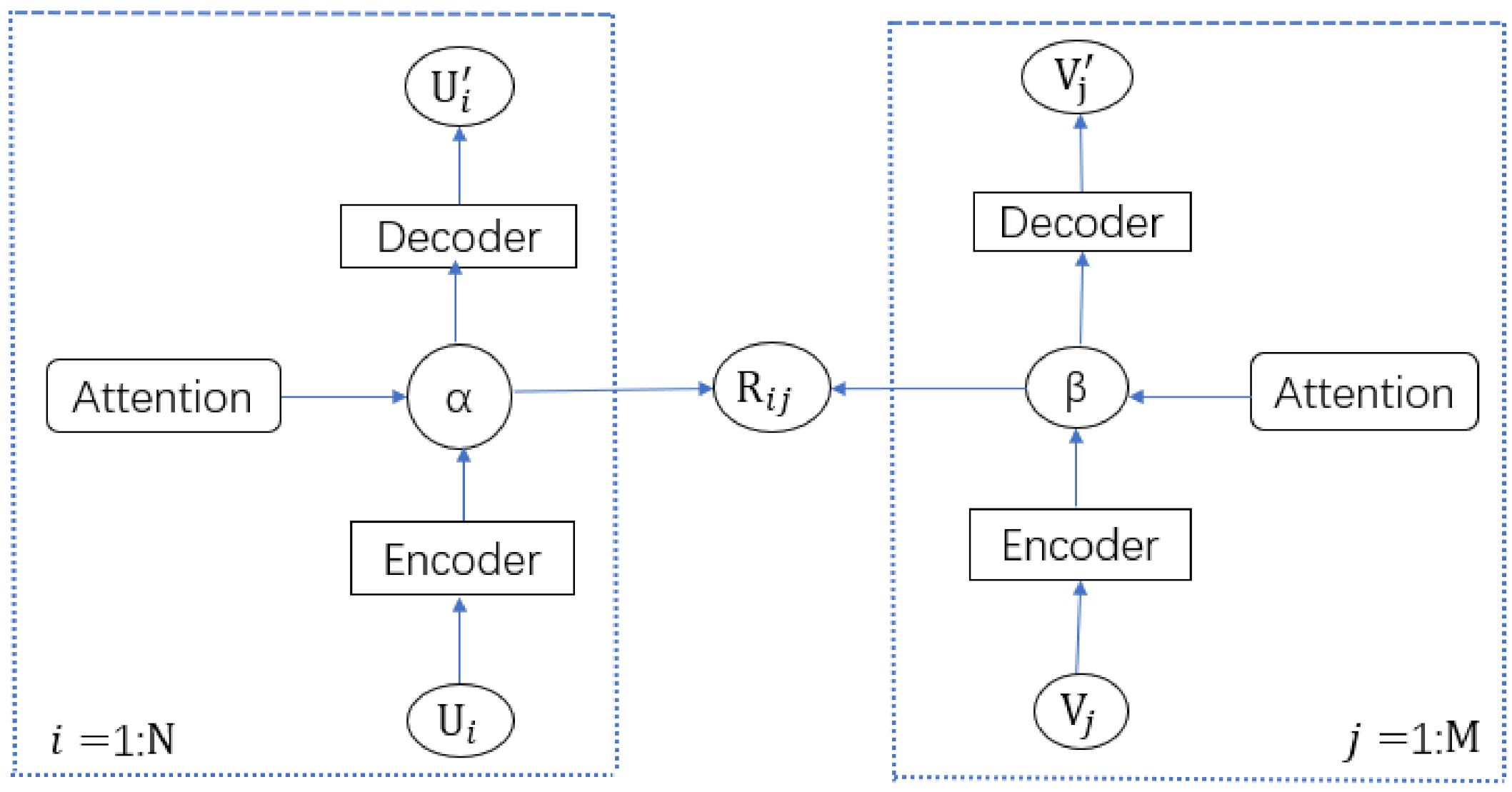
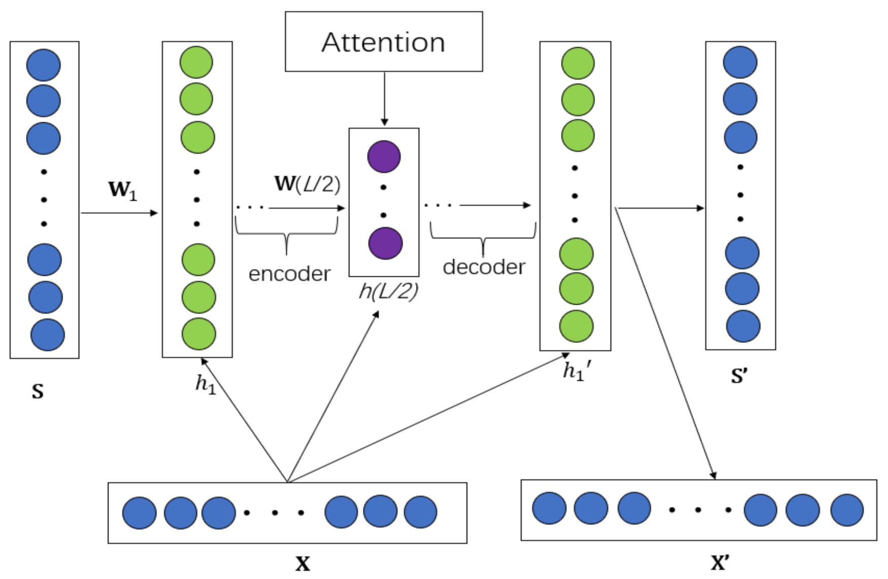
3.1. MAAMF Model Structure
3.2. MAAMF Model Principle
3.3. Model Optimization
4. Experimental Results and Discussion
4.1. Datasets and Evaluation Indicators
4.2. Experimental Software and Hardware Environment and Parameter Settings
4.3. Baseline Models
4.4. Analysis of Experimental Results
4.4.1. Influence of Balance Parameters on Experimental Results
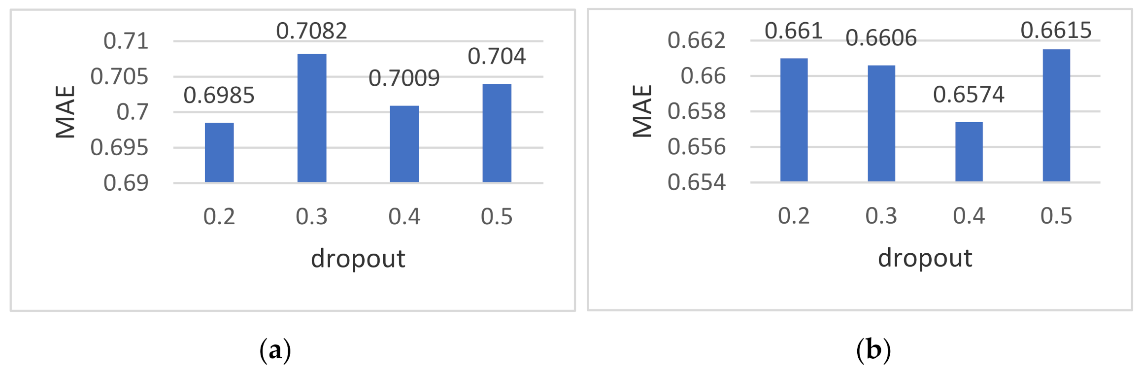
4.4.2. Influence of Different Dropouts on the Experimental Results
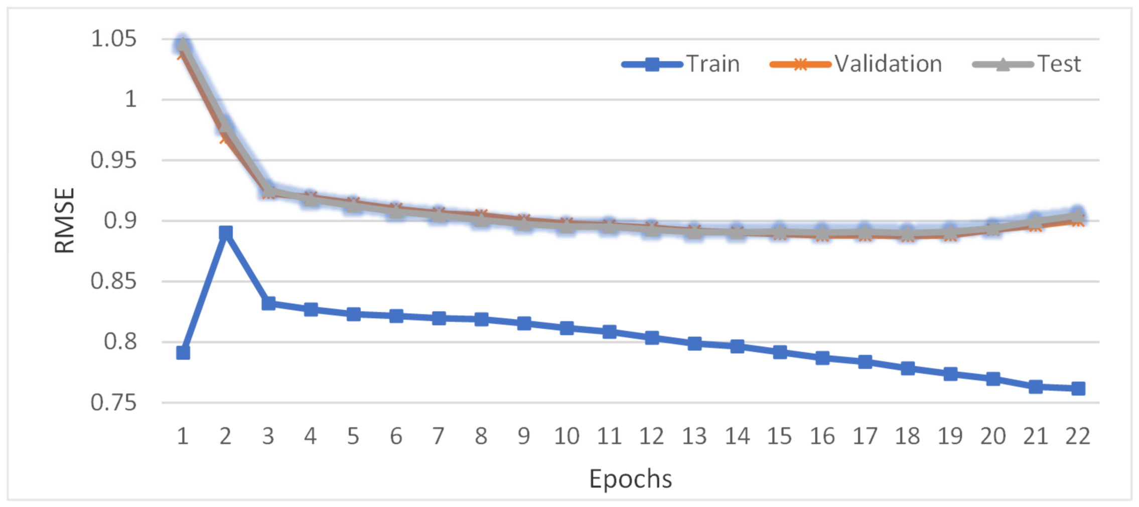
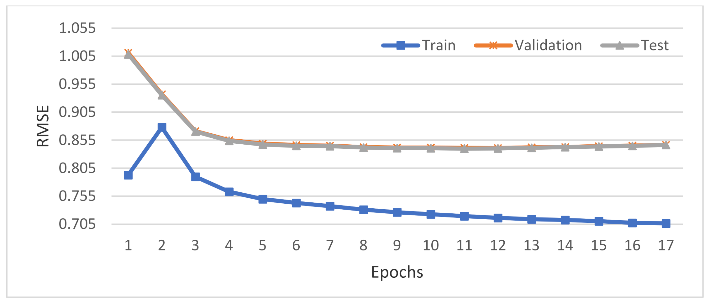
4.4.3. Changes of RMSE Value with the Number of Iterations
4.4.4. Total Results of the Experiment
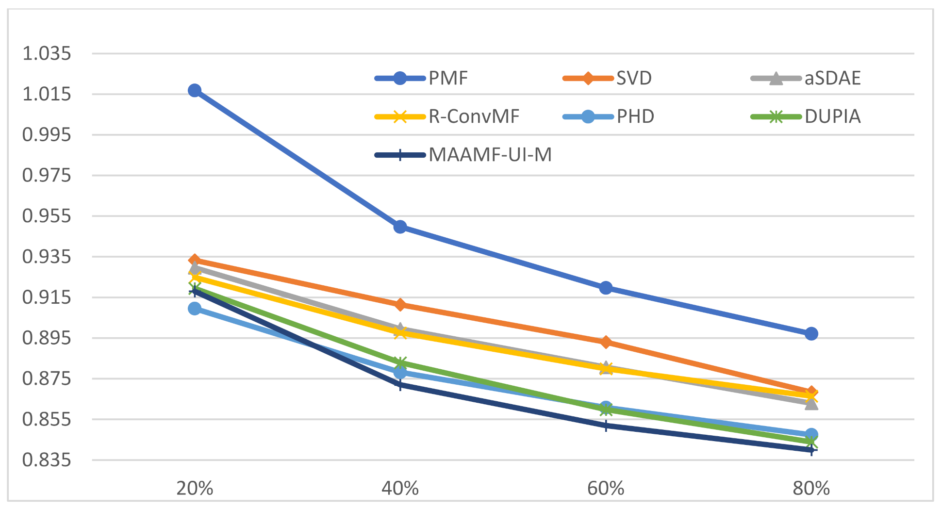
4.4.5. Comparison of Experimental Results under Different Percentages
5. Conclusions
Author Contributions
Funding
Institutional Review Board Statement
Informed Consent Statement
Data Availability Statement
Conflicts of Interest
References
- Ban, Y.; Lee, K. How the Multiplicity of Suggested Information Affects the Behavior of a User in a Recommender System. Electronics 2021, 10, 741. [Google Scholar] [CrossRef]
- Krichene, W.; Rendle, S. On Sampled Metrics for Item Recommendation. In Proceedings of the 26th ACM SIGKDD International Conference on Knowledge Discovery & Data Mining, Virtual Event, CA, USA, 6–10 July 2020; ACM: New York, NY, USA, 2020; pp. 1748–1757. [Google Scholar] [CrossRef]
- Lin, Y.; Feng, S.; Zeng, W.; Lin, F.; Liu, Y.; Wu, P. Adaptive course recommendation in MOOCs. Knowl. Based Syst. 2021, 224, 107085. [Google Scholar] [CrossRef]
- Jin, J.; Qin, J.; Fang, Y.; Du, K.; Zhang, W.; Yu, Y.; Zhang, Z.; Smola, A.J. An Efficient Neighborhood-based Interaction Model for Recommendation on Heterogeneous Graph. In Proceedings of the 26th ACM SIGKDD International Conference on Knowledge Discovery & Data Mining, Virtual Event, CA, USA, 6–10 July 2020; ACM: New York, NY, USA, 2020; pp. 75–84. [Google Scholar] [CrossRef]
- Paul, D.J.; Kundu, S. A survey of music recommendation systems with a proposed music recommendation system. In Emerging Technology in Modelling and Graphics. Advances in Intelligent Systems and Computing; Springer: New York, NY, USA, 2020; Volume 937. [Google Scholar] [CrossRef]
- Li, Z.; Liu, H.; Zhang, Z.; Liu, T.; Xiong, N.N. Learning Knowledge Graph Embedding with Heterogeneous Relation Attention Networks. IEEE Trans. Neural Netw. Learn. Syst. 2021, 10, 1–13. [Google Scholar]
- Warren, J. Big Data: Principles and Best Practices of Scalable Realtime Data Systems; Manning Publications: Shelter Island, NY, USA, 2015. [Google Scholar]
- Adomavicius, G.; Tuzhilin, A. Toward the next generation of recommender systems: A survey of the state-of-the-art and possible extensions. IEEE Trans. Knowl. Data Eng. 2005, 17, 734–749. [Google Scholar] [CrossRef]
- Li, D.; Liu, H.; Zhang, Z.; Lin, K.; Fang, S.; Li, Z.; Xiong, N.N. CARM: Confidence-aware recommender model via review representation learning and historical rating behavior in the online platforms. Neurocomputing 2021, 455, 283–296. [Google Scholar] [CrossRef]
- Liu, T.; Li, Y.; Liu, H.; Zhang, Z.; Liu, S. RISIR: Rapid Infrared Spectral Imaging Restoration Model for Industrial Material Detection in Intelligent Video Systems. IEEE Trans. Ind. Inf. 2019, 1. [Google Scholar] [CrossRef]
- Liu, T.; Liu, H.; Li, Y.; Zhang, Z.; Liu, S. Efficient Blind Signal Reconstruction with Wavelet Transforms Regularization for Educational Robot Infrared Vision Sensing. IEEE/ASME Trans. Mechatron 2019, 24, 384–394. [Google Scholar] [CrossRef]
- Sun, Z.; Guo, Q.; Yang, J.; Fang, H.; Guo, G.; Zhang, J.; Burke, R. Research commentary on recommendations with side information: A survey and research directions. Electron. Commer. Res. Appl. 2019, 37, 100879. [Google Scholar] [CrossRef] [Green Version]
- Ravanifard, R.; Buntine, W.; Mirzaei, A. Recommending content using side information. Appl. Intell. 2021, 51, 3353–3374. [Google Scholar] [CrossRef]
- Liu, T.; Wang, Z.; Tang, J.; Yang, S.; Huang, G.Y.; Liu, Z. Recommender systems with heterogeneous side information. In Proceedings of the World Wide Web Conference (WWW ’19), San Francisco, CA, USA, 13–17 May 2019; pp. 3027–3033. [Google Scholar]
- Zhang, S.; Yao, L.; Sun, A.; Tay, Y. Deep Learning Based recommender system: A survey and new perspectives. ACM Comput. Surv. 2019, 52, 1–38. [Google Scholar] [CrossRef] [Green Version]
- Batmaz, Z.; Yurekli, A.; Bilge, A.; Kaleli, C. A review on deep learning for recommender systems: Challenges and remedies. Artif. Intell. Rev. 2019, 52, 1–37. [Google Scholar] [CrossRef]
- LeCun, Y.; Bengio, Y.; Hinton, G. Deep learning. Nature 2015, 521, 436–444. [Google Scholar] [CrossRef]
- Zhang, G.; Liu, Y.; Jin, X. A survey of autoencoder-based recommender systems. Front. Comput. Sci. 2020, 14, 430–450. [Google Scholar] [CrossRef]
- Cheng, H.T.; Koc, L.; Harmsen, J.; Shaked, T.; Chandra, T.; Aradhye, H.; Anderson, G.; Corrado, G.; Chai, W.; Ispit, M.; et al. Wide & Deep Learning for Recommender Systems. In Proceedings of the 1st Workshop on Deep Learning for Recommender Systems, Boston, MA, USA, 15 September 2016; ACM: New York, NY, USA, 2016; pp. 7–10. [Google Scholar]
- Sedhain, S.; Menon, A.K.; Sanner, S.; Xie, L. AutoRec: Autoencoders meet collaborative filtering. In Proceedings of the 24th international conference on World Wide Web, Florence, Italy, 18–22 May 2015; pp. 111–112. [Google Scholar]
- Chen, S.; Wu, M. Attention collaborative autoencoder for explicit recommender systems. Electronics 2020, 9, 1716. [Google Scholar] [CrossRef]
- Kang, W.C.; Mcauley, J. Self-attentive sequential recommendation. In Proceedings of the 2018 IEEE Conference on Data Mining (ICDM), Singapore, 17–20 November 2018; IEEE: Piscataway, NJ, USA, 2018; pp. 197–206. [Google Scholar]
- Tal, O.; Liu, Y.; Huang, J.; Yu, X.; Aljbawi, B. Neural Attention Frameworks for Explainable Recommendation. IEEE Trans. Knowl. Data Eng. 2021, 33, 2137–2150. [Google Scholar] [CrossRef]
- Koren, Y.; Bell, R.; Volinsky, C. Matrix factorization techniques for recommender systems. Computer 2009, 42, 30–37. [Google Scholar] [CrossRef]
- Sarwar, B.; Karypis, G.; Konstan, J.; Riedl, J. Application of dimensionality reduction in recommender system—A case study. In Proceedings of the WebKDD-2000 Workshop, Boston, MA, USA, 20 August 2000. [Google Scholar]
- Lee, D.D.; Seung, H.S. Learning the parts of objects by non-negative matrix factorization. Nature 1999, 401, 788–791. [Google Scholar] [CrossRef]
- Nikolakopoulos, A.N.; Kalantzis, V.; Gallopoulos, E.; Garofalakis, J.D. Eigenrec: Generalizing puresvd for effective and efficient top-n recommendations. Knowl. Inf. Syst. 2018, 58, 59–81. [Google Scholar] [CrossRef] [Green Version]
- Koutrika, G. Modern recommender systems: From computing matrices to thinking with neurons. In Proceedings of the International Conference on Management of Data, Houston, TX, USA, 10–15 June 2018; pp. 1651–1654. [Google Scholar]
- Shen, X.; Yi, B.; Liu, H.; Zhang, W.; Zhang, Z.; Liu, S.; Xiong, N. Deep variational matrix factorization with knowledge embedding for recommendation system. IEEE Trans. Knowl. Data Eng. 2021, 33, 1906–1918. [Google Scholar] [CrossRef]
- Yi, B.; Shen, X.; Liu, H.; Zhang, Z.; Zhang, W.; Liu, S.; Xiong, N. Deep matrix factorization with implicit feedback embedding for recommendation system. IEEE Trans. Knowl. Data Eng. 2019, 15, 4591–4601. [Google Scholar] [CrossRef]
- Liu, T.; Liu, H.; Li, Y.; Chen, Z.; Zhang, Z.; Liu, S. Flexible FTIR Spectral Imaging Enhancement for Industrial Robot Infrared Vision Sensing. IEEE Trans. Ind. Inf. 2020, 16, 544–554. [Google Scholar] [CrossRef]
- Kim, D.; Park, C.; Oh, J.; Lee, S.; Yu, H. Convolutional matrix factorization for document context-aware recommendation. In Proceedings of the 10th ACM Conference on Recommender Systems, Boston, MA, USA, 15–19 September 2016; ACM: New York, NY, USA, 2016; pp. 233–240. [Google Scholar]
- Zheng, L.; Noroozi, V.; Yu, P.S. Joint deep modeling of users and items using reviews for recommendation. In Proceedings of the Tenth ACM International Conference on Web Search and Data Mining, Cambridge, UK, 6–10 February 2017; ACM: New York, NY, USA, 2017; pp. 425–434. [Google Scholar]
- Seo, S.; Huang, J.; Yang, H.; Liu, Y. Interpretable convolutional neural networks with dual local and global attention for review rating prediction. In Proceedings of the Eleventh ACM Conference, Como, Italy, 27–31 August 2017; ACM: New York, NY, USA, 2017; pp. 297–305. [Google Scholar]
- Wu, L.; Quan, C.; Li, C.; Wang, Q.; Zheng, B. A context-aware user-item representation learning for item recommendation. IEEE Trans. Knowl. Data Eng. 2017, 37, 1–29. [Google Scholar] [CrossRef] [Green Version]
- Chin, J.Y.; Zhao, K.; Joty, S.; Cong, G. ANR: Aspect-based neural recommender. In Proceedings of the 27th ACM International Conference on Information and Knowledge Management, CIKM, Torino, Italy, 22–26 October 2018; ACM: New York, NY, USA, 2018; pp. 147–156. [Google Scholar]
- Liu, D.; Li, J.; Du, B.; Chang, J.; Gao, R. DAML: Dual Attention Mutual Learning between Ratings and Reviews for Item Recommendation. In Proceedings of the 25th ACM SIGKDD International Conference on Knowledge Discovery & Data Mining, Anchorage, AK, USA, 4–8 August 2019; ACM: New York, NY, USA, 2019; pp. 344–352. [Google Scholar]
- Chong, C.; Min, Z.; Liu, Y.; Ma, S. Neural attentional rating regression with review-level explanations. In Proceedings of the 2018 World Wide Web Conference, Lyon, France, 23–27 April 2018; pp. 1583–1592. [Google Scholar]
- Lu, Y.; Dong, R.; Smyth, B. Coevolutionary recommendation model: Mutual learning between ratings and reviews. In Proceedings of the 2018 World Wide Web Conference, Lyon, France, 23–27 April 2018; pp. 773–782. [Google Scholar]
- Yi, T.; Luu, A.T.; Hui, S.C. Multi-pointer co-attention networks for recommendation. In Proceedings of the 24th ACM SIGKDD International Conference, London, UK, 19–23 August 2018; ACM: New York, NY, USA, 2018; pp. 2309–2318. [Google Scholar]
- Huang, X.; Liao, G.; Xiong, N.; Vasilakos, A.; Lan, T. A survey of context-aware recommendation schemes in event-based social networks. Electronics 2020, 9, 1583. [Google Scholar] [CrossRef]
- Guo, G.; Zhang, J.; Yorke-Smith, N. TrustSVD: Collaborative filtering with both the explicit and implicit influence of user trust and of item ratings. In Proceedings of the Twenty-Ninth AAAI Conference on Artificial Intelligence, Austin, TX, USA, 25–30 January 2015; pp. 123–129. [Google Scholar]
- Zhu, Z.; Wang, J. James Caverlee. In Improving top-K recommendation via joint collaborative autoencoders. In Proceedings of the 30th International Conference on World Wide Web, San Francisco, CA, USA, 13–17 May 2019; pp. 3482–3483. [Google Scholar]
- Park, C.; Kim, D.H.; Oh, J.; Yu, H. TRecSo: Enhancing top-k recommendation with social information. In Proceedings of the WWW (Companion Volume), Montréal, QC, Canada, 11–15 April 2016; pp. 89–90. [Google Scholar]
- Chen, C.; Zheng, X.; Yan, W.; Hong, F.; Zhen, L. Context-ware collaborative topic regression with social matrix factorization for recommender systems. In Proceedings of the Twenty-Eighth AAAI Conference on Artificial Intelligence (AAAI-14), Québec City, QC, Canada, 27–31 July 2014; AAAI Press: Palo Alto, CA, USA, 2014; pp. 9–15. [Google Scholar]
- Anastasiu, D.C.; Christakopoulou, E.; Smith, S.; Sharma, M.; Karypis, G. Big Data and Recommender Systems. 2016. Available online: https://conservancy.umn.edu/handle/11299/215998 (accessed on 2 June 2021).
- Sardianos, C.; Tsirakis, N.; Varlamis, I. A Survey on the Scalability of Recommender Systems for Social Networks; Springer: Cham, Switzerland, 2018. [Google Scholar] [CrossRef]
- Eirinaki, M.; Gao, J.; Varlamis, I.; Tserpes, K. Recommender Systems for Large-Scale Social Networks: A review of challenges and solutions. Future Gener. Comput. Syst. FGCS 2018, 78, 413–418. [Google Scholar] [CrossRef]
- Zhu, N.; Cao, J.; Lu, X.; Gu, Q. Leveraging pointwise prediction with learning to rank for top-N recommendation. World Wide Web 2021, 24, 375–396. [Google Scholar] [CrossRef]
- Liu, H.; Fang, S.; Zhang, Z.; Li, D.; Lin, K.; Wang, J. MFDNet: Collaborative Poses Perception and Matrix Fisher Distribution for Head Pose Estimation. IEEE Trans. Multimed. 2021, 1. [Google Scholar] [CrossRef]
- Zhao, Z.; Chi, E.; Hong, L.; Chen, J.; Nath, A.; Andrews, S.; Kumthekar, A.; Sathiamoorthy, M.; Yi, X.; Chi, E. Recommending what video to watch next: A multitask ranking system. In Proceedings of the 13th ACM Conference, Copenhagen, Denmark, 16–20 September 2019; ACM: New York, NY, USA, 2019; pp. 43–51. [Google Scholar]
- Chen, L.; Yuan, Y.; Yang, J.; Zahir, A. Improving the prediction quality in memory-based collaborative filtering using categorical features. Electronics 2021, 10, 214. [Google Scholar] [CrossRef]
- Zhang, Z.; Li, Z.; Liu, H.; Xiong, N.N. Multi-scale Dynamic Convolutional Network for Knowledge Graph Embedding. IEEE Trans. Knowl. Data Eng. 2021, 1–10. [Google Scholar] [CrossRef]
- Li, Z.; Liu, H.; Zhang, Z.; Liu, T.; Shu, J. Recalibration Convolutional Networks for Learning Interaction Knowledge Graph Embedding. Neurocomputing 2021, 427, 118–130. [Google Scholar] [CrossRef]
- Vaswani, A.; Shazeer, N.; Parmar, N. Attention is all you need. In Proceedings of the Neural Information Processing Systems 30: Annual Conference on Neural Information Processing Systems, Long Beach, CA, USA, 4–9 December 2017; pp. 5998–6008. [Google Scholar]
- Harper, F.M.; Konstan, J.A. The MovieLens datasets: History and context. ACM Trans. Interact. Intell. Syst. 2016, 5, 1–19. [Google Scholar] [CrossRef]
- Dong, X.; Yu, L.; Wu, Z. A hybrid collaborative filtering model with deep structure for recommender systems. In AAAI; AAAI Press: San Francisco, CA, USA, 2017; pp. 1309–1315. [Google Scholar]
- Kim, D.; Park, C.; Oh, J.; Yu, H. Deep hybrid recommender systems via exploiting document context and statistics of items. Inf. Sci. 2017, 417, 72–87. [Google Scholar] [CrossRef]
- Liu, J.; Wang, D.; Ding, Y. PHD: A probabilistic model of hybrid deep collaborative filtering for recommender systems. In Proceedings of the Asian Conference on Machine Learning, Seoul, Korea, 15–17 November 2017; PMLR: Seoul, Korea; Volume 77, pp. 224–239. [Google Scholar]
- Xz, A.; Hl, A.; Xc, B.; Zhong, J.; Wang, D. A novel hybrid deep recommendation system to differentiate user’s preference and item’s attractiveness. Inf. Sci. 2020, 519, 306–316. [Google Scholar]


| Notation | Meaning | Notation | Meaning |
|---|---|---|---|
| U | User side information | ϵj | Influence of Gaussian noise |
| V | Item side information | X | Side information |
| U’ | approximate representation of U | S’ | Unzipped secondary information |
| V’ | approximate representation of V | X’ | Unzipped rating information |
| W | Weight | h | Hidden layer |
| N | Number of users | L | Number of hidden layers |
| M | Number of items | h1 | First hidden layer |
| R | User item rating matrix | W1 | First layer of weight parameters |
| Ui | Side information of the i-th user | Times | |
| Vj | Side information of the j-th item | Query | |
| α | Compressed representation of Ui | Key | |
| β | Compressed representation of Vj | Values | |
| λu | User regularization parameter | parameter matrix of in the | |
| λv | Item regularization parameter | transformation |
| Dataset | User side Information | Video Side Information | User Number | Video Number | Ratings |
|---|---|---|---|---|---|
| ML-100K | ID/gender/age/job/zipcode | Video category information | 943 | 1546 | 94,808 |
| ML-1m | ID/gender/age/job/zipcode | Video category information | 6040 | 3544 | 993,482 |
| ML-100k | |||||
|---|---|---|---|---|---|
| λu | 1 | 5 | 8 | 10 | 10 |
| λv | 100 | 50 | 50 | 50 | 60 |
| RMSE | 0.9320 | 0.9050 | 0.8900 | 0.9043 | 0.9051 |
| MAE | 0.7280 | 0.7095 | 0.6985 | 0.7095 | 0.7101 |
| ML-1m | |||||
|---|---|---|---|---|---|
| λu | 1 | 3 | 3 | 3 | 5 |
| λv | 100 | 100 | 150 | 120 | 120 |
| RMSE | 0.8697 | 0.8434 | 0.8416 | 0.8399 | 0.8429 |
| MAE | 0.6787 | 0.6594 | 0.6599 | 0.6574 | 0.6601 |
| Models | Datasets | |
|---|---|---|
| ML-100k | ML-1m | |
| PMF | 0.9412 | 0.8971 |
| SVD | 0.9453 | 0.8684 |
| aSDAE | 0.9441 | 0.8723 |
| R-ConvMF | 0.9447 | 0.8470 |
| PHD | 0.9296 | 0.8465 |
| DUPIA | 0.9138 | 0.8439 |
| MAAMF-U | 0.9167 | 0.8544 |
| MAAMF-I | 0.9053 | 0.8509 |
| MAAMF-UI-S | 0.8822 | 0.8412 |
| MAAMF-UI-M | 0.8900 | 0.8399 |
| Models | 20% | 30% | 40% | 50% | 60% | 70% | 80% | t | sig |
|---|---|---|---|---|---|---|---|---|---|
| DUPIA | 0.9195 | 0.8968 | 0.8829 | 0.8694 | 0.8598 | 0.8470 | 0.8439 | 3.7520 | 0.0047 |
| MAAMF-UI-M | 0.9180 | 0.8848 | 0.8720 | 0.8589 | 0.8519 | 0.8466 | 0.8399 |
Publisher’s Note: MDPI stays neutral with regard to jurisdictional claims in published maps and institutional affiliations. |
© 2021 by the authors. Licensee MDPI, Basel, Switzerland. This article is an open access article distributed under the terms and conditions of the Creative Commons Attribution (CC BY) license (https://creativecommons.org/licenses/by/4.0/).
Share and Cite
Duan, C.; Sun, J.; Li, K.; Li, Q. A Dual-Attention Autoencoder Network for Efficient Recommendation System. Electronics 2021, 10, 1581. https://doi.org/10.3390/electronics10131581
Duan C, Sun J, Li K, Li Q. A Dual-Attention Autoencoder Network for Efficient Recommendation System. Electronics. 2021; 10(13):1581. https://doi.org/10.3390/electronics10131581
Chicago/Turabian StyleDuan, Chao, Jianwen Sun, Kaiqi Li, and Qing Li. 2021. "A Dual-Attention Autoencoder Network for Efficient Recommendation System" Electronics 10, no. 13: 1581. https://doi.org/10.3390/electronics10131581
APA StyleDuan, C., Sun, J., Li, K., & Li, Q. (2021). A Dual-Attention Autoencoder Network for Efficient Recommendation System. Electronics, 10(13), 1581. https://doi.org/10.3390/electronics10131581