
Bone Metastasis Detection in the Chest and Pelvis from a Whole-Body Bone Scan Using Deep Learning and a Small Dataset

 ,
, 
Abstract
:1. Introduction
2. Materials and Methods
2.1. Materials
2.2. Difficulties in Bone Metastasis Detection
2.3. Image Preprocessing and Normalization
2.3.1. Spatial Normalization
2.3.2. Intensity Normalization
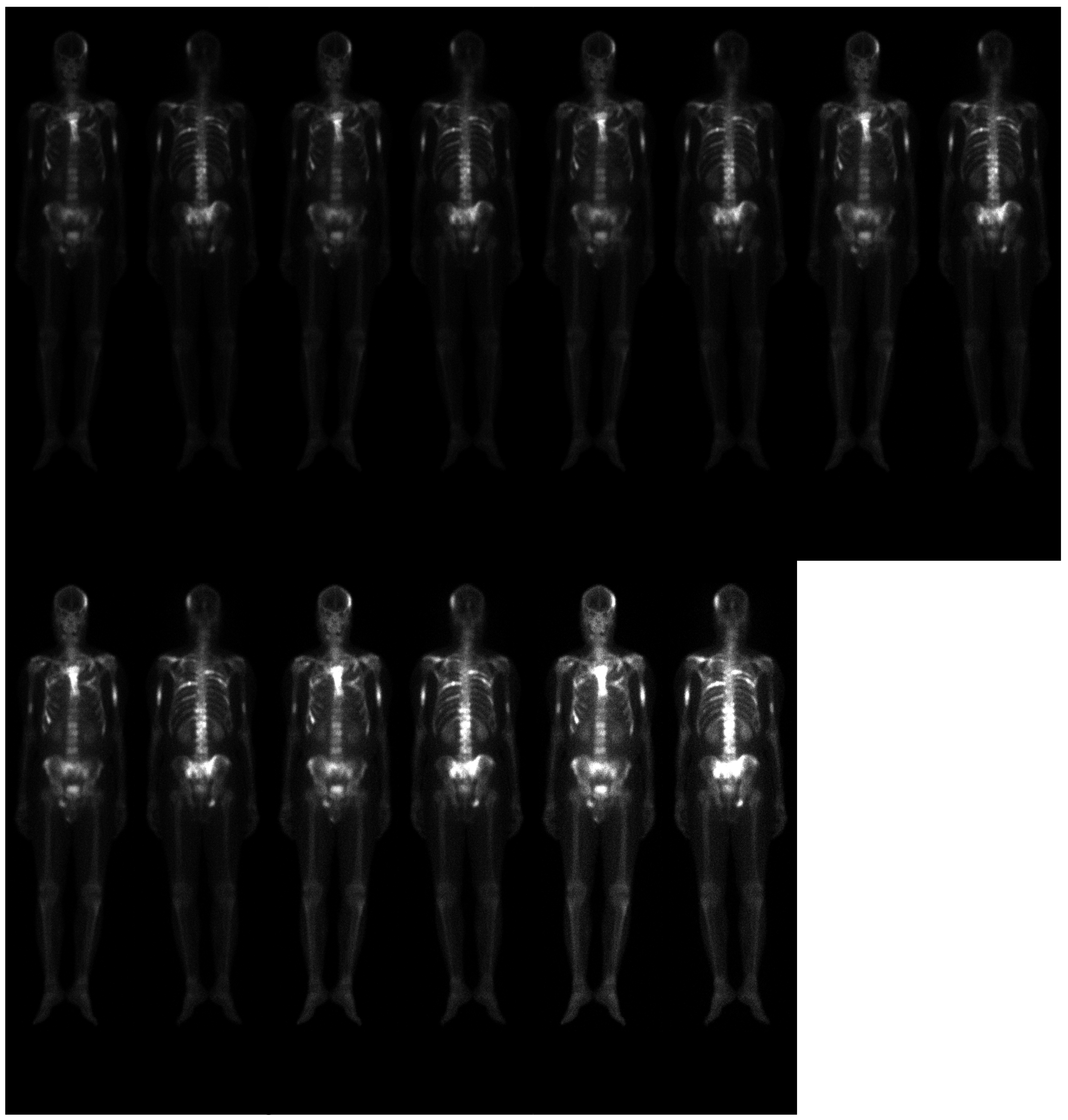
2.3.3. Data Augmentation
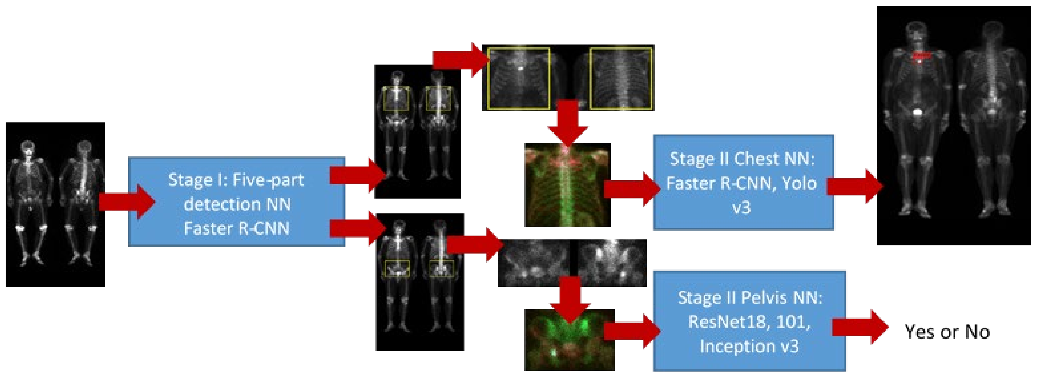
2.4. Detection of Five Body Parts
2.5. Pelvis NN
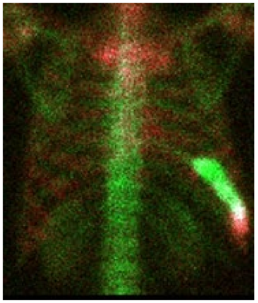
2.6. Chest NN
2.7. Training NN
2.7.1. Hard Negative Mining
2.7.2. Hard Positive Mining
2.8. Performance
3. Results
4. Discussion
5. Conclusions
Author Contributions
Funding
Institutional Review Board Statement
Acknowledgments
Conflicts of Interest
References
- National Health Insurance Research Database. Available online: https://www.mohw.gov.tw/cp-4256-48057-1.html (accessed on 10 April 2019).
- Bubendorf, L.; Schöpfer, A.; Wagner, U. Metastatic patterns of prostate cancer: An autopsy study of 1589 patients. Hum. Pathol. 2000, 31, 578–583. [Google Scholar] [CrossRef] [PubMed]
- Treating Prostate Cancer Spread to Bones. Available online: https://www.cancer.org/cancer/prostate-cancer/treating/treating-pain.html (accessed on 14 April 2020).
- Imbriaco, M. A new parameter for measuring metastatic bone involvement by prostate cancer: The Bone Scan Index. Clin. Cancer Res. 1998, 4, 1765–1772. [Google Scholar] [PubMed]
- Brown, M.S. Computer-Aided Bone Scan Assessment with Automated Lesion Detection and Quantitative Assessment of Bone Disease Burden Changes. U.S. Patent US20140105471, 7 April 2012. [Google Scholar]
- Ulmert, D. A Novel automated platform for quantifying the extent of skeletal tumour involvement in prostate cancer patients using the bone scan index. Eur. Urol. 2012, 62, 78–84. [Google Scholar] [CrossRef] [PubMed] [Green Version]
- Apiparakoon, T.; Rakratchatakul, N.; Chantadisai, M.; Vutrapongwatana, U. MaligNet: Semisupervised learning for bone lesion instance segmentation using bone scintigraphy. IEEE Access 2020, 8, 27047–27066. [Google Scholar] [CrossRef]
- Sun, P.; Wang, D.; Mok, V.-C.; Shi, L. Comparison of feature selection methods and machine learning classifiers for radiomics analysis in glioma grading. IEEE Access 2019, 7, 102010–102020. [Google Scholar] [CrossRef]
- Chen, Y.-H.; Lue, K.-H.; Chu, S.-C. Combing the radiomic features and traditional parameters of 18F-FDG PET with clinical profiles to improve prognostic stratification in patients with esophageal squamous cell carcinoma treated with neoadjuvant chemo-radiotherapy and surgery. Ann. Nucl. Med. 2019, 33, 657–670. [Google Scholar] [CrossRef] [PubMed]
- Alom, M.Z. A State-of-the-art Survey on Deep Learning Theory and Architectures. Electronics 2019, 8, 292. [Google Scholar] [CrossRef] [Green Version]
- Zhao, Z.Q. Object detection with deep learning: A review. IEEE Trans. Neural Netw. Learn. Syst. 2019, 30, 3212–3232. [Google Scholar] [CrossRef] [PubMed] [Green Version]
- Ren, S.; He, K.; Girshick, R.; Sun, J. Faster R-CNN: Towards real-time object detection with region proposal networks. IEEE Trans. Pattern Anal. Mach. Intell. 2017, 39, 1137–1149. [Google Scholar] [CrossRef] [PubMed] [Green Version]
- Redmon, J.; Divvala, S.; Girshick, R.; Farhadi, A. You Only Look Once: Unified, real-time object detection. In Proceedings of the IEEE Conference on Computer Vision and Pattern Recognition (CVPR 2016), Las Vegas, NV, USA, 27–30 June 2016. [Google Scholar]
- PyTorch-YOLOv3. Available online: https://github.com/eriklindernoren/PyTorch-YOLOv3 (accessed on 10 April 2021).
- Ioffe, S.; Szegedy, C. Batch normalization: Accelerating deep network training by reducing internal covariate shift. arXiv 2015, arXiv:1502.03167. [Google Scholar]
- Sung, K.; Poggio, T. Example-Based Learning for View Based Human Face Detection; Technical Report A.I. Memo No. 1521; Massachussets Institute of Technology: Cambridge, MA, USA, 1994. [Google Scholar]
- Felzenszwalb, P.; Girshick, R.; McAllester, D.; Ramanan, D. Object detection with discriminatively trained part based models. IEEE Trans. Pattern Anal. Mach. Intell. 2010, 32, 1627–1645. [Google Scholar] [CrossRef] [PubMed] [Green Version]
- Taiwan Computing Cloud. Available online: https://www.twcc.ai/ (accessed on 10 April 2021).
- Löfgren, J.; Mortensen, J.; Rasmussen, S.H.; Madsen, C.; Loft, A.; Hansen, A.E.; Oturai, P.; Jensen, K.E.; Mørk, M.L.; Reichkendler, M.; et al. A Prospective Study Com- paring 99mTc-Hydroxyethylene-Diphosphonate Planar Bone Scintigra- phy and Whole-Body SPECT/CT with 18F-Fluoride PET/CT and 18F-Flu- oride PET/MRI for Diagnosing Bone Metastases. J. Nucl. Med. 2017, 58, 1778–1785. [Google Scholar] [CrossRef] [PubMed] [Green Version]
- Pratt, L.Y.; Thrun, S. Machine Learning—Special Issue on Inductive Transfer; Springer: Berlin/Heidelberg, Germany, 1997. [Google Scholar]


| Shoulder | Rib | Spinal Cord | Pelvis | Thigh | |
|---|---|---|---|---|---|
| Confirmed metastasis | 315 | 602 | 399 | 311 | 198 |
| Normal lesion | 31 | 81 | 39 | 25 | 11 |
| Inception v3 | ResNet 18 | ResNet 101 | |
|---|---|---|---|
| Sensitivity | 0.84 ± 0.13 | 0.80 ± 0.15 | 0.87 ± 0.12 |
| Specificity | 0.81 ± 0.12 | 0.81 ± 0.12 | 0.81 ± 0.11 |
| Yolo v3 | Faster R CNN | |
|---|---|---|
| Sensitivity | 0.82 ± 0.08 | 0.70 ± 0.04 |
| Precision | 0.70 ± 0.11 | 0.69 ± 0.07 |
| Model | Learning Rate | Batch Size | Epoch |
|---|---|---|---|
| Faster R CNN | 0.0001 | 16 | 40 |
| Yolo v3 | 0.000579 | 32 | 100 |
| ResNet 18 | 0.001 | 8 | 50 |
| ResNet 101 | 0.001 | 8 | 50 |
| Inception v3 | 0.001 | 8 | 50 |
Publisher’s Note: MDPI stays neutral with regard to jurisdictional claims in published maps and institutional affiliations. |
© 2021 by the authors. Licensee MDPI, Basel, Switzerland. This article is an open access article distributed under the terms and conditions of the Creative Commons Attribution (CC BY) license (https://creativecommons.org/licenses/by/4.0/).
Share and Cite
Cheng, D.-C.; Liu, C.-C.; Hsieh, T.-C.; Yen, K.-Y.; Kao, C.-H. Bone Metastasis Detection in the Chest and Pelvis from a Whole-Body Bone Scan Using Deep Learning and a Small Dataset. Electronics 2021, 10, 1201. https://doi.org/10.3390/electronics10101201
Cheng D-C, Liu C-C, Hsieh T-C, Yen K-Y, Kao C-H. Bone Metastasis Detection in the Chest and Pelvis from a Whole-Body Bone Scan Using Deep Learning and a Small Dataset. Electronics. 2021; 10(10):1201. https://doi.org/10.3390/electronics10101201
Chicago/Turabian StyleCheng, Da-Chuan, Chia-Chuan Liu, Te-Chun Hsieh, Kuo-Yang Yen, and Chia-Hung Kao. 2021. "Bone Metastasis Detection in the Chest and Pelvis from a Whole-Body Bone Scan Using Deep Learning and a Small Dataset" Electronics 10, no. 10: 1201. https://doi.org/10.3390/electronics10101201
APA StyleCheng, D.-C., Liu, C.-C., Hsieh, T.-C., Yen, K.-Y., & Kao, C.-H. (2021). Bone Metastasis Detection in the Chest and Pelvis from a Whole-Body Bone Scan Using Deep Learning and a Small Dataset. Electronics, 10(10), 1201. https://doi.org/10.3390/electronics10101201