Article

The Impacts of Atmospheric Stability on the Accuracy of Wind Speed Extrapolation Methods

School of Meteorology, University of Oklahoma, 120 David L. Boren Blvd., Norman, OK 73072, USA
*
Author to whom correspondence should be addressed.
Resources 2014, 3(1), 81-105; https://doi.org/10.3390/resources3010081
Submission received: 3 December 2013 / Revised: 25 December 2013 / Accepted: 8 January 2014 / Published: 23 January 2014
(This article belongs to the Special Issue Spatial and Temporal Variation of the Wind Resource)

Abstract

:
The building of utility-scale wind farms requires knowledge of the wind speed climatology at hub height (typically 80–100 m). As most wind speed measurements are taken at 10 m above ground level, efforts are being made to relate 10-m measurements to approximate hub-height wind speeds. One common extrapolation method is the power law, which uses a shear parameter to estimate the wind shear between a reference height and hub height. The shear parameter is dependent on atmospheric stability and should ideally be determined independently for different atmospheric stability regimes. In this paper, data from the Oklahoma Mesonet are used to classify atmospheric stability and to develop stability-dependent power law fits for a nearby tall tower. Shear exponents developed from one month of data are applied to data from different seasons to determine the robustness of the power law method. In addition, similarity theory-based methods are investigated as possible alternatives to the power law. Results indicate that the power law method performs better than similarity theory methods, particularly under stable conditions, and can easily be applied to wind speed data from different seasons. In addition, the importance of using co-located near-surface and hub-height wind speed measurements to develop extrapolation fits is highlighted.

1. Introduction

Environmental concerns and rising fossil fuel prices have prompted rapid development in the renewable energy sector. Wind energy, in particular, is projected to emerge as one of the fastest-growing renewable energy technologies in the world [1]. In fact, the United States Department of Energy has examined a scenario in which 20% of the energy needs of the United States are provided by wind energy by the year 2030 [2]. Such a scenario could reduce annual carbon dioxide emissions from the energy sector by 825 million metric tons, but would require a large increase in the installed wind capacity in the United States [2].
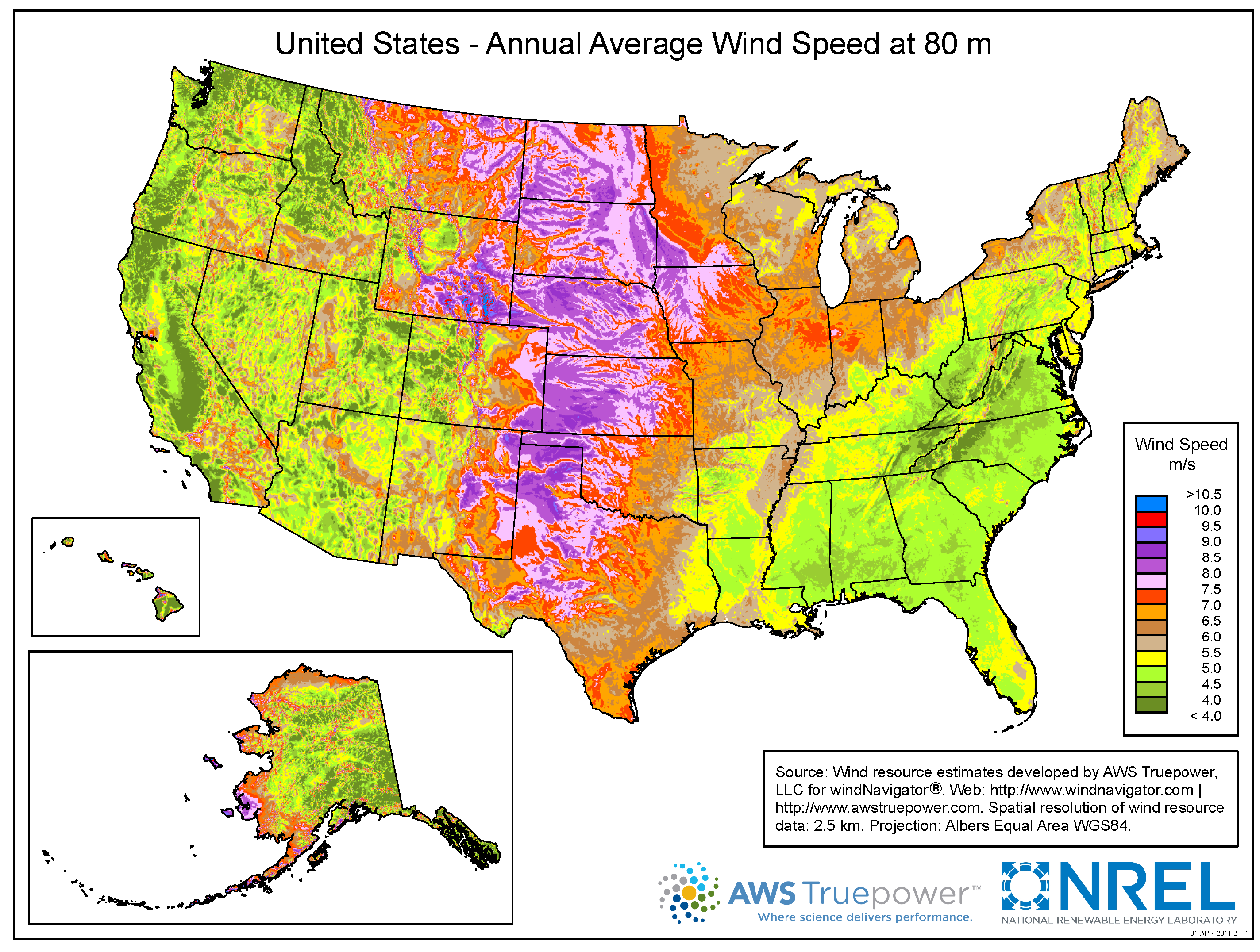
It has been estimated that the Great Plains region of the United States possesses the country’s highest wind power potential (Figure 1). The land in the Great Plains is mostly flat and located far away from both ocean coasts. This lack of complex terrain allows wind to flow unimpeded for great distances, which, in addition to the prominence of the nocturnal low-level jet, creates a vast, largely untapped potential for wind power in the Great Plains. However, wind farm siting is often a meticulous process that requires examining the site’s wind climatology at turbine hub heights, which typically range from 60 to 100 m above ground level (a.g.l.) [3]. As most standard meteorological observation sites were not designed for wind energy applications, there is a substantial lack of meteorological data at these heights [4]. Tall meteorological towers are expensive to operate and maintain, and many tall towers that have been deployed at future wind farm sites do not reach the projected turbine hub height [5]. Thus, researchers and wind energy developers are often forced to extrapolate wind speed data from available observation stations to typical hub heights to estimate the expected hub-height wind speed climatology (e.g., [3]).
Figure 1. Wind resource map for the United States. The Great Plains region is the large, north-south oriented area in the center of the country that is largely shaded in red and purple. From U.S. Department of Energy [6].
Resources 03 00081 g001
The most widely used extrapolation method is the power law, a method that relies only on the wind speed at a reference height (typically 10 m a.g.l.) and a shear exponent, p, that governs the amount of wind shear between the reference height and the turbine hub height [7]. Traditionally, the shear exponent has been set to a value of 1/7, which is assumed to be associated with neutral atmospheric conditions. However, the actual value of the shear exponent varies with atmospheric stability and surface roughness (e.g., [7,8,9,10,11]). Thus, stability information is needed to separate wind speed data into atmospheric stability classes if one wishes to develop power law fits for different atmospheric stability conditions.
Two commonly used stability parameters are the Obukhov length and the gradient Richardson number. The Obukhov length calculation requires measurements of heat and momentum fluxes (typically from a sonic anemometer), while the Richardson number calculation requires temperature measurements at two different levels to estimate the vertical temperature gradient [12]. Unfortunately, cup anemometers are widely used instead of sonic anemometers on surface stations due to the large difference in instrument cost, and cup anemometers do not have adequate accuracy or temporal resolution to measure fluxes [13]. World Meteorological Organization Guidelines only recommend measuring air temperature at a height of 2 m a.g.l. [14], which precludes the estimation of the gradient Richardson number at nearly all surface observation stations.
However, the Oklahoma Mesonet, a statewide network of surface observation stations, provides wind speed and temperature measurements at two levels to facilitate the estimation of vertical temperature and wind speed gradients. In addition, several tall meteorological towers are in operation across Oklahoma, with some towers located in close proximity to the Mesonet sites. Thus, Mesonet data could potentially be used to characterize atmospheric stability near future wind farm sites and to develop stability-dependent power law fits. The availability of low-level stability information and hub-height wind speed measurements in Oklahoma provides a unique opportunity to study the effects of stability on extrapolation methods.
This work explores the use of Mesonet data to classify wind speeds by a stability regime and to improve upon the standard p = 1 / 7 power law fit by incorporating stability information. Power law fits are developed for different atmospheric stability regimes using low-level Mesonet temperature and wind speed data and 80-m wind speed data from a nearby tall tower. Power law fits developed from one month of data are then applied to data from different seasons to investigate the robustness of the power law method. Similarity theory is also explored as a possible alternative to the traditional power law method. Additionally, the impact of extrapolating 10-m wind speeds from a sensor that is not co-located with the 80-m wind sensor is investigated.
This paper provides new insights about the accuracy of various extrapolation methods for different stability regimes. The spatial variability of extrapolation parameters is also studied. Such information is critical for hub-height wind speed climatologies that are based on near-surface wind observations and could provide valuable new findings for wind energy developers, who must often use extrapolation methods when hub-height wind speed data are not available.

2. Background

2.1. Data Sources

The Oklahoma Mesonet is comprised of over 110 surface observation stations across the state of Oklahoma. Jointly operated by the University of Oklahoma and Oklahoma State University, the Mesonet began network-wide data collection in 1994. Every five minutes, each Mesonet site reports standard surface variables, including solar radiation, rainfall, pressure, air temperature and wind speed. Air temperature is measured with thermistors at 1.5 and 9 m a.g.l. Cup anemometers provide wind speed at 2 m, and wind monitors provide wind speed and direction at 10 m [15].
Tall data collection towers in Oklahoma are maintained by the Oklahoma Wind Power Initiative (OWPI), housed at the University of Oklahoma. Several towers were constructed near potential wind farm sites, and in some locations, wind instrumentation was added to existing communication towers. Wind speed and direction are measured by cup anemometers and wind vanes at several heights, ranging from 10 m to 80 or 100 m at some of the higher towers. At some heights, anemometers are located on two opposite sides of the mast, so that at least one of the anemometers will be relatively unaffected by mast shadowing at all times. More information can be found on the OWPI website [16].
The use of meteorological towers is not always ideal for wind energy studies. As wind power production is affected by wind speeds throughout the swept rotor disk area (e.g., [17]), it is important to measure wind speeds at several heights within the rotor disk. Due to limitations in tower height, these wind speed measurements could be made most easily by a remote sensing device (e.g., LiDAR; [18]). However, wind energy developers have historically used cup anemometers on meteorological towers to estimate the wind resource at potential wind farm sites. Although remote sensing devices are gaining popularity as useful tools in wind resource assessment studies, meteorological towers are still commonly used by wind energy developers [5]. Furthermore, in many instances, tower data are only available up to 50 or 60 m a.g.l., and wind energy developers are forced to use extrapolation methods to estimate the mean hub-height wind speed [5]. Thus, we felt that an extrapolation study with meteorological towers would still produce valuable results for the wind energy community, despite the shortcomings of meteorological towers.

2.2. Extrapolation Methods

In this work, several different approaches are used to produce correlations between 10- and 80-m wind speeds. The first approach involves the use of a traditional power law to relate wind speeds at different heights to a reference wind speed at a reference height close to the ground (typically, 10 m a.g.l.). The power law that is commonly used in the wind energy field is defined by the following equation:
u ( z ) = u r e f z z r e f p
where u ( z ) is the wind speed at height z, u r e f is the wind speed at height z r e f and p is the power law or shear exponent. Traditionally, neutral atmospheric conditions have been associated with p = 1 / 7 , with values higher (lower) than 1/7 indicating stable (unstable) conditions [7]. High values of the shear exponent indicate that the wind speed changes rapidly with height, which is common in stable regimes when the surface layer is decoupled from the rest of the boundary layer and vertical momentum transport is limited. In contrast, low values of the shear exponent indicate that wind speeds are fairly uniform with height, which is common during unstable regimes with substantial vertical mixing [19]. In locations with a large degree of surface heating, the shear exponent changes drastically throughout the day in response to the diurnal cycle of stability and vertical wind shear (e.g., [11]).
In the traditional power law, the shear exponent is determined solely from 10- and 80-m wind speed data and does not directly incorporate stability information. However, a stability parameter, such as the gradient Richardson number, can be used to classify wind speed data pairs by stability regime so that separate power law fits can be developed for each stability classification. A direct dependence of the shear exponent, p, on the Richardson number, R i , can be deduced through the use of similarity theory. Monin–Obukhov Similarity Theory (MOST) employs a modified “log-law” equation to estimate the mean wind speed at different heights, z, a.g.l.:
u ¯ ( z ) = u * κ l n z z o - Ψ m ( ζ )
u * is the friction velocity, z o is the roughness length and Ψ m ( ζ ) is a stability correction factor. ζ is the height above ground, z, normalized by the Obukhov length, L, where L = - u * 3 θ v ¯ κ g w θ v ¯ . θ v ¯ is the mean virtual potential temperature at the measurement height, κ is the von Kármán constant (commonly set to 0.4), g is the acceleration due to gravity and w θ v ¯ is the heat flux measured at the surface [12].
The MOST fit (Equation (2)) produces a logarithmic wind speed profile. By combining the power law equation with MOST, a power law fit can be developed that relates the shear exponent, p, to the gradient Richardson number. This method is described in Section 4.2.
One advantage of similarity theory-based methods is that they do not require 80-m wind speed data to develop the extrapolation fits; 80-m data are only needed to evaluate the accuracy of the extrapolations. In contrast, the power law method requires wind speeds at 10 and 80 m. This is problematic if only near-surface information is available, e.g., from a Mesonet-type station. Small, 10-m towers are much easier and less costly to build and maintain in comparison to 80-m tall towers (e.g., [18]); in addition, tall towers do not usually include temperature information, which is needed to calculate standard stability parameters. In the state of Oklahoma, which has high wind resource potential (Figure 1), there are over 100 10-m Mesonet sites that have been operated nearly continuously since 1994 [15], while only a handful of tall towers have been in operation sporadically in the past decade. Thus, it is advantageous to use a method that requires only low-level data to develop an extrapolation fit.
However, similarity theory also has some disadvantages. A major disadvantage of MOST is that it assumes fluxes are constant with height, which is typically only valid in the surface layer. Thus, the accuracy of MOST tends to decrease with increasing height, particularly for stable atmospheric conditions, where the surface layer can be very shallow [20,21]. In order to overcome this limitation, Gryning et al. [21] developed a new set of relations to extend the wind profile above the surface layer. This method, hereafter referred to as Extended MOST (EMOST), uses a set of length scales to estimate the wind speed profile. The characteristic wind profile length scale, l, is related to unique length scales in the surface layer, middle boundary layer and upper boundary layer through inverse summation:
1 l = 1 L S L + 1 L M B L + 1 L U B L
In the method of Gryning et al. [21], the following general equation is used to estimate the wind speed profile for different stability conditions:
u ¯ ( z ) = u * κ l n z z o - Ψ m ( ζ ) S t a b i l i t y + z L M B L M i d d l e B L - z z i z 2 L M B L U p p e r B L
Ψ m ( ζ ) is a stability correction factor, similar to the stability parameter in MOST; L M B L is the length scale in the middle boundary layer and z i is the boundary layer height.

3. Wind Speed Data

Wind speed data from the month of August 2009 were used as a training dataset for this study. The month of August was chosen because the weather is typically quiescent in Oklahoma throughout the late summer. An analysis of 500-mb height charts during this period indicates that flow was zonal for most of the data collection period, with a large ridge over much of the Southern Plains. Thus, variations in wind speed were likely influenced primarily by diurnal variations. After initial analysis of the August, 2009 data, the extrapolation methods were then applied to data throughout the remainder of 2009 to examine seasonal influences on the extrapolation methods.
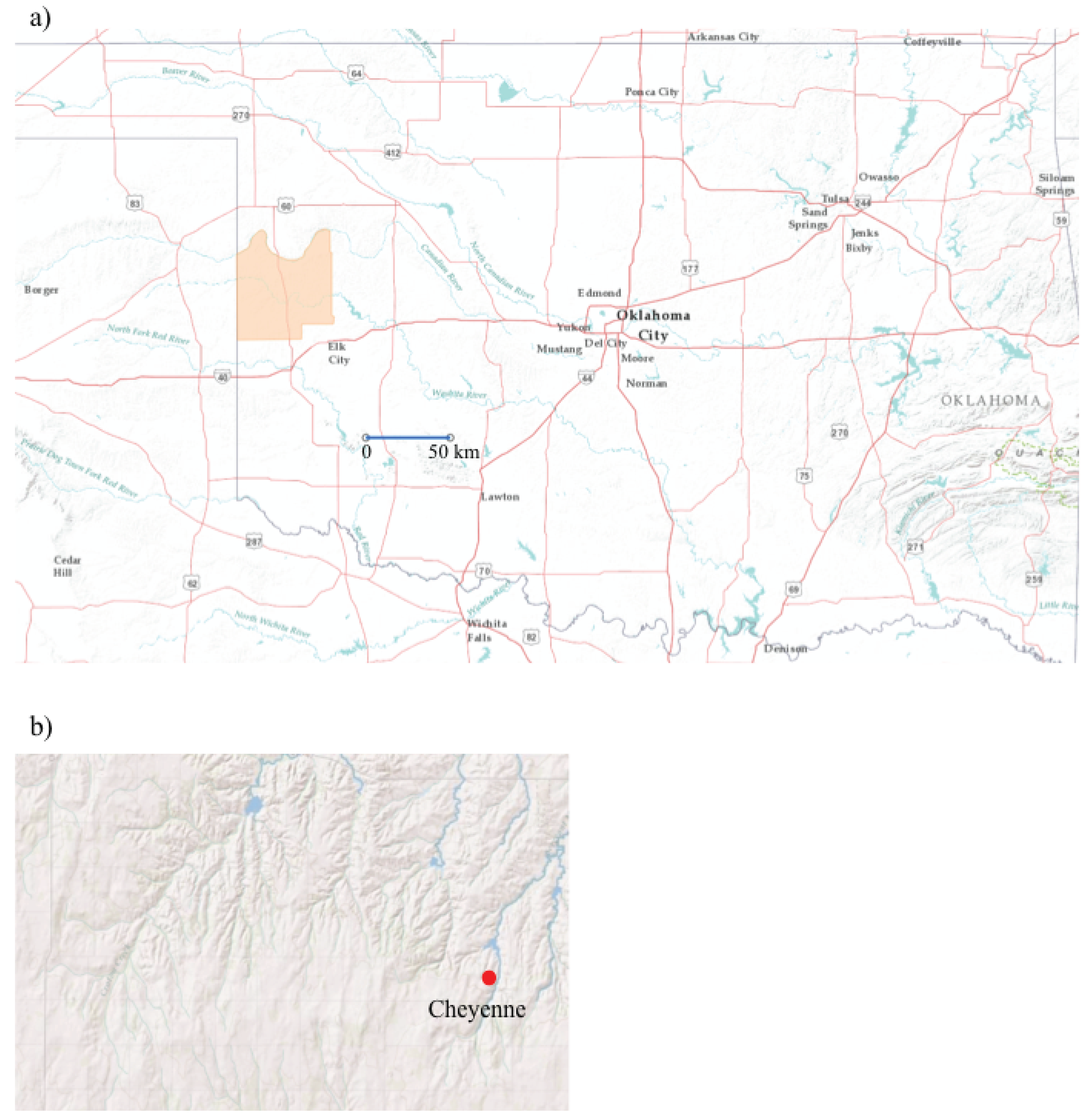
Wind speed data at 80 m were obtained from a tall tower in Roger Mills County. Because the data are proprietary, the exact location of the tall tower cannot be disclosed; however, the tall tower was located within 25 km of the Cheyenne Mesonet site (Figure 2a,b). The Cheyenne Mesonet site was used to obtain 2- and 10-m wind speed data, as well as 1.5-m and 9-m temperature data. Wind speed data from the tall tower are available in 10-min averages, while Mesonet data are available in 5-min averages. The Mesonet data were thus further averaged to match the tall tower 10-min data. Data pairs where the Mesonet wind speed at 10 m exceeded the tower wind speed at 80 m were removed, as the extrapolation methods tested assume that wind speed increases with height. This resulted in the removal of approximately 3% of the wind speed data pairs in August, 2009. Cup anemometers were located on the north and south sides of the tall tower at 80 m, so wind direction information was used to select wind speed data that were not directly affected by the mast.
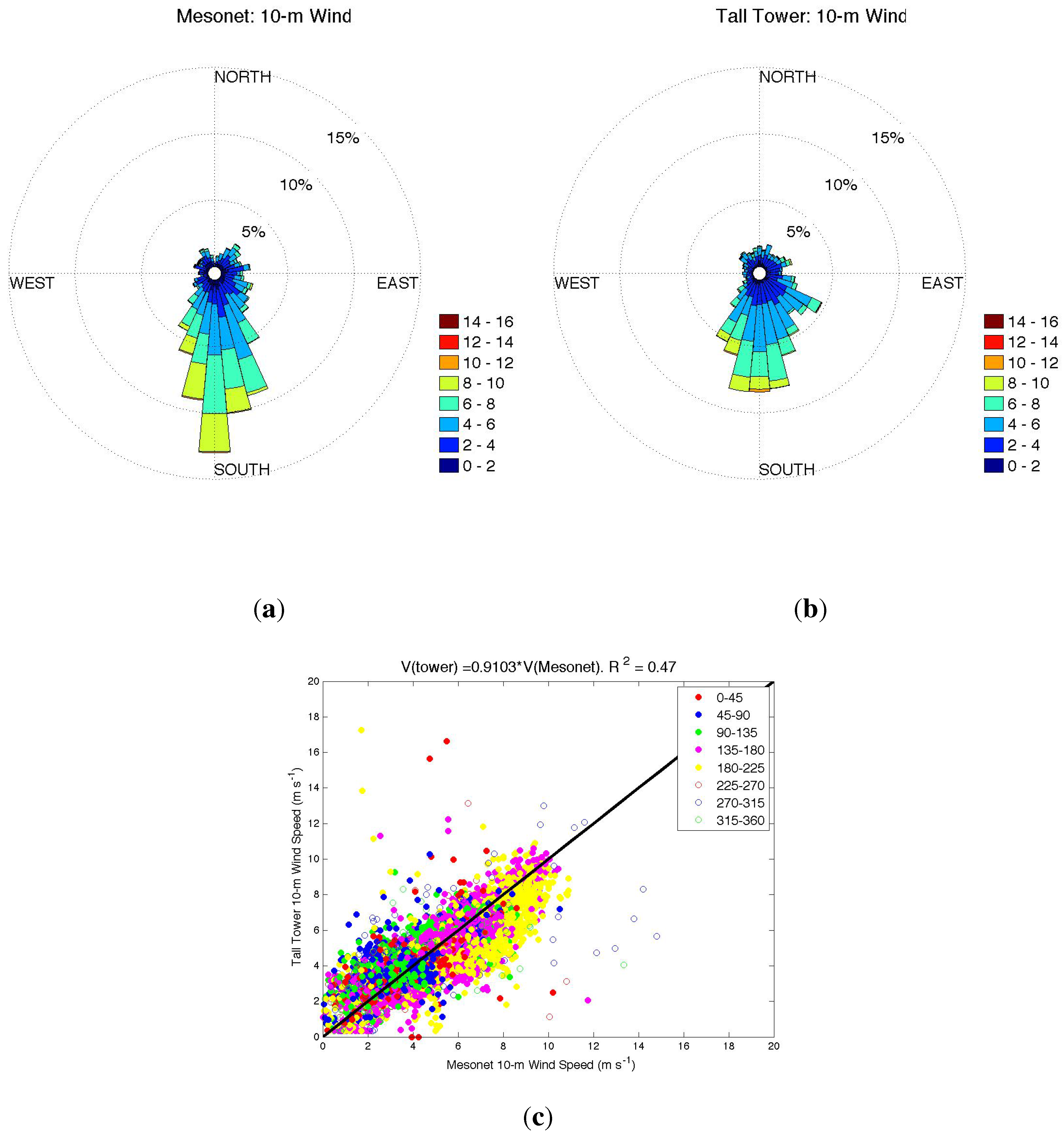
Throughout 2009, tall tower data were available at 10, 50 and 80 m. As the Mesonet site and tall tower were located in a region with moderate topography (Figure 2b), it is likely that the Mesonet and tall tower experienced different wind speed and direction distributions. As shown in Figure 3a,b, for the 10-m measurement height, winds were primarily from the south at the Mesonet site during August 2009, while the winds experienced at the tall tower site more frequently had south-easterly and south-westerly components.
While the wind speeds at the sites were generally in agreement (Figure 3c), large deviations sometimes occurred. In particular, the Mesonet site tended to measure higher wind speeds than the tall tower site when the wind was south-easterly to south-westerly (135 –225 ), while the reverse was true when winds had a stronger easterly component (45 –135 ) (Figure 3c). The Mesonet site is located on the southern end of a north-south oriented ridge (Figure 2b), so it is possible that winds from the south accelerated as they moved up the ridge to the Mesonet site. In addition, winds coming from the south toward the tall tower may have been blocked by a nearby obstruction [22]. It is unclear why differences occur between the two sites for winds with an easterly component.
Figure 2. (a) Map of the state of Oklahoma displayed using ArcGIS software package. Roger Mills county is shaded in orange; (b) Zoomed-in map of Roger Mills county in western Oklahoma. The Cheyenne Mesonet site is indicated by a red marker. The tall tower used in the study is located in the western part of the county.
Resources 03 00081 g002
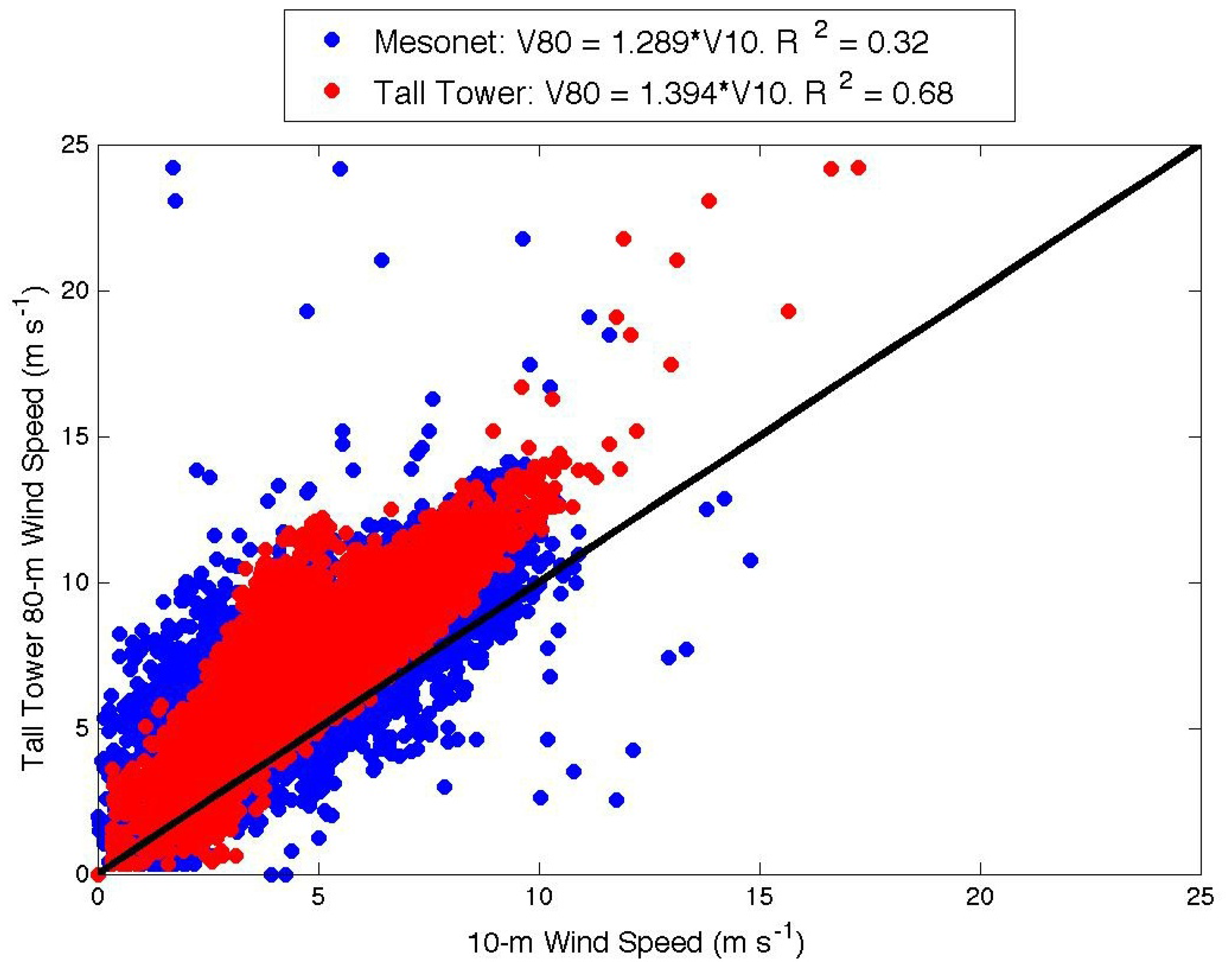
The majority of 10-m wind speeds measured at both the Mesonet site and the tall tower site were lower than the 80-m wind speeds measured by the tall tower (Figure 4). However, the 10-m wind speeds measured by the tall tower had a much stronger correlation to the 80-m tall tower wind speeds ( R 2 = 0.68) in comparison to the 10-m Mesonet wind speeds ( R 2 = 0.32; Figure 4). In Section 4, both the Mesonet and tall tower 10-m wind speeds are used in the various extrapolation methods to examine the effect of the spatial separation of the sites on the accuracy of the extrapolations. This information is needed to assess whether the wind climatologies from observational networks, such as the Oklahoma Mesonet, can be applied over a large region or if local effects cause strong deviations.
Figure 3. (a) Ten-meter wind rose for August 2009, at Cheyenne Mesonet site; (b) 10-m wind rose for August 2009, at the tall tower; and (c) scatter plot of 10-m Mesonet wind speeds and 10-m tall tower wind speeds during August 2009. In (c), colors correspond to wind directions measured in degrees at the Mesonet site, and the solid black line shows the 1:1 line. Wind speeds are given in m s - 1 .
Resources 03 00081 g003
Further information can be gleaned by separating the wind speed data pairs by the atmospheric stability regime. Since wind speed and temperature data were available at two levels at the Mesonet site, the gradient Richardson number, R i , was calculated for use as a stability parameter:
R i = g T o θ z ( u z ) 2
where g is the gravitational acceleration; T o is the surface temperature and u z and θ z are the vertical gradients of wind speed and potential temperature, respectively. In this study, R i was calculated from the Cheyenne Mesonet station following the finite-differencing method of Bodine et al. [23]:
R i = g [ ( T 9 m - T 1 . 5 m ) / Δ z T + Γ d ) ] Δ z u 2 T 1 . 5 m ( u 10 m - u 2 m ) 2
where T 9 m and T 1 . 5 m are the temperatures at 9 and 1.5 m a.g.l., respectively; u 10 m and u 2 m are the wind speed magnitudes at 10 and 2 m a.g.l., respectively; and Δ z T and Δ z u refer to the differences in measurement levels for T and u. The vertical gradient of potential temperature is approximated by adding the dry adiabatic lapse rate, Γ d , to the vertical temperature gradient. Ten-minute averages of the wind speed and temperature data were used to update R i every 10 min.
Figure 4. Scatter plot of 10-m wind speeds measured at the Mesonet site (blue) and the tall tower (red) compared to 80-m wind speeds measured at the tall tower during August 2009. The solid black line shows the 1:1 line.
Resources 03 00081 g004
In this work, stability classifications were loosely based on the classifications of Mauritsen and Svensson [24] and defined as follows:
  • Strongly unstable: R i < - 0 . 2 ;
  • Unstable: - 0 . 2 R i < - 0 . 1 ;
  • Neutral: - 0 . 1 R i < 0 . 1 ;
  • Stable: 0 . 1 R i < 0 . 25 ;
  • Strongly stable: R i 0 . 25 ;
According to these classifications, nearly 50% of the wind speed data pairs in August 2009, occurred during a neutral regime, while approximately 20% occurred during an unstable regime and 30% during a stable regime. Unfortunately, temperature measurements were only made at the Mesonet sites, so it was assumed that stability conditions experienced at the tall tower site were similar to those experienced at the Mesonet site. As most wind farms do not have on-site temperature profile measurements, it is not uncommon to use information from an off-site sensor to determine stability (e.g., [25]).
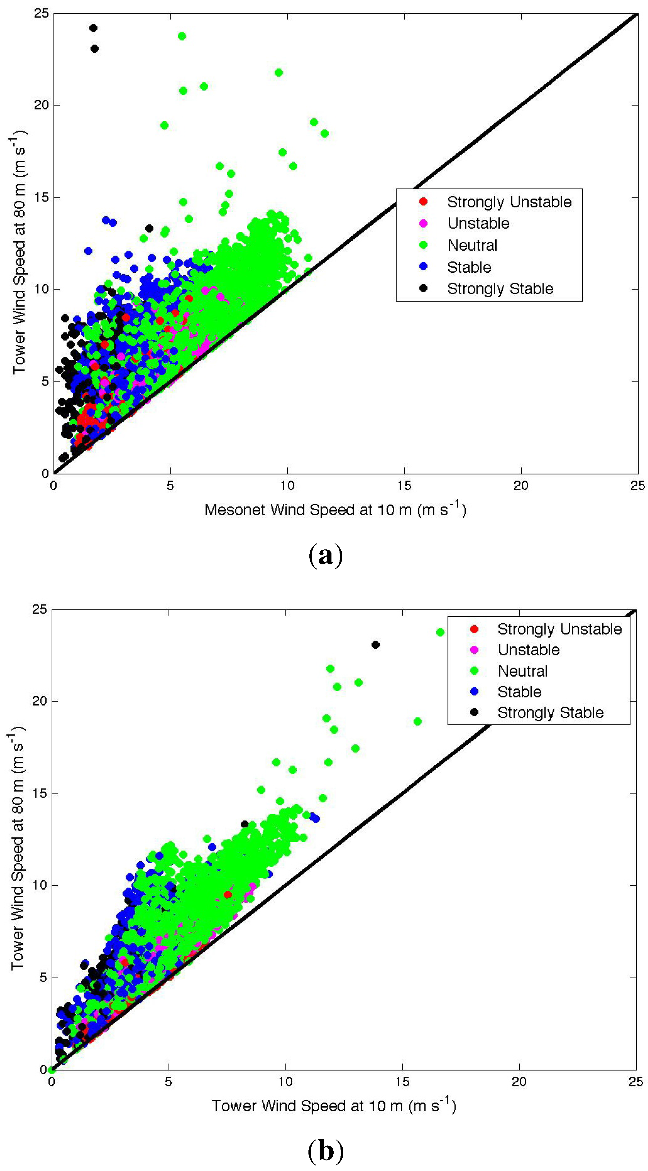
Figure 5. Ten-meter wind speeds vs. 80-m wind speeds as a function of atmospheric stability during August 2009. (a) Ten-meter Mesonet wind speed vs. 80-m tall tower wind speed; and (b) 10-m tall tower wind speed vs. 80-m tall tower wind speed. Data pairs where the 10-m wind speed exceeded the 80-m wind speed were removed to avoid violating the assumptions of the extrapolation methods.
Resources 03 00081 g005
Scatter plots of 10- and 80-m winds stratified by stability classification for August 2009, are shown in Figure 5. As first shown in Figure 4, the 10-m tall tower wind speeds are much more correlated to the 80-m tall tower wind speeds in comparison to the 10-m Mesonet wind speeds. However, Figure 5 a,b shows an approximately one-to-one correlation between 10- and 80-m wind speeds under unstable conditions for both the Mesonet and tall tower data. This correlation is expected, since well-mixed, uniform profiles of wind speed are typically observed under unstable conditions, for which spatial variability is also less pronounced in comparison to stable conditions [19]. The correlations between the 10- and 80-m wind speeds begin to deviate for neutral and stable conditions. Most of the observations corresponding to neutral and stable conditions are located well above the one-to-one line, indicating that 80-m wind speeds are much higher than 10-m wind speeds and that wind shear exists in the vertical direction (Figure 5). However, the wind shear between the 10-m Mesonet measurements and the 80-m tall tower measurements (Figure 5 a) is much higher than the shear between the tall tower measurements at 10 and 80 m for neutral and stable conditions (Figure 5 b).

4. Extrapolation Methods: Results

In this section, the 10- and 80-m wind speed data for the month of August, 2009, are fit to a power law. The power law and similarity theory methods are then combined to produce a Mesonet-derived power law fit. The accuracy of these extrapolation methods is explored for different stability regimes and different seasons. In addition, Monin–Obukhov similarity theory and the extended Monin–Obukhov similarity theory of Gryning et al. [21] are investigated as possible alternatives to the power law method.

4.1. Power Law

First, the wind speed data were used to fit a power law of the form u ( z ) = u r e f ( z z r e f ) p . u r e f was taken to be the wind speed measured at 10 m at the Cheyenne Mesonet site and the tall tower, as 10 m is a common reference level used to fit the power law in wind energy studies [7]. The statistics toolbox in MATLAB was used to fit a linear regression to the wind speed data, and a best-fit line of the form u ( 80 m ) = u ( 10 m ) × s l o p e was found. For a power law fit, the slope is equal to ( z / z r e f ) p . Solving for p gives p = l n ( s l o p e ) / l n ( z / z r e f ) = l n ( s l o p e ) / l n ( 80 / 10 ) . For each stability class, a different value of p was determined, which was then used to calculate 80-m wind speeds from 10-m wind speeds.
Values of the shear exponent, p, the coefficient of determination, R 2 , and the root-mean-squared error (RMSE) for the traditional power law fit are shown in Table 1. Values of R 2 and RMSE for a power law fit with a constant shear exponent of 1/7 (≈ 0 . 143 ) are shown for comparison. For the traditional power law fit, the value of p approximated from the wind speed data generally increased with increasing stability (Table 1), indicating that the amount of vertical wind shear increased with increasing stability, as expected [7]. The neutral values of the shear exponent were quite close to the assumed neutral value of 1/7. The use of 10-m tall tower data in the power law fit produced slightly lower shear exponent values for most of the stability classes (Table 1). This suggests that using the Mesonet 10-m wind speed data leads to an overestimation of vertical wind shear between 10 and 80 m.
For the month of August, 2009, the power law produced higher R 2 values for unstable regimes and lower R 2 values for stable regimes. Not surprisingly, the power law fit was much more accurate when tall tower data were used for the 10-m wind speed values. In particular, the R 2 value for the strongly stable regime increased from 0.78 to 0.96 when the tall tower data were used for the 10-m reference wind speeds (Table 1). This lower R 2 value for the Mesonet 10-m data was likely related to the overestimation of vertical wind shear when 10-m Mesonet data were used.
Table 1. The coefficient of determination ( R 2 ) and root-mean-squared error (RMSE) values for different power law fits for all stability classes. Shear exponent values for the traditional power law fit are also shown. Ten-meter wind speed data from the Mesonet and tall tower were evaluated separately to produce power law fits.
Traditional Power Law: Shear Exponent
Month, 10-m Data SourceStrongly UnstableUnstableNeutralStableStrongly Stable
August 2009, Mesonet0.120.090.130.280.39
August 2009, Tall Tower0.060.080.160.260.28
p = 1/7: R 2
August 2009, Mesonet0.970.970.960.860.66
August 2009, Tall Tower0.960.970.970.910.90
Traditional Power Law: R 2
August 2009, Mesonet0.970.980.960.920.78
August 2009, Tall Tower1.00.990.970.960.96
Mesonet-Derived Power Law: R 2
August 2009, Mesonet0.970.980.960.930.86
August 2009, Tall Tower0.990.990.960.920.94
p = 1/7: RMSE (m s - 1 )
August 2009, Mesonet0.941.11.82.73.5
August 2009, Tall Tower1.00.961.42.11.8
Traditional Power Law: RMSE (m s - 1 )
August 2009, Mesonet0.880.851.82.12.8
August 2009, Tall Tower0.330.491.41.51.2
Mesonet-Derived Power Law: RMSE (m s - 1 )
August 2009, Mesonet0.940.851.71.92.1
August 2009, Tall Tower0.390.621.82.01.4
The use of stability information to determine different shear exponents for different stability classes did not have a large effect on the R 2 values for unstable regimes, but served to increase the R 2 values significantly for stable regimes. In addition, RMSE values for all stability regimes (with the exception of the neutral regime) for both the Mesonet and the tall tower fit decreased when stability information was used to determine shear exponent values. The increase in R 2 values for stable regimes is likely related to the large deviation of the shear exponent from the neutral 1/7 value, as the atmosphere becomes more stable (Table 1). Co-located 10- and 80-m wind speed data from Cabauw, The Netherlands, also indicate that the shear exponent tends to be close to the neutral value under daytime, unstable conditions, but increases substantially above the neutral value under nighttime, stable conditions [11].

4.2. Mesonet-Derived Power Law

Next, the power law and similarity theory methods were combined to develop power law fits from the Mesonet data in a technique similar to that used by Panofsky et al. [26]. This method involves manipulating equations for the power law fit and similarity theory to find the shear parameter, p, as a function of atmospheric stability.
First, differentiating Equation (1) with respect to z gives:
u z = p u r e f z z r e f p 1 z = p u ( z ) z
Another expression for u z can be obtained through the use of similarity theory, by utilizing the MOST equation for the vertical wind speed gradient:
u z = u * κ z ϕ m z L
where ϕ m z L is the similarity function for momentum. Equating the right-hand sides of Equations (7) and (8) and solving for p gives the following equation:
p = u * u ( z ) z κ z ϕ m z L = C D κ ϕ m z L
where the ratio, u * u ( z ) , is defined as the square root of the drag coefficient, C D [12]. Equation (9) can be further simplified by defining a value of the shear parameter under neutral conditions, p o . If we let p o = C D κ , then Equation (9) becomes the following:
p = p o ϕ m z L
If we assume that the effects of surface roughness and stability on the shear parameter can be separated, then all roughness effects are described by the value of p o and all stability effects are incorporated into ϕ m z L . For this study, p o was simply defined as the shear parameter fit for neutral conditions (Table 1), with different values for the Mesonet fit and the tall tower fit. However, the value of the shear exponent does vary with surface roughness and has a stronger variation for unstable conditions [9]. In the future, different variables, such as wind direction, could be used to determine values for p o that depend more strongly on the upwind fetch, and thus, the roughness length, which impacts the wind speeds at the measurement site.
The similarity function for momentum, ϕ m z m L , is typically related to R i through the use of the following empirical relations:
ζ m = z m L = R i ; R i < 0
ζ m = z m L = R i 1 - 5 R i ; 0 R i < 0 . 2
ϕ m z m L = 1 + 5 ζ m ; ζ m 0
ϕ m z m L = ( 1 - 15 ζ m ) - 1 / 4 ; ζ m < 0
where z m is the mean geometric height used for the calculation of R i . For the Mesonet-derived power law fit, these similarity relations were used as a basis to develop a parameterization for p as a function of R i . Note that in Equations (13) and (14), ϕ m is given as a function of z m L , while ϕ m is given as a function of z L in Equation (10). However, z m L and z L are related through the simple equation z L = z m L z z m , where the ratio, z z m , is constant for a given value of z.
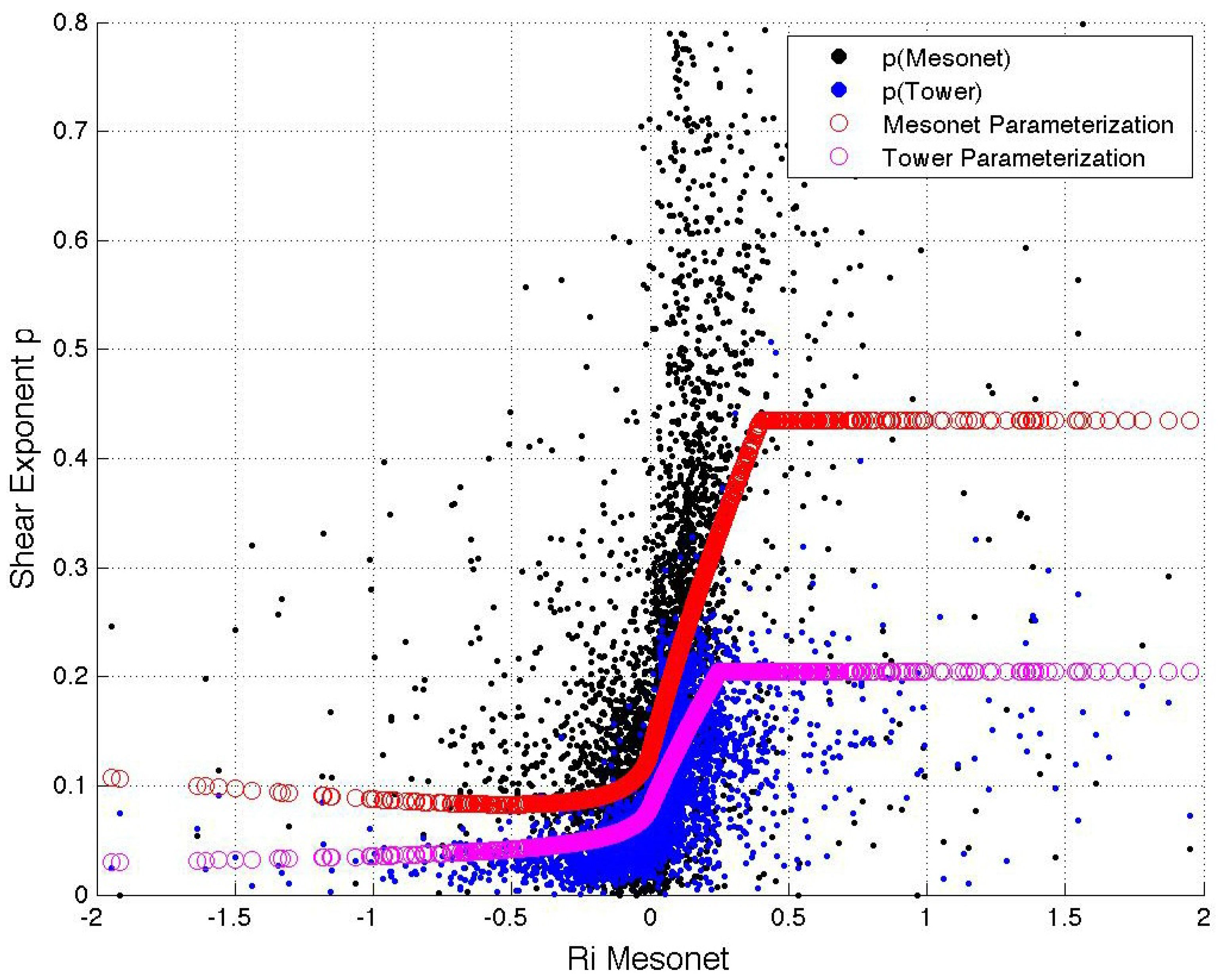
Scatter plots of Richardson number and shear parameters determined from the Mesonet and tall tower 10-m data are shown in Figure 6. Although the relationship between p and R i largely followed the similarity functions outlined in Equations (11)–(14), some fine-tuning was needed to produce a more accurate fit. For both stable and unstable conditions, equations of the following form were developed:
p = p o ( 1 + a R i ) b
where values of a and b were determined separately for stable and unstable regimes and different values of p o were defined for the Mesonet and tower fits.
Figure 6. Scatter plot of the gradient Richardson number measured at the Cheyenne Mesonet site and shear parameter values determined from 10-m Mesonet and tall tower data and 80-m tall tower data for August, 2009. Parameterizations for p as a function of R i are shown with dotted red and magenta lines.
Resources 03 00081 g006
The Mesonet neutral shear exponent, 0.13, was used for p o for the Mesonet parameterizations, while the tower unstable shear exponent, 0.08, was used for the tower parameterizations. The unstable tower shear exponent was used instead of the neutral shear exponent, because it provided a much better fit to the data in Figure 6. As shown in Table 1, the tower shear exponent for neutral conditions was 0.16, twice the value of the shear exponent for unstable conditions. Using the value of 0.16 would increase the parameterized p values in Figure 6 and provide a much poorer fit to the actual shear exponent values. It is likely that more accurate values of p o could be determined if stability information was available at the tall tower site.
For the parameterization under stable conditions ( R i > 0 ), our empirical fit provided a = 10 and b = 0 . 75 . A critical Richardson number, R i c r i t , was also defined, beyond which, R i was simply set to R i c r i t in the shear exponent parameterization. For unstable conditions, a = - 25 and b = - 0 . 25 (note the similarity to Equation (14)). An additional correction factor needed to be added to the Mesonet parameterization, due to the slight increase in the Mesonet shear parameter that occurred as R i reached more negative, unstable values (Figure 6). This trend is unexpected; it implies that more wind shear is experienced between 10 and 80 m under very unstable conditions, even though boundary layer mixing is more prevalent under very unstable regimes. In fact, the shear exponent derived from 10-m Mesonet data for strongly unstable conditions was larger than that for unstable conditions (Table 1). The discrepancy is likely the result of using stability information and 10-m wind speed data from a site that it not co-located with the 80-m wind speed measurements. Thus, spatial separation does appear to play a significant role in the development and accuracy of the power law extrapolation method.
The final shear exponent parameterizations are displayed in Figure 6 and defined as follows:
p = p o ( 1 + 10 R i ) 0 . 75 ; 0 < R i < R i c r i t
p = p o ( 1 + 10 R i c r i t ) 0 . 75 ; R i R i c r i t
p = p o ( 1 - 25 R i ) - 0 . 25 [ - 0 . 03 R i ] ; R i < 0
where R i c r i t = 0 . 4 for the Mesonet fit and R i c r i t = 0 . 25 for the tall tower fit, and the factor in brackets in Equation (18) only needs to be added for the Mesonet fit.
Results from the Mesonet-derived power law fit are shown in Table 1. For the Mesonet fit, the use of the shear exponent parameterization instead of the traditional power law fit increased the R 2 value from 0.92 to 0.93 for stable regime wind speeds and, more significantly, from 0.78 to 0.86 for strongly stable regimes. The shear exponent parameterization also decreased RMSE values for the neutral, stable and strongly stable regimes. The superior performance of the Mesonet-derived power law fit for the neutral and stable regimes is likely related to the varying amounts of 10- to 80-m shear experienced during these regimes (Figure 5a). While the traditional power law assigned a single shear exponent for each stability regime, the Mesonet-derived power law assigned a different shear exponent for each value of R i , allowing for different values of shear within the same stability class.
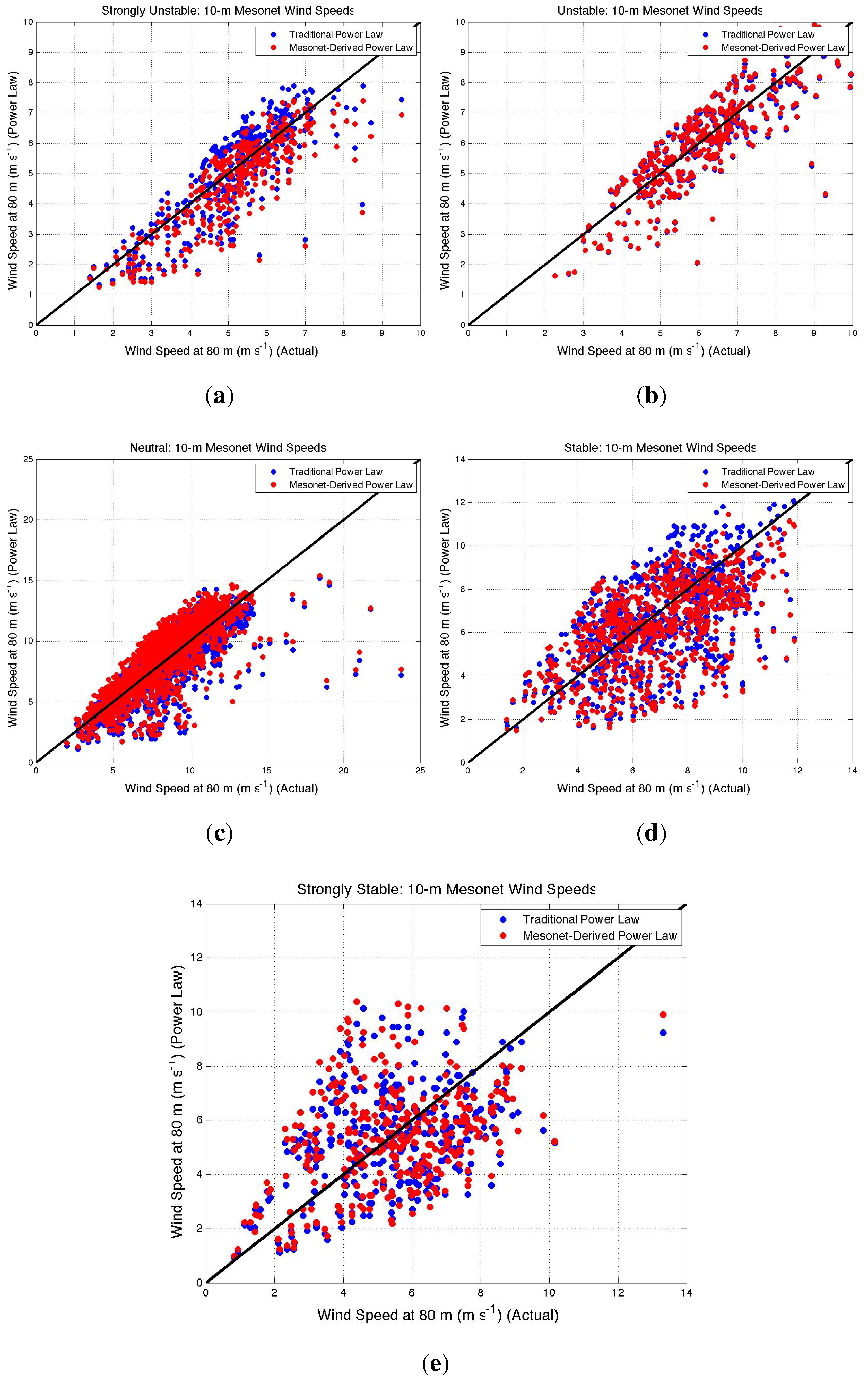
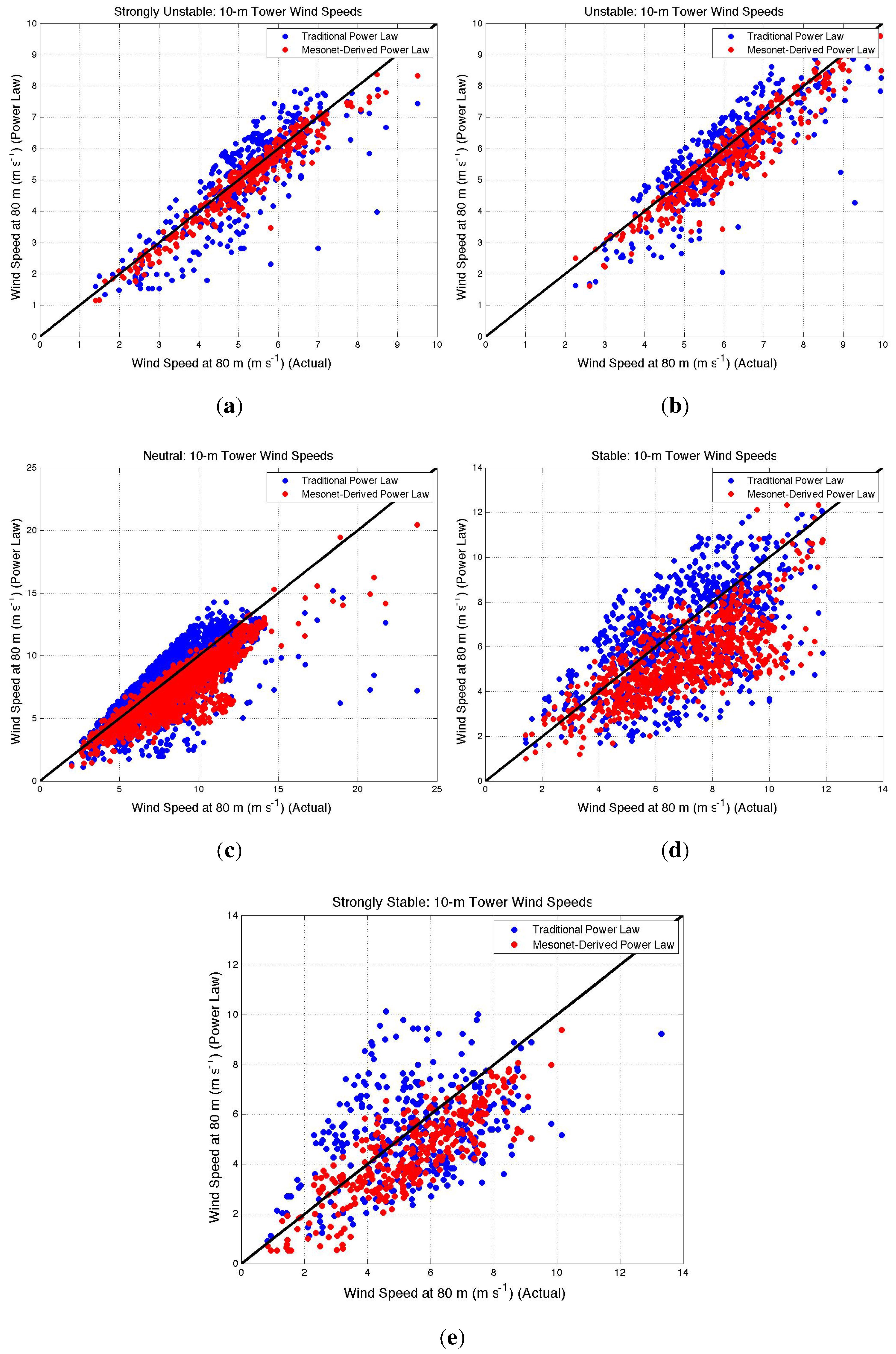
Results for the tall tower fit are not as promising; in fact, R 2 values for all stability regimes decreased when the Mesonet-derived power law fit was used, while RMSE values increased (Table 1). In order to provide greater insight into this discrepancy, scatter plots of the power law fits for both the Mesonet fit and the tower fit were examined (Figure 7 and Figure 8). The scatter about the one-to-one line is significantly reduced when tall tower 10-m wind speeds are used, leading to lower RMSE values for the power law fits in comparison to the fits that used 10-m Mesonet data (Table 1). However, the Mesonet-derived power law produced many underestimates of the true 80-m wind speed when the tower 10-m data were used, particularly for neutral and stable regimes (Figure 8 c–e). Thus, although the tall tower estimates lay closer to the one-to-one line than the Mesonet estimates on average, the slope of the tower estimates changed significantly when the Mesonet-derived power law fit was used, producing a large amount of wind speed underestimates. It is likely that this decrease in performance is the result of using stability measurements that were taken at a different location than the 10- and 80-m wind speeds. Since the Mesonet-derived power law fit depends directly on R i , the difference in stability between the Mesonet site and the tall tower site likely had a large effect on the accuracy of the shear exponent parameterization.
Figure 7. Estimated 80-m wind speeds from power law fits compared to true 80-m wind speeds for (a) strongly unstable; (b) unstable; (c) neutral; (d) stable; and (e) strongly stable regimes. Observation/estimation pairs are indicated by circles, and the 1:1 line is shown by the thick black line for reference. Data from August, 2009, were used, and Mesonet data were used for 10-m wind speeds.
Resources 03 00081 g007
Figure 8. As in Figure 7, but tower data were used for 10-m wind speeds.
Resources 03 00081 g008
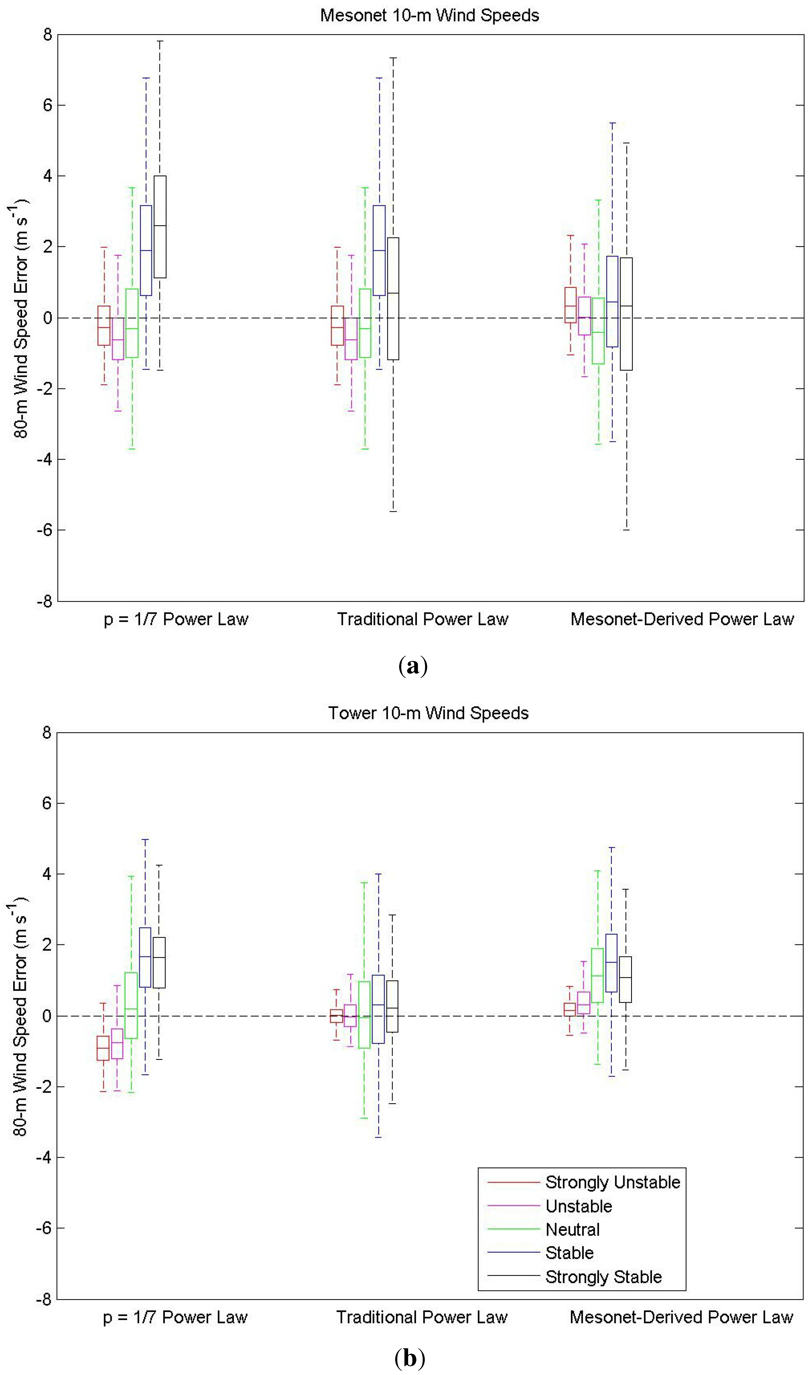
Figure 9. Box-and-whisker plots of 80-m wind speed errors for various power law extrapolation methods and stability classes. The solid line in the center of the box indicates median error; edges of the box indicate the 25th and 75th percentiles, and the ends of whiskers indicate the 10th and 90th percentiles. The black dashed line indicates an error of 0 m s - 1 . Data from August 2009, were used, and both (a) Mesonet and (b) tall tower data were used for 10-m wind speeds.
Resources 03 00081 g009
The uncertainty in the various power law extrapolation methods is depicted in Figure 9. The error was defined as the estimated 80-m wind speed subtracted from the true 80-m wind speed, such that errors above (below) the 0 m s - 1 line in Figure 9 are underestimates (overestimates) of the wind speed. For the p = 1 / 7 power law, both the Mesonet and tall tower fits produced errors near 0 m s - 1 for neutral conditions, overestimates for unstable conditions and underestimates for stable conditions. These results are expected, as the p = 1 / 7 power law is typically associated with neutral conditions. The range of expected errors decreased significantly when 10-m tall tower data were used, particularly for stable conditions.
When the traditional power law was used, the Mesonet fit tended to overestimate the wind speed for unstable and neutral conditions and underestimate the wind speed for stable conditions. The range of wind speed errors produced by the Mesonet fit is quite large for stable regimes and is likely related to the varying amounts of 10- to 80-m wind shear that occur under stable regimes. The use of tall tower 10-m wind speeds significantly improved the traditional power law fit, producing unbiased wind speed estimates for all stability classes and much smaller error ranges.
The use of tall tower 10-m wind speeds also decreased the range of errors for the Mesonet-derived power law fit. However, the median errors for the tall tower fit increased for neutral and stable regimes in comparison to the Mesonet fit, indicating that the tall tower fit tended to underestimate wind speeds for neutral and stable regimes. As previously discussed, this positive bias is likely related to the difference in stability between the Mesonet site and the tall tower site.
In summary, the use of co-located 10- and 80-m wind speeds in the power law fit methods leads to a smaller range of errors and greater certainty in the resultant wind speed estimates. However, biased estimates can be produced when stability information is collected at a different site than the 10- and 80-m wind speed data. Thus, wind speed data at 10- and 80-m, as well as stability information should be collected at the same site in order to produce wind speed estimates that are both accurate and precise.

4.3. Seasonal Effects on the Power Law Extrapolations

Next, the August, 2009, power law fits were applied to data throughout the rest of 2009 to examine the ability of the August fits to predict 80-m wind speeds during different seasons. (Only data from February to November, 2009 were used, as work was being done on the tall tower during the remaining months.) R 2 and RMSE values for the power law fits for February to November, 2009 are shown in Table 2. Even though the power law fits were only developed using one month of training data, the fits performed quite well for the remainder of the months of 2009, with all R 2 values exceeding 0.75. Similar to the training dataset, this test dataset shows a clear improvement in performance when stability information is taken into account, particularly for stable regimes (Table 2).
The accuracy of the August 2009, fits for the remainder of 2009 is significant; it indicates that hub-height wind speeds are only needed for a short period of time to develop an accurate power law fit. Thus, a wind farm could deploy a tall tower for 1–2 months to develop a representative power law fit for different stability classes, then use wind speed data from a shorter tower to estimate hub-height wind speeds for the remainder of the year. This would result in a large decrease in operation and maintenance costs for the wind farm.
Table 2. The coefficient of determination ( R 2 ) and root-mean-squared error (RMSE) values for different power law fits for all stability classes. Ten-meter wind speed data from the Mesonet and tall tower were evaluated separately to produce power law fits, and August, 2009, fits were applied to all months of data.
Month, 10-m Data SourceStrongly UnstableUnstableNeutralStableStrongly Stable
p = 1/7: R 2
February–November 2009, Mesonet0.960.970.960.870.75
February–November 2009, Tall Tower0.980.980.960.890.90
Traditional Power Law: R 2
February–November 2009, Mesonet0.960.980.960.930.87
February–November 2009, Tall Tower0.990.990.960.960.96
Mesonet-Derived Power Law: R 2
February–November 2009, Mesonet0.960.980.970.940.86
February–November 2009, Tall Tower0.990.990.960.910.94
p = 1/7: R M S E (m s - 1 )
February-November 2009-Mesonet1.21.41.92.93.1
February-November 2009-Tall Tower0.981.22.02.62.0
Traditional Power Law: RMSE (m s - 1 )
February–November 2009, Mesonet1.11.31.92.12.2
February–November 2009, Tall Tower0.500.642.01.71.3
Mesonet-Derived Power Law: RMSE (m s - 1 )
February–November 2009, Mesonet1.21.31.82.12.3
February–November 2009, Tall Tower0.580.782.22.51.6

4.4. Monin-Obukhov Similarity Theory

Similarity theory was also used as an extrapolation method as a comparison to the power law fits. Unlike the traditional power law, similarity theory is based on theories of boundary-layer fluxes and wind speed profiles and directly incorporates stability information into the extrapolation fit. However, similarity theory also contains several assumptions that may not always be true. For example, Monin–Obukhov similarity theory assumes that fluxes of heat and momentum are constant with height within the surface layer [12], an assumption that is generally untrue at night when the boundary layer is stable [27].
Similar to the process outlined for the Mesonet-derived power law fit, the gradient Richardson number was first used to calculate the similarity functions for momentum Equations (11)–(14). Next, the Obukhov length, L, was calculated by dividing z m by ζ m . Once L is known, the stability parameter, ζ, can be computed for the two measurement heights z 1 = 10 m and z 2 = 80 m. The stability correction factors at 10 and 80 m were obtained from the following generally accepted equations [12]:
Ψ m = - 5 ζ ; ζ 0
Ψ m = 2 l n 1 + x 2 + l n 1 + x 2 2 - 2 t a n - 1 ( x ) + π 2 ; ζ < 0
where x = ( 1 - 15 ζ ) 1 / 4 .
Applying Equation (2) to determine the wind speed at z 2 = 80 m requires knowledge of the friction velocity, u * , and roughness length, z o , parameters. The friction velocity, u * , was found by solving the equation for the dimensionless wind speed gradient for u * :
u * = κ z m ϕ m ( z m L ) u ¯ z
The von Kármán constant was set to 0.4, and the mean wind speed gradient was found using a finite-difference approach, assuming a logarithmic wind profile:
u ¯ z = u 10 m - u 2 m l n ( 10 m 2 m ) z m
Median values of u * were approximately 0.2–0.3 m s - 1 for all stability classes, with slightly lower values experienced during stable conditions. Next, the roughness length, z o , was calculated by applying a modified log-law profile (Equation (2)) to the wind speed at a height z 1 = 10 m and solving it for z o :
z o = 10 m × e x p - κ * u ( 10 m ) u * - Ψ m ( ζ 1 )
Median values of z o derived from the data were approximately 0.01 m for the month of August, 2009, which is fitting for the open fields near the Cheyenne Mesonet site [28]. Finally, the calculated values of u * , z o and Ψ m ( 80 m ) were used to calculate the wind speed at 80 m from the modified log-law equation (Equation (2)).
The R 2 and RMSE values for the MOST method are shown in Table 3 for February to November, 2009 (Note that the Monin–Obukhov method assumes a maximum R i of 0.2, so similarity theory was not applied to the strongly stable regime wind speeds or stable regime wind speeds where R i 0 . 2 ). Similar to the power law method, more accurate fits were produced for the unstable regime wind speed pairs, consistent with previous work (e.g., [20]). In general, the MOST method performed much more poorly for the stable regime wind speeds in comparison to the power law method.
To provide insight into this discrepancy, scatter plots of the 80-m wind speeds estimated from MOST were examined for different stability regimes (not shown). Similarity theory produced fairly good results for the strongly unstable, unstable and neutral regimes using both 10-m datasets ( R 2 > 0.9); the observation/estimation pairs were scattered somewhat uniformly about the 1:1 line, indicating that similarity theory produced approximately equal numbers of overestimates and underestimates of the 80-m wind speed. However, many of the similarity theory estimates were inaccurate for the stable regime, with a large scatter above the one-to-one line ( R 2 = 0.50, RMSE = 5.9 m s - 1 for the tower fit). Thus, MOST appears to be overestimating the amount of wind shear between 10 and 80 m for stable conditions, consistent with the findings of Holtslag [20]. This poor performance for stable regimes is not surprising; it is likely that 80 m is above the top of the surface layer for stable conditions, invalidating the application of MOST at 80 m. Indeed, based on data from the Wangara experiment, Hicks [29] found that the wind speed profile under very stable conditions eventually transitions from a log-linear profile to an approximately linear profile, deviating substantially from the profile predicted by MOST.
Table 3. The coefficient of determination ( R 2 ) and the root-mean-squared error (RMSE) values for MOST and Extended Monin–Obukhov Similarity Theory (EMOST) for different datasets and stability classes.
Month, 10-m Data SourceStrongly UnstableUnstableNeutralStable
Monin-Obukhov Similarity Theory: R 2
February–November 2009, Mesonet0.950.970.950.47
February–November 2009, Tall Tower0.990.990.970.50
Extended Monin-Obukhov Similarity Theory: R 2
February–November 2009, Mesonet0.940.970.950.85
February–November 2009, Tall Tower0.990.990.950.88
Monin-Obukhov Similarity Theory: RMSE (m s - 1 )
February–November 2009, Mesonet1.31.32.36.0
February–November 2009, Tall Tower0.520.701.75.9
Extended Monin-Obukhov Similarity Theory: RMSE (m s - 1 )
February–November 2009, Mesonet1.41.42.33.3
February–November 2009, Tall Tower0.640.782.43.0
In order to improve the application of similarity theory for stable regimes, the extended Monin–Obukhov similarity theory method of Gryning et al. [21] was also used to estimate 80-m wind speeds. By using different length scales for different parts of the boundary layer, Gryning et al. [21] show that the wind speed profile in neutral conditions can be determined through the following equation:
u ¯ ( z ) = u * κ l n z z o + z L M B L , N - z z i z 2 L M B L , N
L M B L , N is the length scale in the middle boundary layer under neutral conditions. By using tower observations, Gryning et al. [21] determined an empirical fit for L M B L , N , given by:
L M B L , N = u * o f / ( - 2 l n u * o f z o + 55 )
where f is the Coriolis parameter.
The general form of the wind profile is given by Equation (4), where Ψ m is a stability correction factor. For stable conditions, Gryning et al. [21] suggest Ψ m = b z L ( 1 - z 2 z i ) . In this work, the constant, b, was set to five, following the relations outlined in Arya [12]. For unstable conditions, Gryning et al. [21] suggest Ψ m = 3 2 l n 1 + x + x 2 3 - 3 t a n - 1 ( 1 + 2 x 3 ) + π 3 , where x = ( 1 - 12 z / L ) 1 / 3 . For both stable and unstable conditions, Gryning et al. [21] determined the following empirical relation for L M B L :
L M B L = u * o f / [ ( - 2 l n u * o f z o + 55 ) e x p ( - u * 0 / f L 400 ) ]
Previously calculated values of u * and z o , determined using the MOST method, were used in the EMOST equations. Gryning et al. [21] used a similar method to estimate z o by forcing the estimated wind profile to coincide with the measured wind speeds at 10 m. However, Gryning et al. [21] were able to calculate u * directly with sonic anemometer data instead of estimating u * from the dimensionless wind speed gradient equation (Equation (21)).
One of the parameters in the EMOST wind profile equations is the boundary layer height, z i . Gryning et al. [21] estimate the mean boundary layer height for different stability regimes by examining heat and momentum fluxes from sonic anemometers on a tower and extrapolating the flux measurements upward. However, sonic anemometers are not available on either the tall tower or the Mesonet station, so a simple parameterization for the boundary layer height was used in this paper. Gryning et al. [21] suggest that the approximation z i 0 . 1 u * o /f be used when the boundary layer height is not known, so this approximation was adopted for the present study.
R 2 values for the EMOST method are shown in Table 3. (Again, the application of EMOST was restricted to cases where R i < 0 . 2 .) Similar to the MOST estimates, the 80-m wind speed estimates from EMOST were most accurate for strongly unstable, unstable and neutral regimes. However, the EMOST wind speed estimates for stable regimes are significantly closer to the observed 80-m wind speeds (e.g., R 2 = 0.88 using tower 10-m data) in comparison to the MOST estimates ( R 2 = 0.50 for the same dataset). In addition, unlike the MOST estimates, the EMOST wind speed estimates are scattered more uniformly about the one-to-one line, indicating that both overestimates and underestimates of the 80-m wind speed are produced (not shown). Thus, there does seem to be a slight advantage to using the extended Monin–Obukhov Similarity Theory of Gryning et al. [21], at least for stable regime wind speed estimates. However, both the traditional and Mesonet-derived power law fits generally produced more accurate extrapolation results for all stability regimes in comparison to the similarity theory methods (Table 2 and Table 3). In addition, the power law fits did not require the estimation of parameters such as friction velocity and boundary layer height.
5. Summary and Conclusions

In this work, 10-m wind speed data from the Cheyenne Mesonet site and 10- and 80-m wind speed data from a nearby tall tower were used to evaluate different wind speed extrapolation techniques. A standard p = 1 / 7 power law, a traditional power law, a Mesonet-derived power law and two different forms of similarity theory were evaluated for different stability classes. The main findings from the various methods can be summarized as follows:
  • Both the traditional power law and the Mesonet-derived power law improved upon the p = 1 / 7 neutral power law fit, indicating that stability information should be used to produce more accurate extrapolation fits;
  • All power law fits were significantly improved when tower 10-m wind speed data were used;
  • Wind speed estimate biases were produced for the Mesonet-derived power law method when stability information and 10- and 80-m wind speed data were collected at two different locations;
  • Similarity theory methods only produce accurate wind speed estimates for unstable conditions;
  • Overall, the power law fits produced the most accurate 80-m wind speed estimates;
  • Power law fit parameters developed from one month of data (August) can be applied to wind speed data from different time periods (the remainder of the year) to produce accurate wind speed estimates
In the future, the performance of the Mesonet-derived power law fit could be improved by examining the dependence of the neutral shear exponent on wind direction and upwind fetch. In addition, the performance of the power law methods could likely be greatly improved by having co-located stability data and hub-height wind speed information. However, the stability information derived from a Mesonet site could still be used to produce accurate power law fits for a nearby tall tower. This stability information significantly increased the accuracy of extrapolation methods in comparison to the traditional p = 1 / 7 power law fit.

Acknowledgments

The authors would like to thank Michael Klatt at the Oklahoma Wind Power Initiative for his assistance in obtaining tall tower data.

Conflicts of Interest

The authors declare no conflict of interest.

References

  1. United States Energy Information Administration. Annual Energy Outlook 2012. Available online: http://www.eia.gov/forecasts/aeo/pdf/0383(2012).pdf (accessed on 1 July 2013).
  2. United States Department of Energy. 20% Wind Energy by 2030: Increasing Wind Energy’s Contribution to U.S. Electricity Supply. Available online: http://www.nrel.gov/docs/fy08osti/41869.pdf (accessed on 1 July 2013).
  3. Schwartz, M.; Elliott, D. Towards a Wind Energy Climatology at Advanced Turbine Hub-Heights. In Proceedings of the 15th Conference on Applied Climatology, Savannah, Georgia, USA, 20 June 2005.
  4. Petersen, E.L.; Mortensen, N.G.; Landberg, L.; Højstrup, J.; Frank, H.P. Wind power meteorology. Part II: Siting and models. Wind Energy 1998, 1, 55–72. [Google Scholar] [CrossRef]
  5. Del Franco, M. Remote sensing equipment comes of age. N. Am. Wind Power 2012, 9, 36–38. [Google Scholar]
  6. U.S. Department of Energy. Utility-Scale Land-Based 80-Meter Wind Maps. Available online: http://www.windpoweringamerica.gov (accessed on 15 January 2014).
  7. Petersen, E.L.; Mortensen, N.G.; Landberg, L.; Højstrup, J.; Frank, H.P. Wind power meteorology. Part I: Climate and turbulence. Wind Energy 1998, 1, 25–45. [Google Scholar] [CrossRef]
  8. Smedman-Högström, A.S.; Högström, U. A practical method for determining wind frequency distributions for the lowest 200 m from routine meteorological data. J. Appl. Meteor. 1978, 17, 942–954. [Google Scholar] [CrossRef]
  9. Irwin, J.S. A theoretical variation of the wind profile power-law exponent as a function of surface roughness and stability. Atmos. Environ. 1979, 13, 191–194. [Google Scholar] [CrossRef]
  10. Zoumakis, N.M. The dependence of the power-law exponent on surface roughness and stability in a neutrally and stably stratified surface boundary layer. Atmósfera 1993, 6, 79–83. [Google Scholar]
  11. Van den Berg, G.P. Wind turbine power and sound in relation to atmospheric stability. Wind Energy 2008, 11, 151–169. [Google Scholar] [CrossRef]
  12. Arya, S.P. Introduction to Micrometeorology, 2nd ed.; International Geophysics Series; Academic Press: Cornwall, UK, 2001; Volume 79. [Google Scholar]
  13. Kaimal, J.C.; Finnigan, J.J. Atmospheric Boundary Layer Flows: Their Structure and Measurement; Oxford University Press: New York, NY, USA, 1994. [Google Scholar]
  14. World Meteorological Organization. WMO Guide to Meteorological Instruments and Methods of Observation. Available online: www.nrel.gov/docs/fy08osti/41869.pdf (accessed on 25 November 2013).
  15. McPherson, R.A.; Fiebrich, C.A.; Crawford, K.C.; Kilby, J.R.; Grimsley, D.L.; Martinez, J.E.; Basara, J.B.; Illston, B.G.; Morris, D.A.; Kloesel, K.A.; et al. Statewide monitoring of the mesoscale environment: A technical update on the Oklahoma Mesonet. J. Atmos. Ocean. Technol. 2007, 24, 301–321. [Google Scholar] [CrossRef]
  16. Oklahoma Wind Power Initiative. Available online: http://www.ocgi.okstate.edu/owpi (accessed on 15 January 2014).
  17. Wagner, R.; Antoniou, I.; Pedersen, S.M.; Courtney, M.S.; Jørgensen, H.E. The influence of the wind speed profile on wind turbine performance measurements. Wind Energy 2009, 12, 348–362. [Google Scholar] [CrossRef]
  18. Emeis, S.; Harris, M.; Banta, R.M. Boundary-layer anemometry by optical remote sensing for wind energy applications. Met. Zeit. 2007, 16, 337–347. [Google Scholar] [CrossRef]
  19. Garratt, J. The Atmospheric Boundary Layer; Cambridge Atmospheric and Space Science Series; Cambridge University Press: Cambridge, UK, 1992. [Google Scholar]
  20. Holtslag, A.A.M. Estimates of diabatic wind speed profiles from near-surface weather observations. Bound. Lay. Meteorol. 1984, 29, 225–250. [Google Scholar] [CrossRef]
  21. Gryning, S.E.; Batchvarova, E.; Brümmer, B.; Jørgensen, H.; Larsen, S. On the extension of the wind profile over homogeneous terrain beyond the surface boundary layer. Bound. Lay. Meteorol. 2007, 124, 251–268. [Google Scholar] [CrossRef]
  22. Klatt, M. D.; University of Oklahoma, Norman, OK, USA. Personal communication, 2013.
  23. Bodine, D.; Klein, P.M.; Arms, S.C.; Shapiro, A. Variability of surface air temperature over gently sloped terrain. J. Appl. Meteor. Climatol. 2009, 48, 1117–1141. [Google Scholar] [CrossRef]
  24. Mauritsen, T.; Svensson, G. Observations of stably stratified shear-driven atmospheric turbulence at low and high Richardson numbers. J. Atmos. Sci. 2007, 64, 645–655. [Google Scholar] [CrossRef]
  25. Wharton, S.; Lundquist, J.K. Assessing atmospheric stability and its impacts on rotor-disk wind characteristics at an onshore wind farm. Wind Energy 2012, 15, 525–546. [Google Scholar] [CrossRef]
  26. Panofsky, H.A.; Blackadar, A.K.; McVehil, G.E. The diabatic wind profile. Quart. J. Roy. Meteor. Soc. 1960, 86, 390–398. [Google Scholar] [CrossRef]
  27. Pahlow, M.; Parlange, M.; Porté-Agel, F. On Monin–Obukhov similarity in the stable atmospheric boundary layer. Bound. Lay. Meteorol. 2001, 99, 225–248. [Google Scholar] [CrossRef]
  28. Stull, R.B. Meteorology for Scientists and Engineers, 1st ed.; Brooks Cole: Dordrecht, The Netherlands, 1988. [Google Scholar]
  29. Hicks, B.B. Wind profile relationships from the “Wangara" experiment. Quart. J. Roy. Meteor. Soc. 1976, 102, 535–551. [Google Scholar]