Article

Enhancement of a District Heating Substation as Part of a Low-Investment Optimization Strategy for District Heating Systems

Institute of New Energy Systems, University of Applied Sciences Ingolstadt, Esplanade 10, D-85049 Ingolstadt, Germany
*
Author to whom correspondence should be addressed.
Resources 2021, 10(5), 53; https://doi.org/10.3390/resources10050053
Submission received: 29 March 2021 / Revised: 11 May 2021 / Accepted: 12 May 2021 / Published: 19 May 2021

Abstract

:
In an ongoing project, low-investment measures for the optimization of district heating systems are analyzed. The optimization strategies are collected in a catalog, which is the core of a guideline. The application of this guideline is demonstrated using two concrete district heating networks as examples. In this study, the improvement of an analog controlled district heating substation by an electronic controller is investigated. High supply temperatures and heat losses are often a challenge in district heating networks. The district heating substations have a major influence on the network return temperatures. The comparison of the two substation setups with analog and electronic controllers is carried out by laboratory measurement. It can be shown that the return temperatures can be reduced by an average of 20 K in winter and transition, as well as 16 K in summer. The district heating network losses are calculated for one of both specific district heating networks. They are calculated from the ratio of network losses to generated energy. The generated energy is the sum of network losses and consumer demand. The thermal losses of the network can be reduced by 3%. The volume flow in the heating network can be reduced to a quarter. Therefore, the pumping energy requirement drops sharply since these changes cubically affect the volume flow.

1. Introduction

The presented study is in the context of the transformation of existing district heating networks (DHNs) into so called fourth generation DHNs’ [1]. Some studies have described this transformation [2,3]. This transformation ensures the continued existence of DHNs in the future, as it aims for lower heat losses and allows the integration of low-temperature heat into DHNs, such as renewable-energy based heat sources or industrial excess heat. Sorknæs et al. [4] demonstrated the economic and energetic effect from third to fourth generation transition by considering Aalborg Municipality, Denmark as a case study area. The cost of the energy system was reduced by about 3%, and total primary energy demand was reduced by 4.5%, which was achieved as a result of the better integration of industrial waste heat and heat pumps to DHNs. Averfalk and Werner [5] pointed out that in the case of heat generation from geothermal energy, industrial excess heat, solar thermal energy and heat pumps, the influence of lower network temperatures on heat generation costs is distinctive.
Since lower network temperatures are a necessary prerequisite in order to use the aforementioned heat sources, various optimization approaches were investigated to reduce the return temperatures in DHNs. Table 1 summarizes the various optimization measures and their impact in order to reduce the return temperatures.
Basciotti et al. [6] investigated the influence of building renovation on the reduction of return temperatures. However, only a significant retrofitting rate (more than 80% of the buildings in the studied area) helped to bring down return temperature in the DHN up to 1.2 °C. Köfinger et al. [7] examined the reduction by supplying new consumers with low system temperatures from the return flow of existing consumers with high system temperatures. In that scenario, consumers with a total heat demand of 630 MWh were connected to an existing heating network with an annual demand of 2400 MWh. In this study, the return temperature could be reduced by 1.8 °C.
Other developments have revealed, including that both the optimal operation of the space heating system and the control strategy of the district heating substation (DHS) can positively contribute to an improvement of the overall efficiency. A new control method investigated by Gustafsson et al. [8] compared the previous heating control (based on the outdoor temperature) with a methodology that takes the primary supply temperature of the network into account. A larger temperature difference between flow and return was achieved by the control algorithm compensating for the variation in the outdoor temperature and the fluctuations in the supply temperature on the network side. The return temperature could be reduced by a maximum of up to 4.8 °C. Optimal control was developed for the consumer-side heating supply temperature and volume flow by van Oevelen et al. [9]. The secondary supply temperature was increased with a simultaneous reduction of the secondary volume flow. Using this method, the average return temperature in the high-temperature case dropped by 6 °C. The authors also investigated the impact of oversized heating system design. They identified that with 100% oversizing, the return temperature can be decreased by 9.8 °C. Both measures together led to reductions in the return temperature of up to 18.2 °C. Tol et al. [10] developed a control strategy that allowed for the adoption of the feed temperature at the district level to the cooling performance of the consumer substation. Compared to the outside temperature-based control strategy, the new one led to less electricity power loss in the case of the cogeneration heat and power plant.
In order to increase the efficiency of DHNs, faults in customer stations have to be identified. A new fault detection method has been presented which works with the temperature difference signature [11]. The method presented is fast and inexpensive, and therefore feasible in practice. A field test in a Swedish district showed that 10% of substations were identified with temperature difference faults by on-site inspection, while 6% were detected by this method. Another method to identify faults in DHS is excess flow analyses [12]. Testing this method in the field estimates a return temperature reduction of 4 °C to 8 °C, even though only typical errors such as calcified heat exchangers and missing check valves are fixed. Since reliable fault detection brings so much savings, research is being conducted on various approaches [13].
Table 1. Methods for lowering return temperatures.
Optimization MeasureDecreased Return TemperaturesReference
Retrofitting buildings1.2 °C[6]
High- and low-temperature consumer cascade1.8 °C[7]
Heating supply temperature controlled by DHN feed temperature4.8 °C[8]
Heating control curves6 °C[9]
Oversizing heating system design9.8 °C[9]
Faulty detection of DHS and elimination of typical faults in DHS4 °C to 8 °C [12]
The optimization of the design and hydraulics is also still progressing. In references [14,15], various DHS constructions were identified for multifamily buildings in order to reduce the DHN return temperatures. A promising concept with a fresh water module and a serial-connected heat exchanger led to better cooling and has been described as economically feasible [14]. Elfner et al. [16,17] further developed the aforementioned concept for different heat generation plants, as well as building types and standards. In doing so, the return temperatures can be reduced and therefore the efficiency of the overall system can be significantly improved. For single-family houses (SFHs), the financial framework is too tight for more complex DHS systems. Therefore, the design of the DHS needs to be implemented by only a few components. The presented study shows that return temperatures can be reduced by 16 °C to 20 °C by means of an electronic controller with less expense. The study aims to show that a fundamental upgrade of the analogue standards in existing DHNs should always be considered. Since in these cases the DHN feed temperature is maintained, the capacity of the system is increased considerably so that further consumers can be connected. Otherwise, the volume flow drops profitably.
The results of this study will be transferable to a whole range of DHNs. Analog controlled DHSs with so called self-operated valves are quite common [18]. Between the end of the 1990s and the 2020s, more DHNs were built in Germany using the heat generated from the biomass combined heat and power process. The heat extracted from biomass cogeneration was often seen as a costless supplement to electricity generation. Therefore, the focus was not on heat use efficiency. With the ending of the Renewable Energies Act (EEG) subsidy after 20 years of operation, the focus is now shifting to the efficient use of heat. Therefore, this study will help some DHN operators to continue operating their DHNs more economically.

2. Materials and Methods

2.1. Positioning of This Study in the Overall Context of the OREWA Project

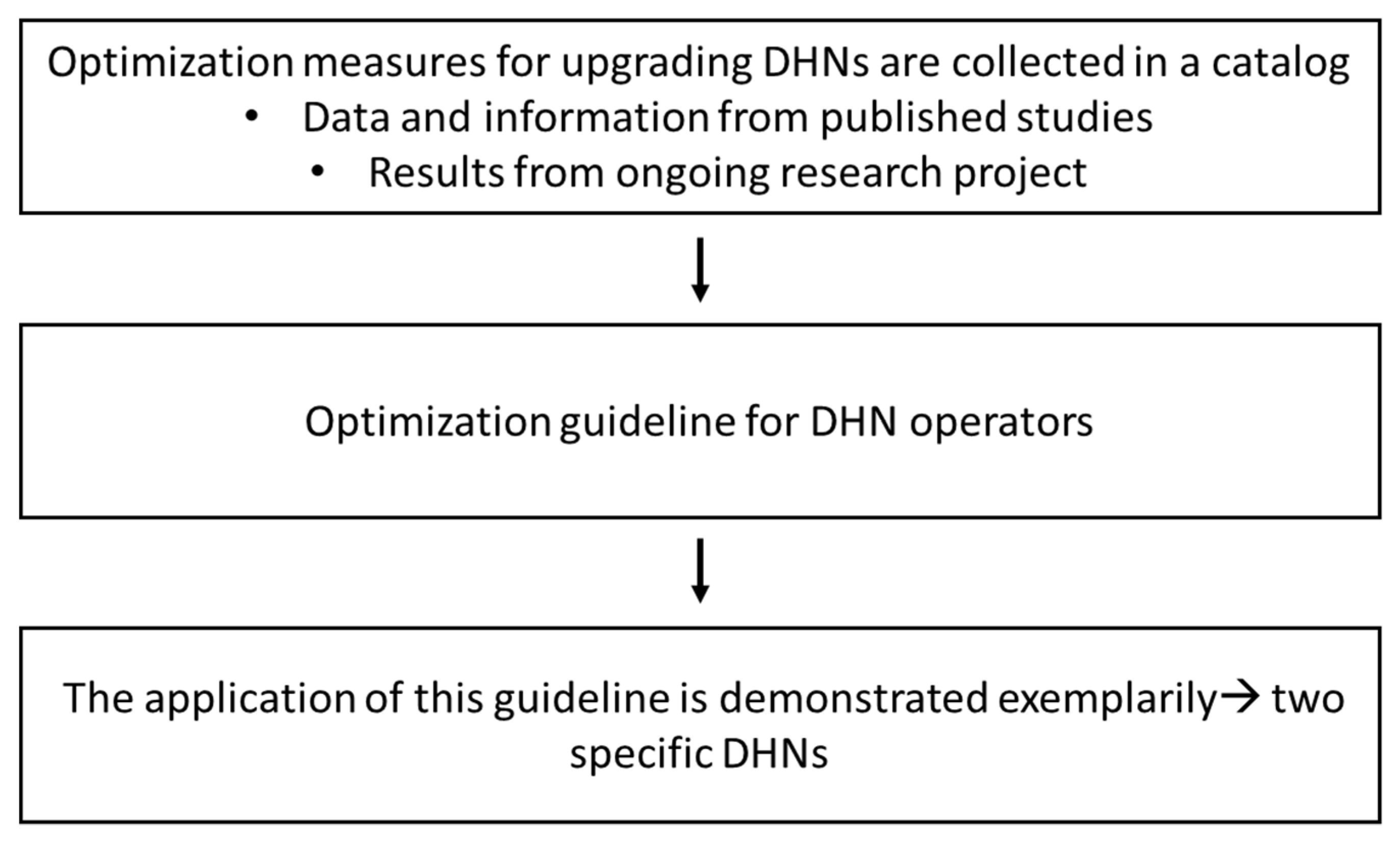
Improving DHNs with low-investment measures ensures their cost- and energy-efficient operation in the future and is vital for energy transition. The ongoing research project ‘OREWA’ (optimization and restructuring of DHNs including evaluation of transferability, ecology, and economy) contains the collection of optimization measures in a catalog up to the application of these measures. The three methodical steps are illustrated in Figure 1.
The first step of the OREWA project shown in Figure 1 involves collecting optimization measures from published studies and from the ongoing investigation. The catalog is intended to serve as a guideline for district heating operators. Based on typical DHN characteristics such as overall energy demand, heat density, network temperatures or key performance indicators like those defined in [19], the measures are extracted that can be useful and economical for a specific network. Thus, in the second step (cf. Figure 1), a selection process is implemented. The measurements which are identified to be sensible must be examined more closely for the operator’s DHN. This procedure will be demonstrated in the third step using two exemplary DHNs.
Within the third step, the presented investigation is to be placed, and the step will be shown exemplarily. For the specific DHNs, several measures from the catalog are eliminated because of their specific characteristics. The DHNs are small and have high heat losses and high DHN return temperatures. Therefore, the measures identified as beneficial are the upgrade of the substations and subsequently the reduction of the return temperatures. This paper focuses on the laboratory experiment used to determine the potential optimization of the DHS and thus for the district heating system. The results are then used to calculate the thermal savings via simulation. In addition, the cost of improving the substation must be calculated accurately.

2.2. Objective of DHS Optimization

Analysis of the specific DHNs showed that the difference between the supply and return temperatures of the DHNs is about 8 K on an annual average. Thus, the system is very inefficient. It was recognized that this is due to the analog controlled DHSs with so called self-operated valves. It was observed that high volume flows continuously flowed on the primary side of the substation, even in times with no demand. On the one hand, the everlasting volume flow is due to the kind of the controller; on the other hand, the high-volume flows are due to poor manual adjustment of the controller. The question is how to lower the return temperatures and enhance the controller. For this purpose, a few necessary requirements were considered for the new DHS controller:
  • It should need as few parameters as possible and can be installed into the existing DHS;
  • It should be built as a retrofitting module for each analog controlled existing DHS;
  • It should be as simple and therefore inexpensive as possible;
  • It should close the valve on the DHN side completely in times with no demand;
  • It should be able to control the supply temperature on the heating system side. Thus, the return temperature will be lower, because the heating systems need only 60 °C for the supply temperature and not 70 °C, which is automatically set with the analog controller (see detailed description below);
  • It should have a communication interface to the heating center. Firstly, this enables faults to be detected and secondly, further optimization, such as intermittent operating strategies, can be implemented.
Basically, the electronic controller requires two values for the valve opening degree (cf. Figure 2b red circled valve). One is the maximum acceptable return temperature on the DHN side TDHN return limit and the other is the desired supply temperature on the secondary side Ttarget sec. supply. The actual values of TDHN return and Tsec. supply are compared with the specified temperatures. Figure 3 displays the controller logic which is used to operate the primary side valve.

2.3. Description of the State-of-the-Art and Optimized DHS Setup

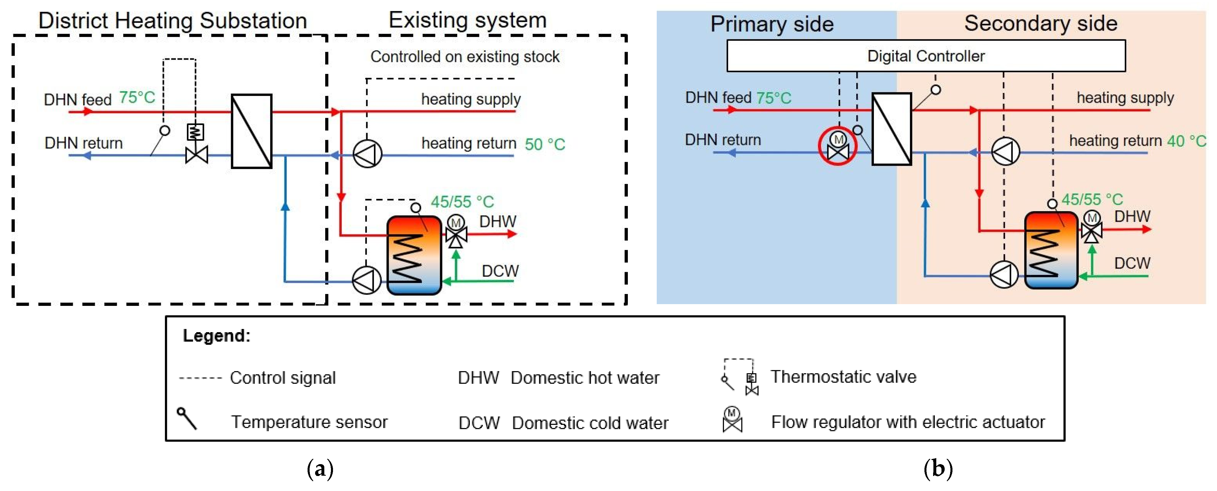
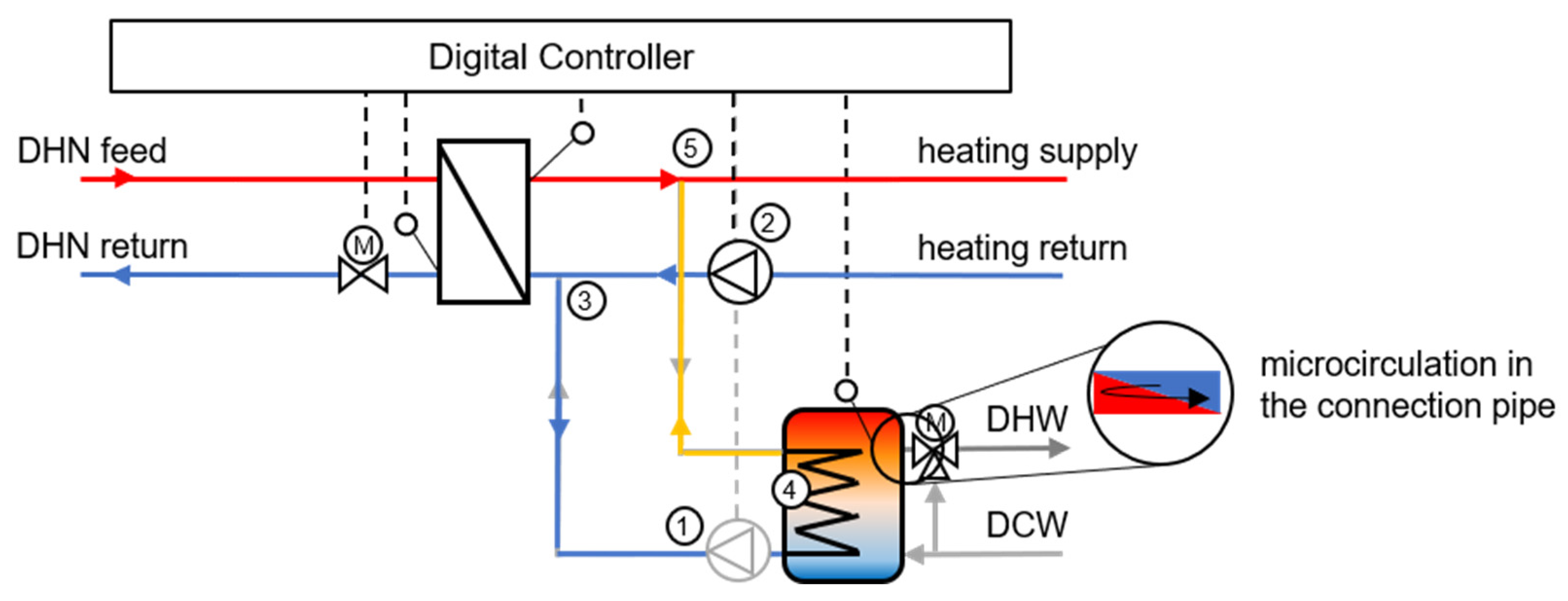
The DHS, which is installed in the two specific networks, is shown in Figure 2a. The part of the DHS setup from the DHN to heat exchanger is called the primary side. The domestic installation is referred to as the secondary side. Originally, the heating systems in such SFHs were supplied by oil boilers. By removing these oil boilers, the domestic hot water (DHW) storages, as well as the controllers of the pumps, were left independent from the new heat transfer components. In principle, the DHN is coupled into the existing house system via a plate heat exchanger and a thermostatic valve. The thermostatic valve is set to a target return temperature on the primary side (cf. Figure 2a). Fluid between the sensor and the valve expands to a greater or lesser extent proportionally to the DHN return temperature and thus determines the degree of opening of the valve. In the case of a low temperature in the DHW return pipe, the consumption by the consumer is assumed to be high. Subsequently, the fluid within the thermostat sensor contracts, allowing the valve to open further. If the demand is small or non-existent, i.e., the DHN return temperature is close to the DHN feed temperature, the valve almost closes completely. A permanent small opening of the valve is necessary for the proper functioning of the thermostatic valve. However, this leads to the fact that during times of low heat demand (e.g., summer), a small mass flow with high temperature permanently flows through the pipes, causing high thermal losses of the DHN. The thermostat DHS is an ‘uncontrolled DHS’, as the secondary side cannot be set to specific set points. As a result, the temperature on the secondary side solely depends on the temperature on the primary side.
To overcome the aforementioned problems, the thermostatic valve is replaced by a flow controller with an additional electric actuator (cf. Figure 2b, red circled valve).
The automatic flow controller can be configured individually in each SFH to meet the maximum load agreed in the contract with the network operator. Configuration of the automatic flow controller allows for easier hydraulic balancing of the DHN. The particular advantage of this method is that the DHN can properly supply all consumers in the design case; even the consumers at the furthest point from the heating center receive the ordered power. In combination with the electric actuator, an electronic controller controls the flow. The required parameters are stored in the controller. Another advantage of the electronic controller is that central control from the heating center is possible. Depending on the given parameters, the controller can adjust the flow by means of the electric actuator. In case of no consumption, the valve is completely closed, therefore reducing the thermal losses of the DHN. At the same time, it is possible to separate the supply of the space heating system from charging the DHW storage. The particular advantage of such a DHW charging priority is that the storage tank can be charged as quickly as possible. The maximum load can be used for charging the storage tank. During the time when the storage tank is charged, the return temperatures are much higher than at times when only the heating is operated. Thus, a fast charging time keeps the time with high return temperatures as short as possible. This system is undoubtably more complex than the uncontrolled one. The electronic control requires a few settings, and the valve is dependent on auxiliary power.
To quantify the benefit of this setup, both DHSs were measured on a thermal test rig in the laboratory (cf. Figure 4).
In the subsequent text, the following abbreviations are used for the systems:
  • Thermostatically controlled DHS (ThermDHS);
  • Electronically controlled DHS (ElecDHS).
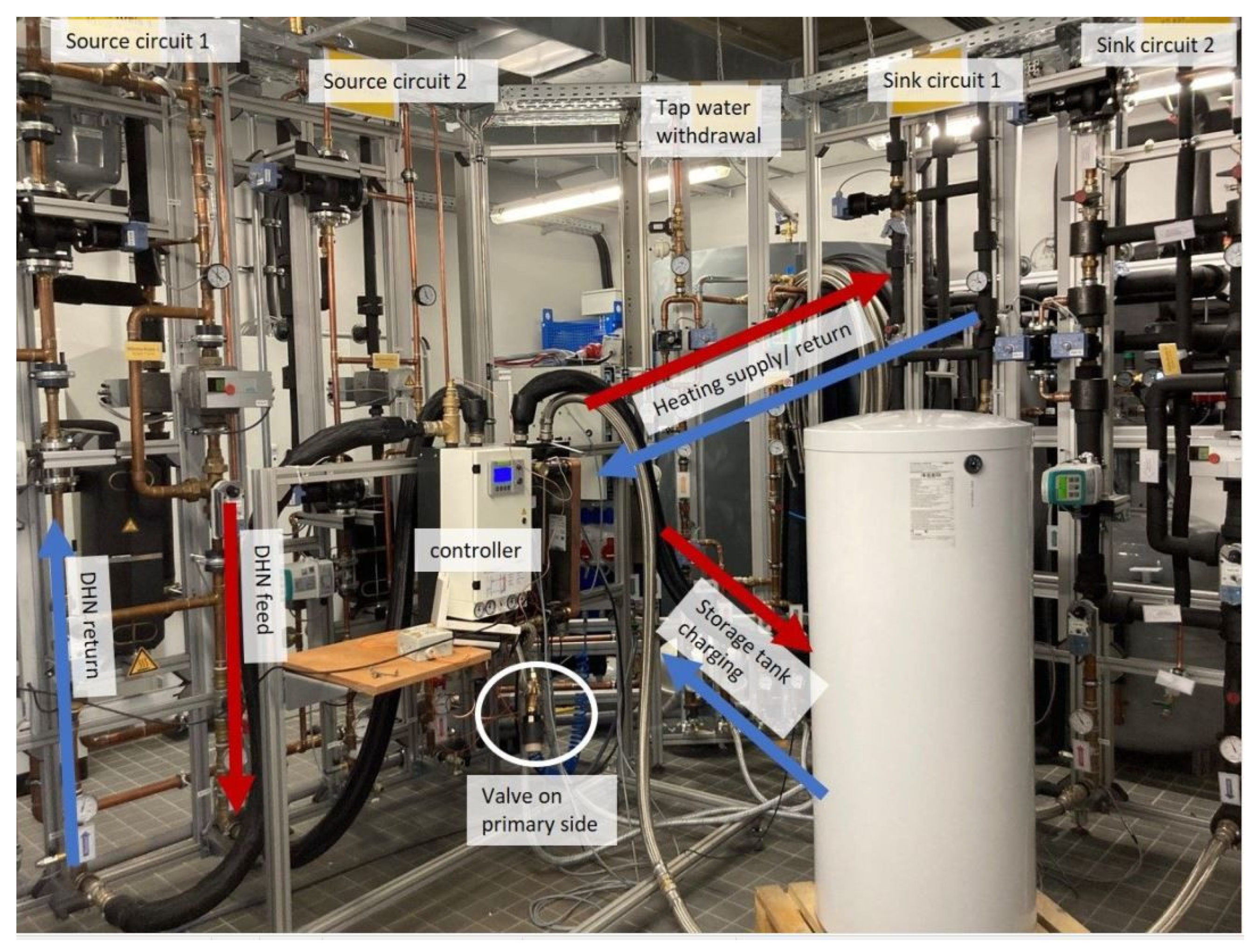
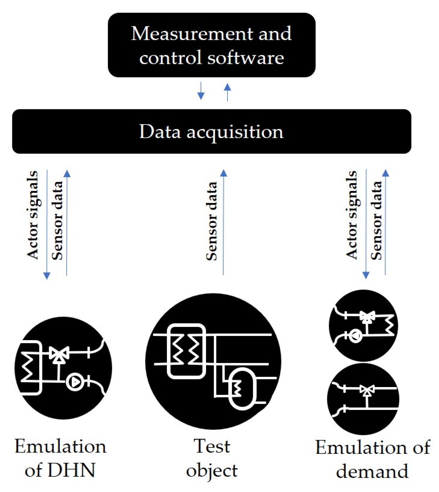
The investigation was carried out by measurements in the laboratory. For this purpose, a thermal test rig was constructed (cf. Figure 5). All sensors and actuators were controlled and measured by software. Data acquisition devices connect the software and the hydraulic circuits. They transmit the values to the actuators and record the values from the sensors. The DHN, as well as the heating and tap water demand, are emulated with the hydraulic circuits of the test rig [20].
The measurement of both DHSs takes place under the same consumer demand profiles. They are measured under a representative heating load profile of a winter day and a transition day [21]. In the case of the DHW demand, the same profile is used for winter, transition, and summer days. The measurement of each typical day means a 24 h measurement. The resolutions of the load profiles should be chosen in such a way that they provoke a realistic behavior of the DHS. Therefore, the resolutions worked out by [14] were chosen (cf. Table 2). A data acquisition unit recorded the measurement data every 2 s. This ensures that peaks are detected as accurately as possible.
The three measured typical days are used to calculate the values like return temperatures or DHN losses for one year (cf. Section 3.4.2).
In order to use representative load profiles, the heating profiles according to VDI 4655 were utilized [21]. The annual heating demand was determined from the typical demands (cf. Table 3).
For the DHW demand profiles, a load profile with a high resolution was used (cf. Table 2). In the case of the two investigated DHNs, an average of 3.4 people live in a household, which results in an average daily demand of 4.7 kWh. The values used as a basis for calculating the DHW demand are shown in Table 4.
The temperature levels given in Table 5 were used as the basis for the measurements in the laboratory. The specific DHNs are both operated with constant supply temperatures of 75 °C all year round. A heating system design temperature of 60 °C/40 °C is representative of the consumers in both existing DHNs according to the operator. However, the disadvantage with the ThermDHS is that the secondary side supply temperature cannot be determined. It depends directly on the DHN feed temperature. Thus, the supply temperature on the secondary side for this system is 70 °C.
The heat demand profiles were calculated for measurement in the laboratory with a constant supply and return temperature. As described, these are 60 °C/40 °C for the ElecDHS and 70 °C/50 °C for the ThermDHS. Accordingly, the volume flows vary depending on the fluctuating demand.
In DHNs, a low maximum charging temperature of the storage tank is typically aimed for, as the return temperatures rise accordingly during charging. At the same time, lower charging temperatures can keep the calcification of the heat exchanger low [14]. Therefore, 55 °C was used as the maximum storage temperature in the laboratory test. At this operating temperature, [23] requires that the water be completely replaced at least every three days. In practice, however, to prevent legionella, the DHW storage tanks are designed to replace the water once a day. With the electronic controller, however, the once-a-day heating up to and over 60 °C can also be fulfilled. The temperature sensor is located at one-third of the way below the top of the storage tank. In the laboratory test, the storage tank in the DHS has a volume of 200 L.
With the ElecDHS, the storage tank can be charged with priority. This means that the heating is off when the storage tank is charged. As a result, the supply temperature on the secondary side can be controlled independently from the supply temperature when the heating system is in operation.
As an outcome of the presented article, the energetic benefit of reducing the return temperatures is calculated for one of the two specific DHNs. Considering the energy demand of the circulation pump allows for an extrapolation of the electrical energy savings.

3. Results and Discussion

3.1. Quality of Measurement Data

To ensure sufficient quality of the measurement data, the same boundary conditions must be met during the measurement. This includes that the constant supply temperature on the primary side of 75 °C for the DHN emulation is met, as well as that the temperature decrease in the heating circuit corresponds to the setpoint of 40 °C in case of ElecDHS and 50 °C in case of ThermDHS. All target temperatures are colored green in Figure 2. Likewise, the heating and DHW energy quantities purchased must correspond to the target values. The relative errors ( δ x ) describe the deviation from the target values (cf. Figure 6), which are calculated according to Equation (1) [24].
T r e t u r n , n = i n ( T r e t u r n , i × m ˙ r e t u r n , i ) i n m ˙ r e t u r n , i
The measured and target values for the heating energy demand differ because the target value for heating energy demand was calculated with a specific temperature difference. In practice, the temperature difference between the supply and return temperatures is slightly off. The deviations have not influenced the evaluated return temperature. It has a negligible impact on the required mass flow from the heating network. The measurement data can be validly compared.

3.2. Resulting Return Temperatures

The pure measured values are not compared, since the mass flow rates are temporarily different and have to be taken into account. Equation (2) shows the calculation of the weighted temperatures.
T r e t u r n , n = i n ( T r e t u r n , i × m ˙ r e t u r n , i ) i n m ˙ r e t u r n , i
where:
  • n: current time;
  • i: 1 to n, with step = 1;
  • Treturn,n: measured return temperature at the current time stamp;
  • Treturn,i: measured return temperature at time stamp I;
  • m ˙ r e t u r n , i : measured mass flow rate at time stamp i.
With the thermostatically controlled DHS, it is noticeable that the DHN return temperature is much higher with the ElecDHS (cf. Table 6). This is due to the setting of the thermostat sensor. The setting of the sensor is based on summer operation. This means it reaches approximately 68 °C when the supply temperature in summer is around 70 °C. It is set in such a way that a small volume flow always flows into the DHN when there is no demand. As a result, there is a relatively high-volume flow on the primary side in comparison to ElecDHS.
With the electronically controlled DHS, it is possible to charge the storage tank and stop heating at the same time. This is useful because the storage is charged faster when all the available thermal power is used for charging only. The heating supply temperature is mixed with the colder water from the storage tank due to unwanted circulation (marking 5 in Figure 7). It mixes the storage tank temperature of around 50 °C with 60 °C of the supply temperature on the secondary side. With ElecDHS, the storage tank is recharged very frequently during periods with exclusive heating demand due to this unwanted circulation in the heating circuit. This is examined in more detail in the following paragraph. The electronically controlled DHS frequently recharging the storage tank is particularly disadvantageous. Charging the storage tank causes the otherwise low return temperatures to increase. During periods with heating demand only, these temperatures are around 41 °C (heating return has an average temperature of 40 °C).
During the charging process of the storage tank, however, the average return temperatures were measured to be 53 °C. The results for the transition day change in relation to the winter day because lower volume flows are sufficient to cover the heating demand. The lower volume flows also lead to a slightly more efficient temperature spread in the heating supply and return. Likewise, the lower volume flows lead to less unwanted circulation, which reduces the storage tank temperature. So, the storage tank only needs to be charged eight times during the day. However, it can be seen that the weighted return temperature during the storage tank charging cycles has a higher influence on the total return temperature for the day. This is because the flow rate of the primary side is very small during heating, since the demand is so low. The return temperature for the ThermDHS is quite high throughout the year. The storage tank is not discharged as much as with the ElecDHS due to the unwanted circulation. The reason for this is that the heating is inevitably operated at higher temperatures. The volume flows in the DHN are many times higher with the ThermDHS.
In summer, the return temperatures from the ThermDHS rise to 69 °C, as the DHW storage tank is not often charged. Significantly lower return temperatures of 53 °C can be achieved with the ElecDHS setup.

3.3. Examination of Unwanted Circulation and Natural Convection

The measurement of both DHSs reveals faulty circulation on the secondary side. The direction of the unwanted circulation is shown in Figure 7. The heating pump circulates the 40 °C warm water (50 °C in case of the ThermDHS) from the heating system through the storage tank charging cycle. So, the 45 °C to 55 °C warm water inside the storage tank cools down. The field measurement data confirms this unwanted circulation flow.
In addition to the unwanted circulation, it can be observed that the storage tank cools down via the DHW and Domestic Cold Water (DCW) extraction pipes by natural convection. If there is no extraction, the DHW cools down via microcirculation (cf. Figure 7). This is a well-known problem with storage tank installations [25]. It can be avoided through siphons, heat traps, or check valves. Both phenomena—unwanted circulation and cooling through natural convection—have been verified by measurement data from the field. This ensures that these problems were not only caused by the test rig design (cf. Figure 8).
The field measurement data show that the same phenomenon is observed in all seasons. In summer, the difference between stored and extracted energy is smaller as compared to the other seasons. This is because there are only losses caused by natural convection in summer. On transition days, the space heating demand and therefore the flow rate and consequently the faulty circulation volume flow is lower than on winter days. This means that the storage tank has to be recharged less often than in winter. The same result has been observed in the laboratory measurement. While the laboratory measured transition day (orange line) has five charging and four discharging processes, the day from the field measurement has four of both.
The balancing of the extracted and charged energies of a transition day measured in the laboratory with ThermDHS identified that 2.7 kWh of the energy was lost due to natural convection. While, on other days, the energy loss was also measured as 2.7 kWh. Table 7 represents the overview of the energy balancing of the storage tank. In total, 1.4 kWh of energy extracted by the unwanted circulation is supplied to the heating.
A large amount of heat can be saved by preventing natural convection (cf. Table 8). Consumers pay nothing for the energy that is lost again through natural convection. However, more frequent storage tank charging with the ElecDHS results in higher return temperatures. Therefore, it is a disadvantage for the DHN operator. A DHN with 40 SFHs would save around 40 MWh per year. Therefore, almost two more SFHs could be supplied.
To avoid the temperature loss of the storage caused by the DHW outlet pipes and the unwanted circulation, an ElecDHS improvement was investigated. The aim was to determine whether optimization of the house-side hydraulics was worthwhile. Therefore, the advantages and disadvantages of preventing descripted phenomena will be examined. In the improved version, the storage tank charging pipes are secured by check valves that prevent unwanted circulation. In addition, heat traps avoid the storage tank discharge via microcirculation. The improved DHS, named ElecDHS imp, was measured in the same way as the others. Table 9 shows the weighted return temperatures in comparison to ElecDHS.
It is clearly visible that the ElecDHS imp achieves significantly fewer storage tank charging processes and, therefore, also lower return temperatures. The average return temperature is about 4 °C to 6 °C lower in winter and transition. With the number of typical days given in [21], an annual average of 3.6 °C lower return temperature can be expected. In addition, the temperature spread between the heating supply and return is higher due to the elimination of the unwanted circulation. However, the three-way valve and thus the open connection between the storage tank circuit and the heating circuit in the ElecDHS is not only a disadvantage. The storage tank reduces the level of power peaks that have to be covered by the DHN (cf. Figure 9). If the heating system requests heat, a certain portion is immediately provided by the storage tank. In this way, the DHW storage tank operates as a kind of buffer storage. To analyze this impact, the 43,200-time steps that occur for a day with a resolution of two seconds are divided into different power levels, revealing that the ElecDHS imp more frequently leads to higher services from the DHN. This affects the annual duration curve of the overall system. In order to investigate the impact in terms of energy supply, a simulation will be necessary.
ThermDHS has the highest power requirements compared to the other two DHSs. The DHN itself must cover the 70 °C heating supply temperature. The storage tank with around 50 °C cannot compensate for this, as with the ElecDHS. The ElecDHS reaches only 60 °C for heating supply temperature.

3.4. Energy Savings Due to Lower Return Temperatures

3.4.1. Reduction of Electrical Pump Power

The higher spread between primary feed and return temperature is also accompanied by a DHN volume flow reduction. A lower volume flow is associated with a lower pressure drop, which also reduces the pump energy requirement. In order to estimate the savings, the average volume flow requirement of a consumer is calculated from the measured volume flow of the typical days. Table 10 shows the volume flows of each measured DHS and the calculation of energy savings.
The necessary electrical power for the pump is calculated as follows [26]:
P P _ E l e c D H S = V ˙ E l e c D H S · Δ p E l e c D H S η P ,
where:
  • P P : pump power;
  • V ˙ : volume flow;
  • Δ p : pressure drops;
  • η P : pump efficiency.
Δ p = L · λ · ρ 2 · d · A ² · V ˙ 2 ,
where:
  • L, d, A: length, diameter and surface of the pipes;
  • λ: friction loss ratio;
  • ρ: density of water.
If:
V ˙ E l e c D H S o p t = k · V ˙ E l e c D H S ,
then it follows from (4) and (5) that:
Δ p E l e c D H S   i m p Δ p E l e c D H S = ( V ˙ E l e c D H S   i m p V ˙ E l e c D H S ) 2 = k ² ,
And, consequently [27]:
P P _ E l e c D H S   i m p = V ˙ E l e c D H S   i m p · Δ p E l e c D H S   i m p η P = k · V ˙ E l e c D H S · k 2 · Δ p E l e c D H S η P = k 3 · P P _ E l e c D H S
The calculation is only an estimation due to the inaccuracies caused by the average volume flow per year. As pumps are already installed and are only efficient in a certain range of volume flow, the indicated power consumption is only a theoretical one.

3.4.2. Reduction of Thermal Losses

One of the specific DHNs for which this optimization was investigated has a length of only 3.3 km. Both UNO and DUO pipes are installed. The investigated DHN currently has heat losses of 35% in terms of the generated energy. The ElecDHS setup will reduce the thermal losses by 3%. In return, two to three more SFHs can be connected. The improvement on the secondary side does not have a strong impact on the reduction of the DHN losses. Table 11 shows the heat losses in absolute numbers and as a percentage of the generated energy.
A rough estimate of the heat losses can be obtained using Equation (8). A more accurate calculation of the heat losses will be carried out by means of simulation.
  T m e a n = T f e e d + T r e t u r n 2 T s o i l
where:
  • Tsoil: average yearly soil temperature of 10 °C;
  • Treturn,n: DHN return temperature (see Table 6 and Table 9);
  • Treturn,i: DHN feed temperature is about 75 °C.
By lowering only the return temperature, the DHN mean temperature drops by 6 to 10 K, depending on the season. This observation refers to the differences between the ThermDHS and ElecDHS setup.

3.5. Discussion

The thermostatic controller is not an appropriate device for substations in energy-efficient buildings with lower heating standard temperatures. The supply temperature on the secondary side is not determinable unless a mixer is installed in the heating circuit. An advantage is that this controller needs no auxiliary power. The following disadvantages were identified:
  • Higher peak power requested from DHN than the other setups;
  • Permanent volume flow from DHN;
  • Permanent high return temperatures.
The electric controller provides an important advantage. It can also be used to establish communication with the heating center. This allows for monitoring of the charging level of the storage tanks. As a result, the storage tanks can be charged at certain times, so that heat generation and pipelines of the heating network are more regularly utilized. In addition, the following advantages have been identified:
  • Significant reduction in the average annual volume flow on the DHN side;
  • High return temperatures only when the storage tank is being charged;
  • Possibility to change DHN feed temperatures depending on the time of year; this is only possible with the ThermDHS, because the controller is set to a certain return temperature range;
  • Adjustable supply temperature on the secondary side;
  • Hydraulic balancing of the DHN.
In summer, the relative thermal losses of conventional DHNs are particularly high, because the consumption is so low. Therefore, the reduction of the return temperatures by the ElecDHS is considered as a great benefit. The thermal losses in relation to the generated energy decrease by 3% with the ElecDHS. This means that two to three more SFHs could be connected to this specific DHN. Economically, this is definitely advantageous for the DHN operator. For the homeowners, this implies, on the one hand, an investment in the ElecDHS, and, on the other hand, a decrease in heat prices. This is due to more consumers of the DHN and a lower amount of heat production. However, the optimization reduces not only the DHN losses, but also the pump energy costs. The pumping energy demand was calculated using the average yearly volume flows. Thus, it is an approximate extrapolation. By changing the DHS from thermostatically controlled to electronically controlled, the electrical energy for the circulating pump decreases significantly. The reduction of the volume flow leads to a substantially lower electrical energy requirement.
The optimization by the ElecDHS imp lowers the return temperatures of the DHN by an annual average of 3.6 °C. This does not achieve a striking improvement in terms of saving DHN losses. The prevention of natural convection can save about 4% of a household’s heating energy per year. The extrapolation of the reduction for an entire DHN also shows that improvements can be profitable here.
In order to reduce the heat losses even further, the feed temperatures of the specific DHN must be reduced. An outdoor temperature-dependent supply temperature control will be analyzed, as well as an intermittent operating strategy. Since several users in these specific DHNs have decentral solar thermal energy systems, it will be investigated if some parts of the DHN can be kept cold in summer.

4. Conclusions

In a laboratory measurement, the benefits of upgrading an analog controlled substation with an electronic controller were investigated. This was studied for a specific DHS, but the controller is quite typical for DHSs in third generation DHNs. It was investigated whether the return temperatures of the DHN could be significantly reduced with the help of an electronic controller. The result is that the return temperature and the mass flow rate can be noticeably reduced with little effort. The laboratory measurement revealed that heat losses are decreased by 15% when ElecDHS is used instead of ThermDHS. Therefore, it makes sense to continue the investigation and determine the costs, since a good benefit can be achieved with a low-cost investment. Since the operation of DHNs is a highly dynamic process, a simulation is necessary to calculate the reduction in thermal losses. A simulation model also allows for the calculation of different scenarios, for example, to reduce the feed temperature of the DHN in preference to lowering the mass flow rate.

Author Contributions

Conceptualization, A.V., T.S.; methodology, A.V., M.E., T.S.; formal analysis, A.V.; investigation, A.V.; data curation, A.V.; writing—original draft preparation, A.V.; writing—review and editing, A.V., M.E., T.S.; visualization, A.V.; supervision, M.E., T.S.; project administration, A.V., M.E., T.S.; funding acquisition, A.V., M.E., T.S. All authors have read and agreed to the published version of the manuscript.

Funding

This research was funded by the German Bundesministerium für Wirtschaft und Energie (BMWi)/Projektträger Jülich (PtJ), grant number FKZ: 03EN3005. The APC was funded by the German Bundesministerium für Wirtschaft und Energie (BMWi).

Institutional Review Board Statement

Not applicable.

Informed Consent Statement

Not applicable.

Data Availability Statement

Not applicable.

Acknowledgments

Thanks to Enerpipe GmbH for providing us with the necessary DHS. Thanks to Girish Manjunath Jadhav for the support in programming and Jonas Busch for the construction of the test rig.

Conflicts of Interest

The authors declare no conflict of interest.

References

  1. Lund, H.; Werner, S.; Wiltshire, R.; Svendsen, S.; Thorsen, J.E.; Hvelplund, F.; Mathiesen, B.V. 4th Generation District Heating (4GDH). Energy 2014, 68, 1–11. [Google Scholar] [CrossRef]
  2. Averfalk, H.; Werner, S.; Felsmann, C.; Rühling, K.; Wiltshire, R.; Svendsen, S. Transformation Roadmap from High to Low Temperature District Heating Systems: Annex_XI Final Report; International Energy Agency: Paris, France, 2017. [Google Scholar]
  3. Li, H.; Nord, N. Transition to the 4th generation district heating-possibilities, bottlenecks, and challenges. Energy Procedia 2018, 149, 483–498. [Google Scholar] [CrossRef]
  4. Sorknæs, P.; Østergaard, P.A.; Thellufsen, J.Z.; Lund, H.; Nielsen, S.; Djørup, S.; Sperling, K. The benefits of 4th generation district heating in a 100% renewable energy system. Energy 2020, 213, 119030. [Google Scholar] [CrossRef]
  5. Averfalk, H.; Werner, S. Economic benefits of fourth generation district heating. Energy 2020, 193, 116727. [Google Scholar] [CrossRef]
  6. Basciotti, D.; Köfinger, M.; Marguerite, C.; Terreros, O.; Agugiaro, G.; Schmidt, R.R. Methodology for the Assessment of Temperature Reduction Potentials in District Heating Networks by Demand Side Measures and Cascading Solutions. In Proceedings of the 12th REHVA World Congress CLIMA 2016, Aalborg, Denmark, 22–25 May 2016. [Google Scholar]
  7. Köfinger, M.; Basciotti, D.; Schmidt, R.-R. Reduction of return temperatures in urban district heating systems by the implementation of energy-cascades. Energy Procedia 2017, 116, 438–451. [Google Scholar] [CrossRef]
  8. Gustafsson, J.; Delsing, J.; van Deventer, J. Improved district heating substation efficiency with a new control strategy. Appl. Energy 2010, 87, 1996–2004. [Google Scholar] [CrossRef]
  9. Van Oevelen, T.; Vanhoudt, D.; Salenbien, R. Evaluation of the return temperature reduction potential of optimized substation control. Energy Procedia 2018, 149, 206–215. [Google Scholar] [CrossRef]
  10. Bergstraesser, W.; Hinz, A.; Braas, H.; Orozaliev, J.; Vajen, K. Lessons learned from excess flow analyses for various district heating systems. Smart Energy 2021, 1, 100005. [Google Scholar] [CrossRef]
  11. Tol, H.I.; Desmedt, J.; Salenbien, R. A novel demand-responsive control strategy for district heating systems, featuring return temperature reduction. Energy Built Environ. 2021, 2, 105–125. [Google Scholar] [CrossRef]
  12. Gadd, H.; Werner, S. Achieving low return temperatures from district heating substations. Appl. Energy 2014, 136, 59–67. [Google Scholar] [CrossRef] [Green Version]
  13. Hamilton-Jones, M.; Schrammel, H. District Heating Fault Detection using Clustering Algorithms. In Proceedings of the 14th Sustainable Development of Energy, Water and Environment Systems Conference, Dubrovnik, Croatia, 1–7 October 2019. [Google Scholar]
  14. Stadtwerke München; Hochschule für Angewandte Wissenschaften München; Ebert-Ingenieure. Breitenanwendung von Niedertemperatur-Systemen als Garanten für eine nachhaltige Wärmeversorgung: LowEx-Systeme: Abschlussbericht zum Forschungsvorhaben: LowEx-Fernwärme-Systeme im Rahmen des Förderkonzeptes EnEff:Wärme-Forschung für energieeffiziente Wärme-und Kältenetze; Stadtwerke München: München, Germany, 2014. [Google Scholar]
  15. Szablinski, D. Energetische Optimierung von Solar Unterstützten Nahwärmesystemen; LEE: Bochum, Germany, 2005; ISBN 3934951120. [Google Scholar]
  16. Elfner, J.; Zeisberger, J.; Zielger, F.J. Entwicklung und Optimierung Hocheffizienter Trinkwassererwärmungssysteme für Wohn und Hotelgebäude (HochEff-TWE): Im Rahmen des Förderkonzeptes EnOB-Energieoptimiertes Bauen; Abschlussbericht zum Forschungsvorhaben BMWi 03ET1283A. 2020. Available online: https://w3-mediapool.hm.edu/mediapool/media/fk05/fk05_lokal_1/fk05vs/forschung_und_entwicklung/publikationen_prof__dr__franz_josef_ziegler/2020_06_09_03ET1283A_Abschlussbericht_final.pdf (accessed on 12 May 2021).
  17. Elfner, J.; Ziegler, F.J. Improving thermal energy storage capacity and flexibility of residential energy systems by return flow optimization: A field test. In Proceedings of the ECOS 2020—The 33rd International Conference on Efficiency, Cost, Optimization, Simulation and Enviornmental Impact of Energy Systems 2020, Osaka, Japan, 3 July 2020. [Google Scholar]
  18. Schuster, S.; Bücker, D. Key Performance Indicators for Thermal Energy Storage in District Heating Systems. Short-term Thermal Energy Storages. In Euroheat & Power; VDE Verlag: Berlin, Germany, 2018. [Google Scholar]
  19. Busch, J.; Schrag, T. Planning and implementation of a thermodynamic hydraulic Hardware-in-Loop testing rig for heat-pumps and heat transfer stations. Planning process and first steps of implementation. In Proceedings of the Applied Research Conference ARC, Glasgow, Scotland, 30 November–1 December 2017; pp. 268–295. [Google Scholar]
  20. VDI-Gesellschaft für Energie und Umwelt. Referenzlastprofile von Ein- und Mehrfamilienhäusern für den Einsatz von KWK-Anlagen; Verein Deutscher Ingenieure e. V.: Düsseldorf, Germany, 2008. [Google Scholar]
  21. Lange, M.; Zobel, M. Schlussbericht zum Vorhaben: Erstellung neuer Referenzlastprofile zur Auslegung, Dimensionierung und Wirtschaftlichkeitsberechnung von Hausenergieversorgungssystemen mit dem Akronym NOVAREF: Im Rahmen der Fördermaßnahme: Transfer von Forschungs- und Entwicklungsergebnissen (FuE) durch Normung und Standardisierung. 2017. Available online: http://www.gbv.de/dms/tib-ub-hannover/890929130.pdf (accessed on 12 May 2021).
  22. German Institute for Standardization. DIN 1988-Technische Regeln für Trinkwasser-Installationen-Teil 200: Installation Typ A (geschlossenes System)-Planung, Bauteile, Apparate, Werkstoffe; German Institute for Standardization: Berlin, Germany, 2012. [Google Scholar]
  23. Haug, A.; Haug, F. Angewandte Elektrische Meßtechnik: Grundlagen, Sensorik, Meßwertverarbeitung, 2, Verbesserte Auflage; Vieweg+Teubner Verlag: Wiesbaden, Germany, 1993. [Google Scholar]
  24. ESBE No.1 in Hydronic System Control. Heat Traps in Installations. Available online: https://www.esbe.eu/it/en/news/have-we-forgotten-to-make-heat-traps (accessed on 25 January 2021).
  25. Konstantin, P. Praxisbuch der Fernwärmeversorgung; Springer: Berlin/Heidelberg, Germany, 2018. [Google Scholar]
  26. Gudmundsson, O.; Nielsen, A.; Iversen, J. The effects of lowering the network temperatures in existing networks. In Proceedings of the 13th International Symposium on District Heating and Cooling, Copenhagen, Denmark, 3–4 September 2012. [Google Scholar]
  27. Frederiksen, S.; Werner, S. District Heating and Cooling; Studentlitteratur: Lund, Sweden, 2013; ISBN 9789144085302. [Google Scholar]
Figure 1. Methodology of the ongoing research project OREWA.
Resources 10 00053 g001
Figure 2. Setup of DHSs. (a) State-of-the-art setup. (b) Optimized setup.
Resources 10 00053 g002
Figure 3. Block diagram for the control of the valve.
Resources 10 00053 g003
Figure 4. Photograph of the laboratory setup. The test rig had two source circuits and two sink circuits. The test object determines which ones are used (source: authors).
Resources 10 00053 g004
Figure 5. Scheme of the test rig.
Resources 10 00053 g005
Figure 6. Deviation of the measured values from the target values.
Resources 10 00053 g006
Figure 7. The storage tank is fully charged. The pump (1) is switched off. As the pump (2) is switched on to supply the space heating demand, the return flow of the heating passes the storage charging circuit in the opposite direction of the pump (3), causing the storage tank (4) to cool down. As a result, the mass flow mixes with the heating supply at point (5), subsequently cooling it down.
Resources 10 00053 g007
Figure 8. The plots show the difference between extracted and stored energies on a specific day. The orange lines show that the laboratory measurement data are quite similar to those from the field measurement (grey lines).
Resources 10 00053 g008
Figure 9. The difference in requested power from DHN.
Resources 10 00053 g009
Table 2. Sufficient resolution of demand profiles.
ProfileSufficiently Accurate Resolution [14]Reference
Heat demand10 min[21]
DHW demand10 s[22]
Table 3. Typical yearly demand of SFH in the specific DHNs.
PartSize
Yearly heat demand26 MWh
Full load utilization hours1700 h
Maximum load15 kW
Table 4. The basis for calculation of the DHW profile.
PartSize
Yearly DHW demand500 kWh per person [21]
Numbers of persons per SFH3.4
Daily energy demand4.7 kWh
Table 5. Given temperatures for the laboratory measurement.
ThermDHSElecDHS
PartNameValue
DHNFeed temperature75 °C all seasons
HeatingDesign temperatures70/50 °C 60/40 °C
DHW storage tankMaximal and minimal temperatures55 °C, 45 °C
Table 6. Results for the different DHS setups.
DayParameterThermDHSElecDHS
WinterDHN return temperature66 °C46 °C
Temperature difference between heating supply and return15.5 K13.7 K
Number of storage charging cycles410
Average value of primary flow rate640 L/h165 L/h
TransitionDHN return temperature67 °C48 °C
Temperature difference between heating supply and return16.4 K15 K
Number of storage charging cycles48
Average value of primary flow rate350 L/h90 L/h
Summer DHN return temperature69 °C53 °C
Number of storage charging cycles22
Average value of primary flow rate200 L/h12 L/h
Table 7. Balancing of the storage energy in 24 h.
PartWinter Day
Incoming energy11 kWh
Discharging through unwanted circulation 1.4 kWh
Extracted energy for DHW4.5 kWh
Net energy stored in the storage at the end of the day1.5 kWh
Standby losses0.9 kWh
Energy losses through natural convection2.7 kWh
Table 8. Losses through natural convection.
PartThermal Losses
In 24 h per SFH2.7 kWh
Per SFH and year 1.0 MWh
DHN with 40 SFH per year40 MWh
Table 9. Results for the different DHS setups.
DayParameterElecDHSElecDHS imp
WinterDHNreturn temperature46 °C42.2 °C
Temperature difference between heating supply and return13.7 K17 K
Number of storage charging cycles102
Average value of primary flow rate165 L/h157 L/h
TransitionDHN return temperature48 °C42.2 °C
Temperature difference between heating supply and return15 K18 K
Number of storage charging cycles82
Average value of primary flow rate 90 L/h70 L/h
SummerDHN return temperature53 °C53 °C
Number of storage charging cycles22
Table 10. Electrical pump power cost due to mass flow rate reduction.
ThermDHSElecDHSElecDHS Imp
Average volume flow per year one consumer443 L/h102 L/h92 L/h
k 3 = P E l e c D H S   o r   E l e c D H S   i m p P T h e r m D H S 1.3%0.9%
Table 11. Thermal losses calculated with the weighted temperatures for a year.
ThermDHSElecDHSElecDHS imp
Absolute thermal losses439 MWh375 MWh366 MWh
Relative thermal losses35%32%31%
Publisher’s Note: MDPI stays neutral with regard to jurisdictional claims in published maps and institutional affiliations.

