Latent Errors and Visible Earned Value: How the Evolutionary Model Integrates Earned Value Metrics with Project System Dynamics

Abstract

A project model is presented that weaves together ideas from earned value project management and systems dynamics. It is able to adjust to increasingly unhealthy actual project behaviors in ways that preserve the signature pattern of the staffing histograms observed in the real world and provide a tool for managers to correct projects that are not meeting the plan. Starting from the planned staffing histogram and the project performance baseline, the model captures the delay and cost of experience dilution, includes the unplanned-for effort that is revealed in the typical pattern of the Cost Performance Index, assesses progress using the actual cost to date and the earned value to date, and adjusts staffing, scope, or both, to complete the project on schedule. A new method of approximating work remaining, called project-to-date, is shown to track the planned staffing histogram better than the commonly used fraction-complete method.

1. Introduction

System dynamics has been used to model projects for more than 50 years. Roberts [1,2] explored the impacts of intentionally underbidding and the effect of schedule pressure on productivity. The rework cycle, which is the foundation of the model used here, was first introduced in Cooper [3] and was subsequently expanded upon in Cooper [4,5]. Abdel-Hamid [6] introduced the first full-scale software project system dynamics model that included rework. Chichakly [7] presented another software project model with rework, based on one company’s processes. It used a simplified rework cycle for upstream phases (e.g., design) and a parallel coincident bug generation/detection/correction cycle for the programming phase. Homer et al. [8] specifically looked at task flow and rework in construction projects. Ford and Sterman [9] developed a model that includes both the rework cycle and quality assurance characteristics from prior software development models, as well as the effort to coordinate upstream and downstream changes. Chichakly [10] tailored the rework cycle model to Agile software development across many phases. Lyneis and Ford [11] and Ford and Lyneis [12] carefully reviewed the state of system dynamics models of projects. Akkermans and van Oorschot [13] applied the rework cycle to aircraft development.

In measuring the performance of US Government projects, earned-value variables have a parallel history dating back to the 1960s. Fleming [14], Christensen [15,16], and the PMBOK Guide [17] point to this earned value literature. However, there exist only a few models that combine these earlier models with earned value (e.g., [18]).

Some in the systems community have disparaged earned-value analysis as a failed tool for managing projects. In Cooper [4], earned-value tools are discounted as “watching the rearview mirror” (p. 17) and ignoring the many feedback activities in real projects.

Projects exist in an unhealthy world. Talk to anyone who has been involved in a project of longer than six months with more than five full-time staff members and your discussion will be animated by a constant back and forth between ideal, or professional, behavior and “real-world on the project” behavior. After acknowledging what the standard behavior should entail, project veterans display an almost masochistic delight in describing how they overcame the unreasonable schedule pressures, the late scope changes, and the stingy corporate budgets.

This unhealthy world influences the way models of project dynamics have been constructed. The first goal of a good dynamic model is to reproduce the signature shape of the known real behavior. However, different real-world behaviors can lead to different signature shapes.

The goal of this paper is to show that not only can system dynamics and earned value work together, they can successfully imitate a project’s behavior in ever more hostile environments, and that the earned-value-based model can be successfully used to correct a project that has gone off-track. Our thesis is that one model, successively added to, can behave in ways that (i) match known real-world behaviors, (ii) illustrate the productive integration of two schools of tools, and (iii) help the manager complete the project on schedule with full scope, for the lowest possible cost. With each successively more complex model, we will define the real-world patterns we seek to emulate, show how the model is modified, and describe the evidence that our results match the real-world patterns.

1.1. A Project Team’s Healthy Progress Reporting

As a project team develops its plan, it arrives at a series of deliverables whose labor estimates and schedule estimates together define the work of the project. The full plan’s total staff-months is the goal of the project.

Well-managed projects have periodic progress meetings where the project team members report on which task deliverables have been completed: (i) the planned labor for the deliverable (from the plan); (ii) the actual labor for the deliverable, and (iii) the date of the task deliverable’s actual completion.

A healthy task deliverable is usually defined with an eye to being verified when it is completed, so the completion is usually clear. When a deliverable is deemed correct and complete, the project manager adds the planned labor of the task deliverable (the planned value) to the earned value for the project, adds the deliverable’s actual labor to the building total of the actual cost, and checks the completion date against the critical path in the precedence diagram (PMI 2017).

Sometimes the actual labor for the task deliverable is more than the planned labor; rarely is the actual labor less. A plan’s all-too-familiar underestimated targets originate in our human biases of optimism and overconfidence [19]. The project often increases its staffing to take care of the extra, actual work [1].

Sometimes a latent error is discovered in an already completed deliverable. This error will require the team to subtract the deliverable’s earned value from the project’s visible earned value and continue to work on the deliverable until the error is corrected. When the error has been successfully fixed, the deliverable’s original planned labor is again added to the project’s visible earned value and the additional actual labor is added to the project’s actual costs. Depending on the precedence network, the schedule may need to be adjusted.

1.2. Examples of Healthy Projects in Healthy Environments

Architecture, engineering and construction, plus environmental (A/E/C) projects must run close to the plan that won the bid or the firm loses its profit. Margins are commonly in the range of 14–19%, so these professional firms have a limited range for errors in their plans.

Many offshore suppliers of information technology (IT) projects also plan and bid projects with great accuracy. In India, using the Software Engineering Institute’s Capability Maturity Model, software projects have Cost Performance Index (CPI) and Schedule Performance Index (SPI) values of 1.0 (on budget, on schedule, and on scope) [20].

Hughes Aircraft Software Projects, with steady effort between 1988 and 1993, improved their project processes to the point that their overall CPI went from 1.0 to 1.13, and their overall SPI went from 0.95 to 1.02 [21].

1.3. Projects in Slightly Unhealthy Environments

From 700 United States Department of Defense (DoD) projects, a broad sample of 64 showed a common pattern where the CPI dropped abruptly during the first 20% of the project [16]. This unhealthy drop signified the difference between the planned productivity of the staff and the actual productivity of the staff on the real project. By the 20% planned completion point, the DoD projects had an average CPI that was close to the final average value of 0.85 (or 118% of planned cost) [16]. The CPI remained relatively level for the remaining 80% of the projects’ schedules [15].

Because about half of the DoD projects finished above, and half below, a CPI of 0.85, a model cost overrun of close to eighteen staff-months (1.18 = 1.0/0.85) could be a slightly unhealthy but common target for unplanned-for work at the end of the project. Note that the A/E/C projects cited earlier would lose their entire profit margin if they had unhealthy cost overruns as large as the 18% average DoD project.

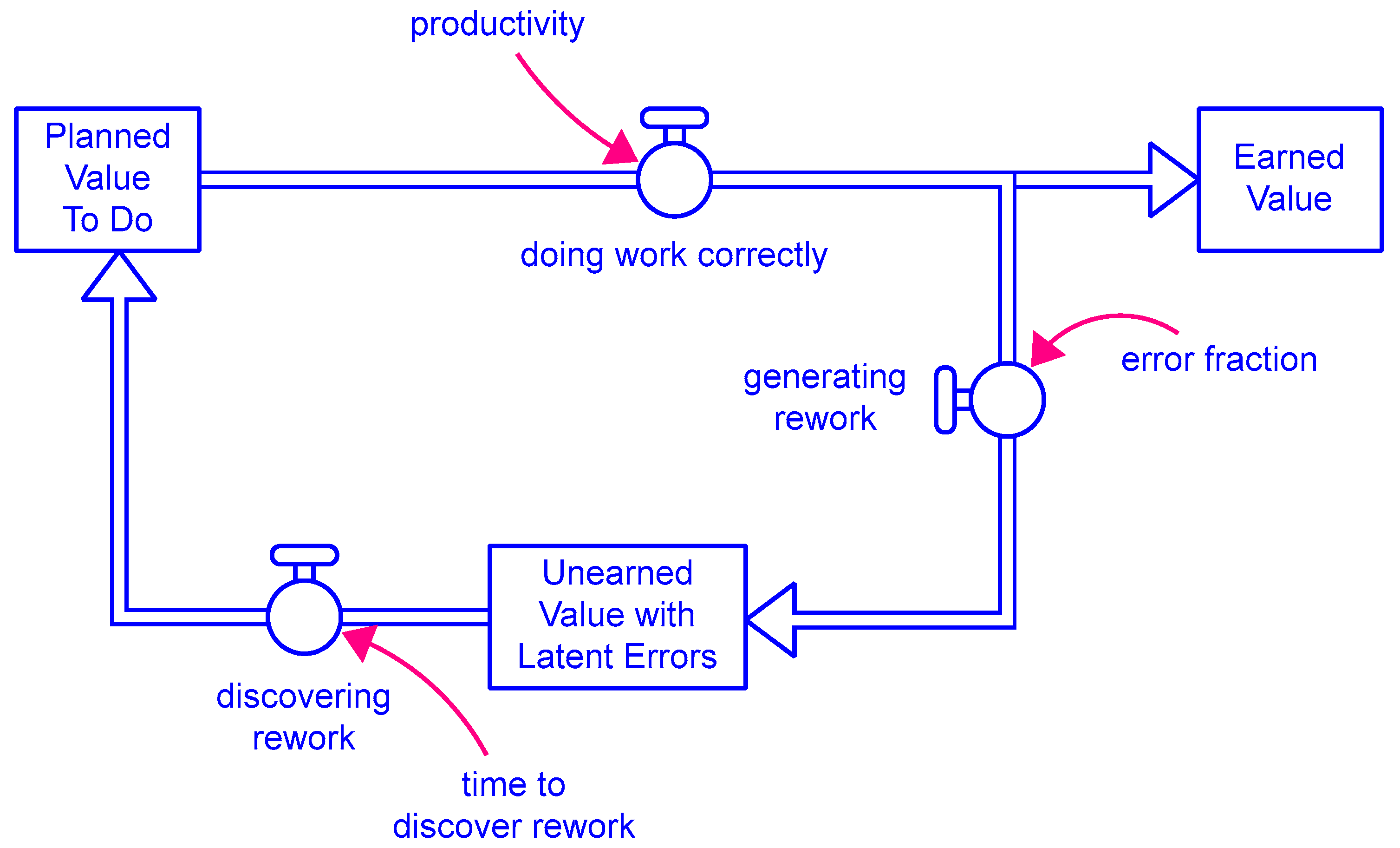
1.4. Projects in Unhealthy Environments with Latent Errors and Required Rework

Latent errors requiring rework and the delayed-discovery rework loop have been at the heart of the dynamics of most models of project work behavior since Pugh Roberts Associates, Cooper, and others first discussed them in 1980 [3]. In Cooper’s work in the 1990s [4,5,22], the Lyneis and Ford models [11,12], and the Chichakly model [10], a major source of delay and cost overruns has been the latent errors that remain undiscovered for a significant part of the project life cycle and then require late-in-the-project correction. “The canonical structure of system dynamics project models is the rework cycle,” [11] (p. 159).

“The rework cycle is, in our opinion, the most important single feature of system dynamics project models. The rework cycle’s recursive nature in which rework generates more rework that generates more rework, etc., creates problematic behaviors that often stretch out over most of a project’s duration and are the source of many project management challenges. PRA developed the first rework cycle model.” [11] (p. 160).

The rework cycle is described here using modern project management language (see Figure 1):

“In this form, the rework cycle includes three pools of work. At the start of a project or project stage, all work resides in the pool Planned Value to Do. Progress is made by applying effort. A fraction of the work being done at any point in time contains errors. Work done correctly enters the Earned Value pool and never needs rework (unless later changes render that work obsolete). However, work containing latent errors enters the Unearned Value with Latent Errors pool. These latent errors are not immediately recognized but are detected as a result of doing downstream work or testing. This discovering of Unearned Value with Latent Errors may occur months or even years after the rework was created. Once discovered, the unearned value is subtracted from the Unearned Value with Latent Errors and added back into the Planned Value to Do pool. The extra Planned Value to Do demands the application of additional effort. Reworking an item can generate or reveal more rework that must be done. Therefore, some reworked items flow through the rework cycle one or more subsequent times” (after [11]) (p. 160).

1.5. Unhealthy Environments with Schedule Pressure

One of the immediate signs of an unhealthy project environment is an unhealthy schedule pressure that forces a project to abandon carefully planned behavior in favor of risky shortcuts that put the whole project at risk. Truly unhealthy schedule pressure appears to have its roots in basic human behavior: “To exert schedule pressure on those around us is a natural, and nearly universal, managerial response to lagging progress. A little bit is good, sharpening the senses and increasing productivity. But like unsolicited criticism, a little goes a long way” [5] (p. 11).

Schedule pressure can be corrosive when it is overapplied. Some executives describe the pressure they place on projects and project managers: “We micro-manage… [and] induce the fear of retribution and we create a … relationship through intimidation …that threatens the project manager with loss of his or her job” [5] (p. 11).

Cooper reports that he has “analyzed dozens of difficult projects, and a case where one or both of these conditions is not present is the exception. The rare exception.” [5] (p. 11).

In the unhealthy project’s dynamics, unhealthy schedule pressure has two immediate consequences: one good and one very bad. Increased schedule pressure does, in fact, increase the day-to-day staff productivity.

Unfortunately, unhealthy schedule pressure also increases the rate of latent errors by a similar small amount [5,10]. These errors, by definition, will require later, remedial work when they are discovered. The undetected latent errors can cause secondary errors in other completed work that further increases the remedial work. Because of the compounding effect of these errors, schedule pressure hurts the project more than it helps the project.

1.6. Real Projects with Schedule Pressure, Latent Errors, and Rework

Lyneis and Ford [11] report that with adjustments to the basic parameters, over 200 projects have fit into this rework cycle structure. The models focused on the undiscovered errors in Unearned Value with Latent Errors and the rework cycle. Many of the projects being modeled were research or design projects with a high degree of uncertainty in the details of the planned exploratory work [4,5]. Additionally, many projects were from a consulting practice that focused on distressed projects in unhealthy environments.

2. Methods

A system dynamics model [23] was built from the rework cycle. This model [10] was modified to use earned value terms, rather than the traditional system dynamics terms, as shown in

Table 1. Traditional names and earned-value names for model variables. The four most important are in bold type. The term “visible” is a new earned-value term made necessary because undiscovered latent errors create an initially hidden, unearned value.

Traditional Name	Earned Value Name
Initial work to do	Planned value (driven by a staffing histogram)
Work to do	Planned value to do
Work done	Earned value
Undiscovered rework	Unearned value with latent errors
Work believed to be done (sum of the above two)	Visible earned value (sum of the above two)
Cumulative person-months	Actual costs
Effective productivity	Visible CPI (cost performance index)

. In addition, a variable with the planned size of the staff each month, that is, the staffing histogram for the project, was added. Later, the planned value of the staff-months (to date) can be compared to the earned value (to date) of completed work. This comparison will allow the dynamic model to get the project back on track. The causal loop diagram (CLD) for this model is shown in Figure 2. This model will be referred to as the Version 1 model. All project costs are measured in staff-months and all projects are initialized with 100 tasks that, in a perfect world, would be completed in 100 staff-months.

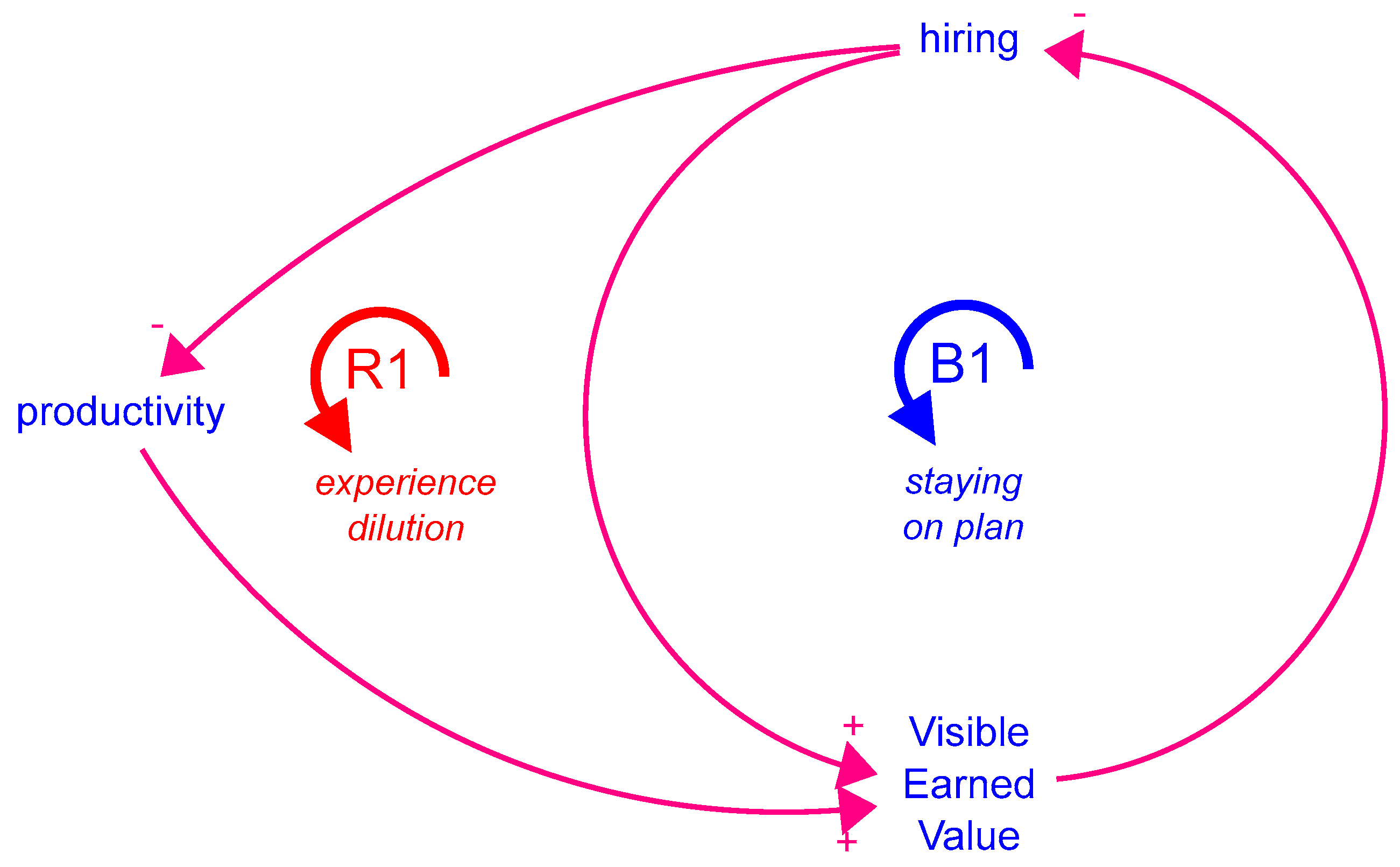
2.1. Structure of the Version 1 Model

The project can respond to needed Visible Earned Value by directly adjusting hiring. If the project falls behind plan, Visible Earned Value goes down (relative to original plan) and hiring in the Model goes up. Increased hiring increases the Visible Earned Value (loop B1: staying on plan). Increased hiring also decreases potential start-up labor productivity because of the experience dilution. Decreased potential labor productivity decreases the Visible Earned Value (relative to original plan) (loop R1: experience dilution). Because the hiring gain is stronger than the productivity loss, the model successfully recovers the project plan and ends on time.

Experience dilution arises as new hires come up to speed on the details of the project and move from being partially effective rookies to 100% effective professionals. The up-to-speed learning requires time and lowers the initial productivity of the staff.

Experience dilution also creates a “desert of resources” at the end of the project. The desert is a period within which any newly hired staff will consume more project time getting up to speed than they will contribute with their efforts, so the desert is a time when the staff can only remain level or decrease. Nevison [24] calculated the desert of resources as a consequence of experience dilution. The desert of resources is also part of the famous, but informal, Brooks’ Law, “Adding staff to a late project only makes it later” [5,25].

The Version 1 model is designed for consistent projects, i.e., projects that are very likely to follow their plan. An initial healthy project begins with a solid plan that includes: a scope statement, a work breakdown structure (WBS), three-point estimates of each activity’s effort and duration, a precedence diagram with a critical path, a risk plan, a scope-change process (a critical element), and a resource histogram with a planned-value-to-date curve (also known as a project performance baseline) [17]. Our mainstream project model has 100 staff-months of cost, a schedule of 24 months, and a resource histogram for how the 100 staff-months of work are deployed over the 24 months.

The model’s plan in Figure 3 begins with a resource histogram showing how the 100 staff-months of work are planned over 24 months, and the planned value (to date) curve showing how they will add up. The histogram has a dramatic peak in the middle.

2.2. Structure of the Version 2 Model

While the Version 1 model should survive the lowered productivity of the staff getting up to speed, the next challenge is unplanned-for work. Unplanned-for work can come from an inconsistent plan, from more difficult than anticipated work, from a less skilled staff, or from a combination of these factors.

An inconsistent plan is often the consequence of deep, unhealthy human biases that err on the side of optimism and professional overconfidence [19]. These biased underestimates of the planned work often bump into the reality of necessary, but unplanned, work that must be done to complete an activity’s deliverable. We will call this necessary-but-unplanned work “unplanned-for work”. For simplicity’s sake, we will assume that the unplanned-for work in the model is the result of recognized work errors that are corrected before being credited to the project.

As this unplanned-for work is being discovered and reported at progress reporting sessions, there may remain additional latent errors, i.e., undetected flaws in the approved work that will require later, additional rework. These efforts will be discussed later in the Version 3 model. The discovery of unhealthy unplanned-for work in real projects suggests the addition of a parameter for this unanticipated work: the percentage unplanned work. This parameter allows the model to account for work that failed to be included in the original plan [1].

Figure 4 shows the Version 2 model’s causal loops. The diagram adds the percentage unplanned work. When a percentage unplanned work appears, the potential productivity goes down and Visible Earned Value goes down (relative to original plan). Then hiring (whose calculation depends on pressure from the Visible Earned Value) increases to eventually recover the plan.

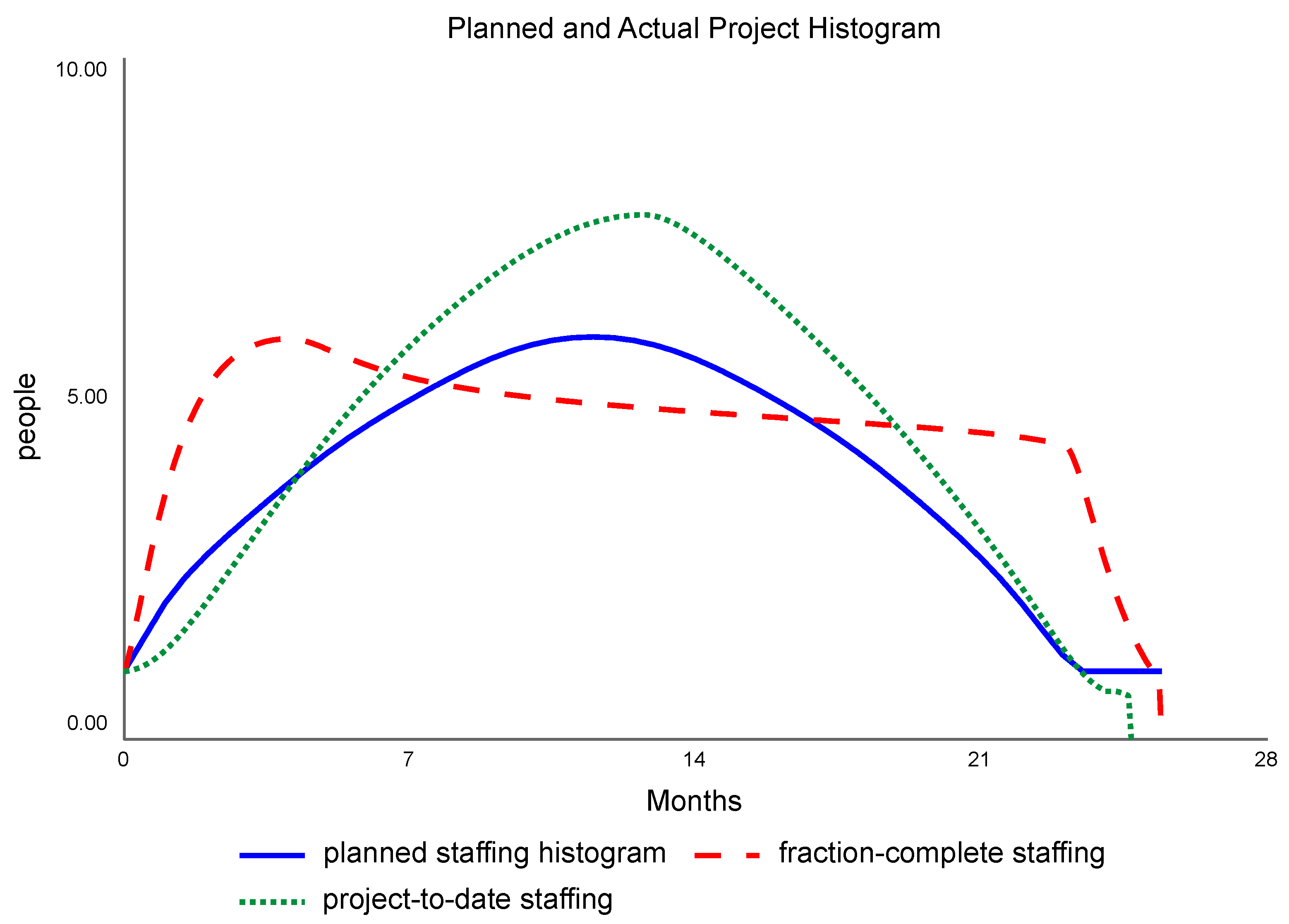
2.3. How This Model Calculates Staffing Needs

Some system dynamics project models have depended on the summary values of the project due date and the project total cost, to calculate the fraction complete and any staffing changes required to complete the project on time. Our model uses an additional healthy detail from the plan: the plan’s resource histogram with its project-to-date variables of Planned Value, Visible Earned Value, and Actual Cost. Without these project-to-date variables, the project is limited to using the summary, fraction-complete method of calculating the needed staffing. Figure 5 compares the two methods:

• The fraction-complete method (Figure 5, dashed red line) adds its 18 staff-months of staffing throughout the project, as it falls behind or gets ahead, because it is completely uninformed by the details of the plan’s staffing histogram. After wildly overstaffing the planned project at the beginning, the method assumes it can understaff the project for 9 months, then work extra at the end to finish on time.
• The project-to-date method (Figure 5, dotted green line), by contrast, adds its 18 staff-months while preserving the shape of the planned staffing histogram.

Rather than the fraction-complete method, our model used the project-to-date method in an effort to remain true to the original planned work intensity as portrayed in the staffing histogram.

2.4. The Structure of the Version 3 Model

Unhealthy projects are subjected to schedule pressure, latent errors, and rework. Figure 6 shows the Version 3 model’s causal loops with unhealthy schedule pressure included (model equations appear in Appendix A). The diagram includes experience dilution, which leads to the experience dilution shown in loops R1 and R1A, and the Unearned Value with Latent Errors loop, which compounds errors (loop R3). This model combines Earned Value and Unearned Value with Latent Errors to create the Visible Earned Value.

If the project Visible Earned Value falls behind schedule, schedule pressure goes up. Schedule pressure is a double-edged sword. It increases potential, planned-work productivity (loop B2A), and it also increases the latent error fraction (loop R2). However, because of the reinforcing errors-on-errors feedback (loop R3 in Figure 6), the detrimental effect of the increased latent error fraction is almost always much larger than the gain in productivity.

The increased latent error fraction increases the Unearned Value with Latent Errors, and, as the errors are discovered, decreases the Visible Earned Value (relative to original plan). That, in turn, increases hiring to recover the plan. Latent errors can cause significant cost increases and schedule delays.

The unhealthy schedule pressure drops the CPI significantly from 0.86 to 0.61. Because the undetected latent errors lurk within the Unearned Value with Latent Errors that is part of the Visible Earned Value, the Visible Earned Value incorrectly overstates the project’s day-to-day progress measurements.

3. Results and Discussion

3.1. Version 1 Model Results

We first explored experience dilution by beginning with one professional on staff, using the initial mainstream parameters for experience dilution, to see if: (i) the project can be completed in 24 months, (ii) the total cost will be close to 100 staff-months, and (iii) the actual staffing pattern can approximate the pattern of the plan’s staffing histogram.

To examine the costs of staffing up, we tested the model with a staff build-up rather than assuming that the staff is already on board. Staffing up also provides a good test of the Version 1 parameters. If the entry activities go smoothly, we may assume Version 1 could follow other projects’ dramatic staffing histograms.

The initial values for some of the model’s main parameters come from the questionnaire responses of 27 white-collar project managers [26]:

• average time to hire = 2 months;
• up-to-speed time (new staff) = 1 month;
• relative productivity of new staff = 60%;
• time to get off the project = 0.5 month.

Figure 7a shows how the model monitored project progress with the two project-to-date, earned-value metrics of Visible Earned Value (solid blue) and Actual Costs (dashed red). Project work accumulated as Visible Earned Value and Actual Costs increased over the 24 months.

Even with the delays in finding new hires and getting people up-to-speed, the project can be completed in 24 months. In addition, the total actual costs for the experience dilution expanded the original plan’s cost from 100 to 103.6 staff-months, and reduced the Visible CPI (cost performance index, aka productivity) from 1.0 to 0.96.

Figure 7b shows that the actual staffing initially fell a little behind, due to entry learning delays, but made it up a little later. In the end, this project used staff roughly when the staff was planned to be used. Even with experience dilution, Version 1’s behavior generally tracks the shape of the planned staffing histogram.

3.2. Version 2 Model’s Results in a Slightly Unhealthy Environment

We next turned to the Version 2 model to test the effect of including additional unplanned work equal to 10% of the planned activity. Figure 8 shows that the model’s Visible CPI dropped at the beginning of the project and then stabilized to conclude at 0.86. This project overran by 18 staff-months of work. The Version 2 model does not yet include the rework cycle, so the new hires do not affect the error rate. As projects operate in less and less healthy environments, we can expect to see even greater cost overruns.

3.3. Version 3 Model’s Results in an Unhealthy Enviroment

What should the project look like in the unhealthy real world? We began with 18 staff-months of unplanned-for work, which reflect the 0.86 Visible CPI we saw with the Version 2 model. For the models surveyed by Chichakly and Lyneis and Ford [10,11], the reported average amount of rework over the whole project was about 40%, while Cooper [5] suggested a typical design project will have about 50% of its effort be rework. These values suggest setting the model’s normal latent error rate to 17%, as this leads to 155 staff-months of work. The 55 additional staff-months could include 18 unplanned staff-months and 37 rework staff-months.

The Version 3 model project simulation in Figure 9a shows a cost of 155 staff-months, including the 55 staff-month overrun. It finished after 28.2 months, a little over four months late. This project also had a Visible CPI of only 0.64 (dotted green).

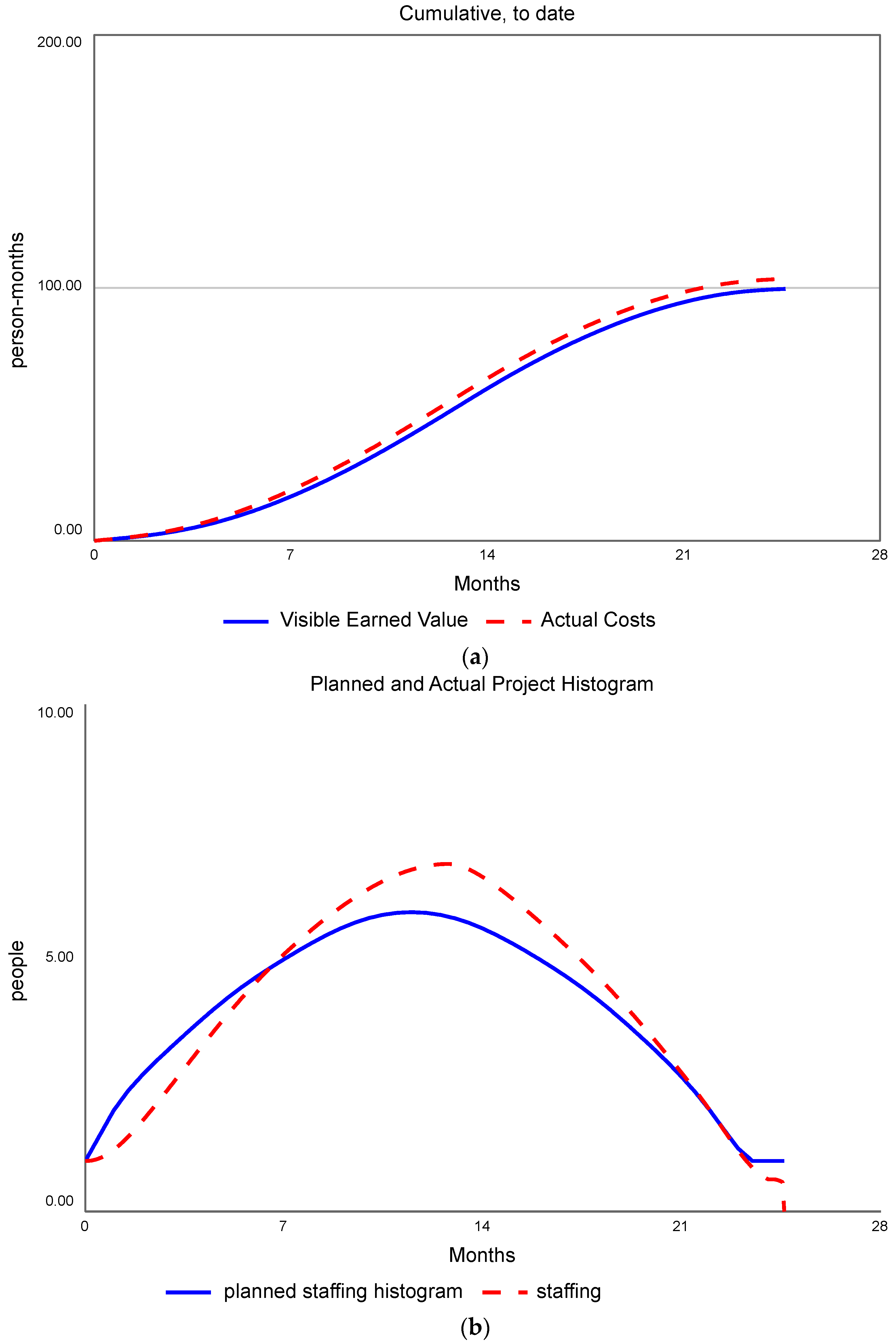
3.4. Earned Value Becomes Visible

Because the Visible Earned Value contains the as-yet-undiscovered Unearned Value with Latent Errors, it overstates the true earned value. The project manager is therefore working with an overly optimistic (higher) Visible Earned Value.

As shown in Figure 9a, The Visible Earned Value was most in error in the middle of the project. However, late in the project, as erroneous work was discovered and corrected, the Visible Earned Value converged to the true earned value. The good news about Visible Earned Value is that it is visible and converges to the true earned value; the bad news is that in the middle of the project, it contains Unearned Value with Latent Errors and overstates the project’s progress to date (compare the solid dark blue and dash-dot orange lines in Figure 9a).

Visible Earned Value makes other indices that depend on earned value overly optimistic in the middle of the project. These include CPI, SPI, and estimate at completion schedule (EAC Sched).

Managing with Visible Earned Value (and all the dependent indices) grows more accurate as errors are discovered and corrected. Visible Earned Value connects the model’s project dynamics to the broad world of modern project-to-date project management.

In Figure 9b, the model exhibited a signature pattern that matches the late swelling in the resource histogram for troubled, unhealthy project environments (see, e.g., [4,5,11,12,27]).

3.5. Version 3 Model’s Results in an Extremely Unhealthy Enviroment

Version 3 shows how the model works in a commonly occurring toxic environment or in extremely unhealthy environments. The literature is full of examples where the original resource histogram peak is not just equaled, but superseded by a subsequent peak brought about by a high rate of latent errors. If we look at a list of common problems cited by over two hundred project managers [22,28], a model where the normal latent error rate might be 25% or more becomes plausible. These problems include: senior management failed to establish a clear goal, scope creep was not controlled, failure to adequately plan (including not enough staff, inadequately skilled staff, unrealistic schedule, insufficient budget), interdepartmental conflicts continuing during the project, communications breakdowns, and poor technical performance by staff. This list, combined with our earlier descriptions of forces that place unhealthy schedule pressure on the project, should make it easy for us to imagine a model where the normal latent error rate is 25%.

In Figure 10a, when the Version 3 model was run with 18 staff-months of unplanned-for work and a normal latent error rate at 25%, the Earned Value (dash-dot orange) became widely separated from the Visible Earned Value (solid dark blue). The total project costs expanded to 190 staff-months with a Visible CPI of 0.52 (dotted green) and delivery date that slipped 7 months (to 31 months). In Figure 10b, the model exhibited a signature pattern that matches the late second peak in the resource histograms for troubled, extremely unhealthy, project environments (see, e.g., [4,5,11,12,27]).

3.6. Version 3 Model’s Scope Management

In addition to preserving the schedule by increasing staff, the Version 3 model can preserve the schedule by reducing scope. In general, the scope is reduced when a project is equally staffed and no additional costs can be added to the project. When limited to a constant level of staffing, reducing the scope can allow a project to finish on schedule. (See Figure 11b for this project’s level staffing at 4.17 staff).

The model’s structure also allows the project to increase its scope to accommodate customer requests that have been approved by the project team. By definition, any change in scope in the model is an approved change to the current plan for the project (a healthy, standard practice for maintaining an approved project baseline). An unhealthy project environment could be one in which unapproved changes have been allowed into the project, or one where a process for scope change management has not been defined or enforced.

The Version 3 model can also show the effects of scope creep (increased scope) over any portion of the entire project (see [24] for an example). A convenient way to think about the model’s current scope goal is that it is the current planned value target for the whole project, the target total of all the staff-months of the project’s deliverables, also known as the “currently approved budget.”

Figure 11a shows how 18 staff-months of unplanned work and a 17% normal latent error rate led the project to respond with a final Current Scope Goal of 69 staff-months. The project’s final values include a Visible Earned Value of 69 and Current Scope Goal of 69 staff-months (a 31% scope reduction). The final Actual Costs were 97 staff-months in 24 months.

4. Conclusions

The project experiments began with a simple project and a simple project model. Through successive versions, the model was expanded and the project environment became more hostile.

Table 2. The evolutionary project’s versions.

Model’s Version	Used to Illustrate…
Version 1	3.6 staff-months of experience dilution
Version 2	18 staff-months of extra work from unplanned-work
Version 3	55 and 90 staff-months of extra work—18 unplanned-for and the rest from latent error rework
Variation of Version 3	Constant staffing, extra work forcing a 31 staff-month scope reduction to maintain schedule and cost

shows how as the environment grew more and more hostile, successive versions of the model, with the help of earned value, managed the project.

This project model weaves together ideas from earned value project management and systems dynamics. From earned value, it includes the planned staffing histogram and the project performance baseline, reveals the unplanned-for-effort in the typical Cost Performance Index behavior, and uses the actual cost to date and the earned value to date to assess progress on the project.

Using system dynamics, the model captures the delay and cost of experience dilution, the effects of schedule pressure, and the vicious cycle effects of latent errors in the rework cycle. The model tracks latent undiscovered errors in the renamed variables of Visible Earned Value and Unearned Value With Latent Errors. It adjusts project staffing, scope, or both to complete the project on schedule.

A new method of estimating the remaining work, and therefore the staff required to meet the schedule, called project-to-date, was proposed in place of the commonly used fraction-complete method. The staffing histogram generated by this method stays much closer to plan than when using fraction complete.

We set out to show that by integrating earned value concepts into the traditional system dynamic project model based on the rework cycle, that model can reproduce observed real-world behaviors in successively more unhealthy projects, and can be used to correct a project that is not meeting its plan. In particular, starting with a 100-task project with a plan to be completed in 24 months, the Version 3 model, under difficult circumstances, is able to complete the project in 31 months. When told the schedule is more important than scope, the model successfully decreased the scope of the project to meet the schedule.

This model, with its combination of concepts from earned value project management and system dynamics, demonstrates that a dynamic model of a traditional project can adjust to increasingly unhealthy actual project behaviors in ways that preserve the signature pattern of staffing histograms observed in the real world. It also gives managers a tool that can help bring unhealthy projects back on schedule.

References

1. Roberts, E.B. The Dynamics of Research and Development; Harper and Row: New York, NY, USA, 1964. [Google Scholar]
2. Roberts, E.B. A Simple Model of R&D Project Dynamics. R&D Manag. 1974, 5, 1–15. [Google Scholar] [CrossRef]
3. Cooper, K.G. Naval Ship Production: A Claim Settled and a Framework Built. Interfaces 1980, 10, 20–36. [Google Scholar] [CrossRef]
4. Cooper, K.G. The Rework Cycle: Benchmarks for the Project Manager. Proj. Manag. J. 1993, 24, 17–21. [Google Scholar]
5. Cooper, K.G. The $2,000 Hour: How Managers Influence Project Performance through the Rework Cycle. Proj. Manag. J. 1994, 25, 11–24. [Google Scholar]
6. Abdel-Hamid, T.; Madnick, S.E. Software Project Dynamics: An Integrated Approach; Prentice-Hall: Englewood Cliffs, NJ, USA, 1991. [Google Scholar]
7. Chichakly, K.J. The Bifocal Vantage Point: Managing Software Projects from a Systems Thinking Perspective. Am. Program. 1993, 6, 18–25. [Google Scholar]
8. Homer, J.; Sterman, J.; Greenwood, B.; Perkola, M. Delivery Time Reduction in Pulp and Paper Mill Construction Projects: A Dynamic Analysis of Alternatives. In Proceedings of the 1993 International System Dynamics Conference, Cancún, Mexico, 20–22 July 1993. [Google Scholar]
9. Ford, D.N.; Sterman, J.D. Dynamic Modeling of Product Development Processes. Syst. Dynam. Rev. 1998, 14, 31–68. [Google Scholar] [CrossRef]
10. Chichakly, K.J. Modeling Agile Development: When Is It Effective? In Proceedings of the International Conference of the System Dynamics Society, Boston, MA, USA, 29 July–2 August 2007. [Google Scholar]
11. Lyneis, J.M.; Ford, D.N. System Dynamics Applied to Project Management: A Survey, Assessment, and Directions for Future Research. Syst. Dyn. Rev. 2007, 23, 157–189. [Google Scholar] [CrossRef]
12. Ford, D.N.; Lyneis, J.M. System Dynamics Applied to Project Management: A Survey, Assessment, and Directions for Future Research. In System Dynamics; Springer: New York, NY, USA, 2020; pp. 285–314. [Google Scholar] [CrossRef]
13. Akkermans, H.; van Oorschot, K.E. Pilot Error? Managerial Decision Biases as Explanation for Disruptions in Aircraft Development. Proj. Manag. J. 2016, 47, 79–102. [Google Scholar] [CrossRef]
14. Fleming, Q.W.; Koppelman, J.M. Earned Value Project Management, 4th ed.; Project Management Institute: Newtown Square, PA, USA, 2010. [Google Scholar]
15. Christensen, D.; Payne, K. Cost Performance Index Stability: Fact or Fiction? J. Parametr. 1992, 12, 27–40. [Google Scholar] [CrossRef]
16. Christensen, D.S. An Analysis of Cost Overruns on Defense Acquisition Contracts. Proj. Manag. J. 1993, 3, 43–48. [Google Scholar]
17. PMI. The Guide to the Project Management Body of Knowledge (PMBok Guide), 6th ed.; Project Management Institute: Newtown Square, PA, USA, 2017. [Google Scholar]
18. Narbaev, T. Earned Value and Cost Contingency Management: A Framework Model for Risk Adjusted Cost Forecasting. J. Mod. Proj. Manag. 2017, 4, 12–19. [Google Scholar] [CrossRef]
19. Kahneman, D. Thinking Fast and Slow; Farrar, Straus and Giroux: New York, NY, USA, 2011. [Google Scholar]
20. Radice, R.A. High Quality Low Cost Software Inspections; Paradoxicon Publishing: Andover, MA, USA, 2002. [Google Scholar]
21. Shumate, K.; Snyder, T. Software Project Reporting. In Proceedings of the Conference on TRI-Ada ‘94, Baltimore, MD, USA, 6–11 November 1994; pp. 41–45. [Google Scholar] [CrossRef]
22. Cooper, K.G. Power of the People. PM Netw. 1999, 13, 43–47. [Google Scholar]
23. Forrester, J.W. Industrial Dynamics; MIT Press: Cambridge, MA, USA, 1961. [Google Scholar]
24. Nevison, J.M. Working the ‘Educated’ Plan: How Effective Is Corrective Staffing in a Typical White-Collar Project? J. Mod. Proj. Manag. 2015, 2. [Google Scholar] [CrossRef]
25. Brooks, F.P. The Mythical Man-Month, Anniversary ed.; Addison Wesley: Reading, MA, USA, 1995. [Google Scholar]
26. Nevison, J.M. White Collar Project Management Questionnaire Report. Internal Working Paper; New Leaf Project Management: Concord, MA, USA, 1992. [Google Scholar]
27. Cooper, K.G.; Reichelt, K.S. Quantifying Disruption: Rigorous Analysis of a Challenging Problem. In Proceedings of the Project Management Institute Annual Seminars & Symposium, San Antonio, TX, USA, 3–10 October 2002. [Google Scholar]
28. Taylor, J. A Survival Guide for Project Managers; Amacom: New York, NY, USA, 1998. [Google Scholar]
Figure 1. Rework cycle.
Systems 09 00088 g001
Figure 2. Causal loop diagram of the version 1 model.
Systems 09 00088 g002
Figure 3. Planned value to date (dashed red) and resource histogram (dotted green, right).
Systems 09 00088 g003
Figure 4. Causal loop diagram of the Version 2 model.
Systems 09 00088 g004
Figure 5. Scenario with 18 staff-months’ unplanned-for costs, planned (solid blue) against the fraction-complete method (dashed red) and project-to-date method (dotted green).
Systems 09 00088 g005
Figure 6. Causal loop diagram of the Version 3 model.
Systems 09 00088 g006
Figure 7. (a) Version 1 model’s earned value variables. (b) Version 1 model’s planned (solid blue) and actual (dashed red) staff histogram.
Systems 09 00088 g007
Figure 8. Version 2 model run with 118 staff-months of cost. Visible CPI is on the right axis.
Systems 09 00088 g008
Figure 9. (a) Version 3 model run with 18 staff-months’ unplanned-for costs, a normal latent error rate of 17%, and a total amount of unplanned work, latent error rework of 18 + 37 staff-months (55%). (b) Version 3 model run with 18 staff-months’ unplanned-for costs and a normal latent error rate of 17% shows the persistent late staffing in the staff histogram.
Systems 09 00088 g009
Figure 10. (a) Project-to-date method with 18 staff-months’ unplanned-for work and 25% normal latent error rate. (b) Project-to-date method with 18 staff-months’ unplanned-for work and 25% normal latent error rate. Our extremely unhealthy project in a toxic environment exhibits a very high error rate and work pattern that matches the reported behavior of real projects operating in toxic environments.
Systems 09 00088 g010aSystems 09 00088 g010b
Figure 11. (a) Project-to-date methods adjusting scope, beginning with a level staff of 4.17 people, following the plan of a level histogram with 18 staff-months’ unplanned work and a 17% normal latent error rate. (b) The level staffing forces a reduction in scope to meet the schedule.
Systems 09 00088 g011