
Channel Identification Based on Cumulants, Binary Measurements, and Kernels

 , , , ,
  and
and 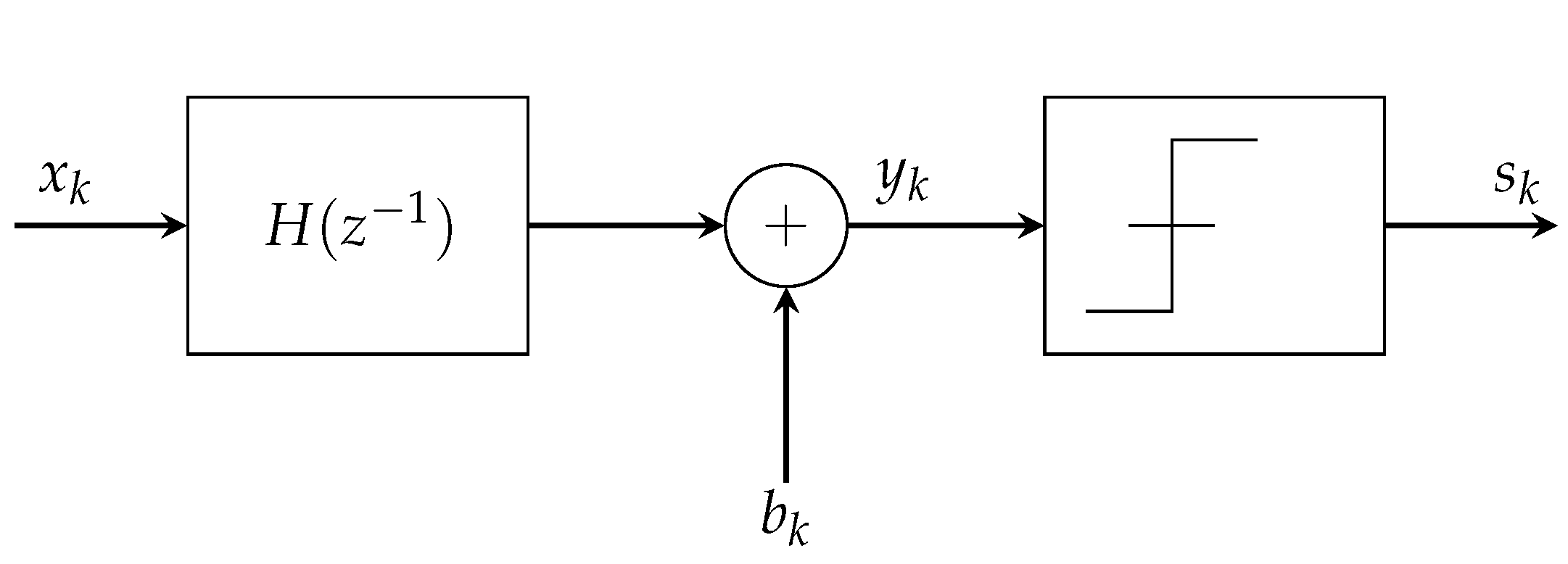
Abstract
1. Introduction
2. Problem Statement
3. Channel Identification Based on Cumulants
3.1. First Algorithm: Alg1
- The parameters for are estimated from the values of using the following solution:withand indicates the absolute value of x.
- The parameters are estimated by:
3.2. Second Algorithm: Alg2
3.3. Third Algorithm: Alg3
4. Binary Output Measurement Algorithms
4.1. LIMBO Method
- A.1: .
- A.2: is a random process such that:
- −
- The probability density function (pdf) of is non-zero on the unit sphere.
- −
- verifies the -mixing condition [47].
- A.3: represents the noise, which is uncorrelated with the input sequence.
4.2. Recursive Least Squares (RLS) Method
- B.1: , where is the norm.
- B.2: At any time k, .
- B.3: The noise sequence is an i.i.d. sequence of random variables with a mean of zero and finite covariance, and it is uncorrelated with the input sequence.
4.3. Method Based on SVM
- C.1: The static gain of the system is known.
- C.2: is such that at any time k, .
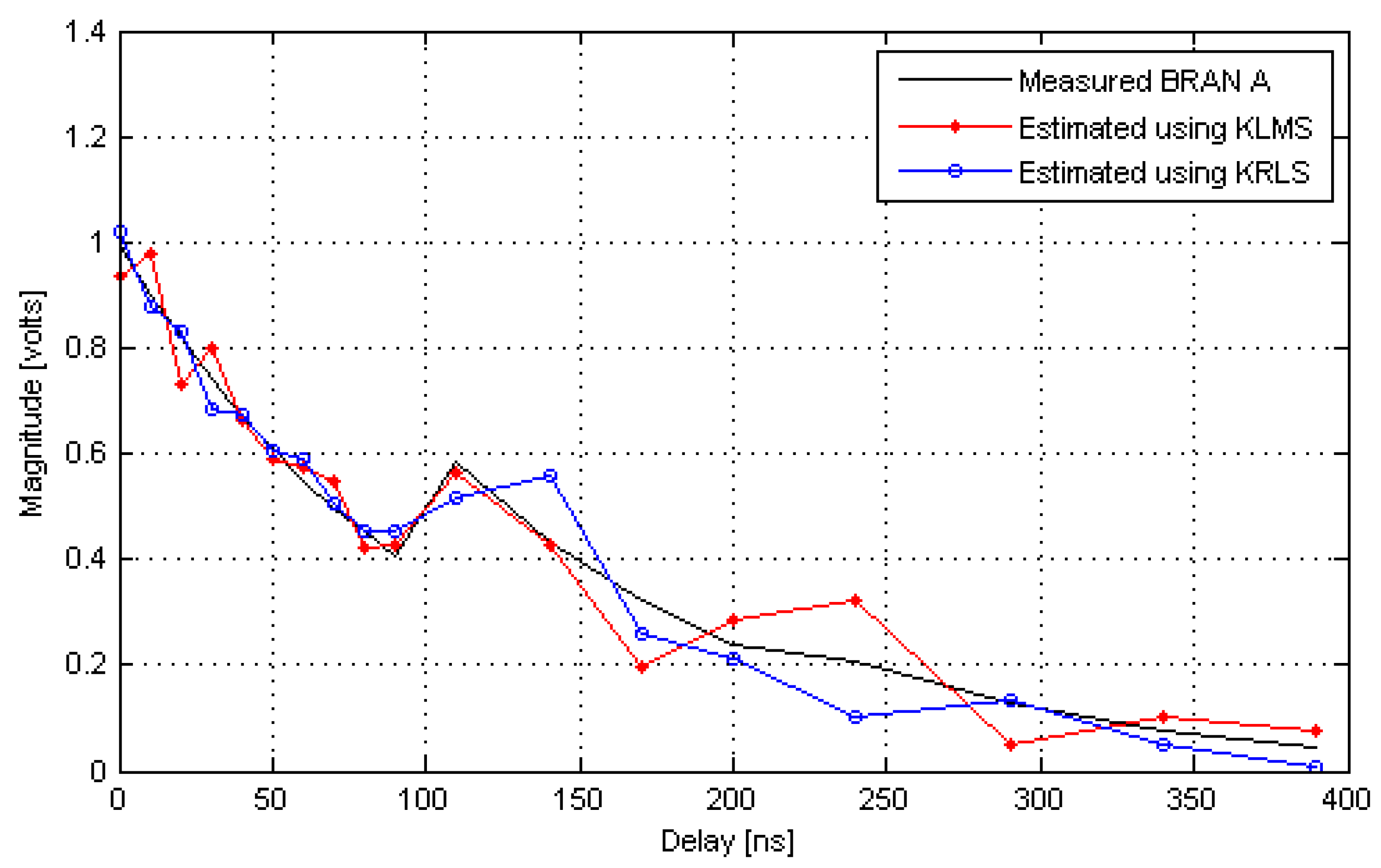
5. Kernel-Based Channel Identification
5.1. Kernel Recursive Least Squares Algorithm
5.2. Kernel Least Mean Square Algorithm
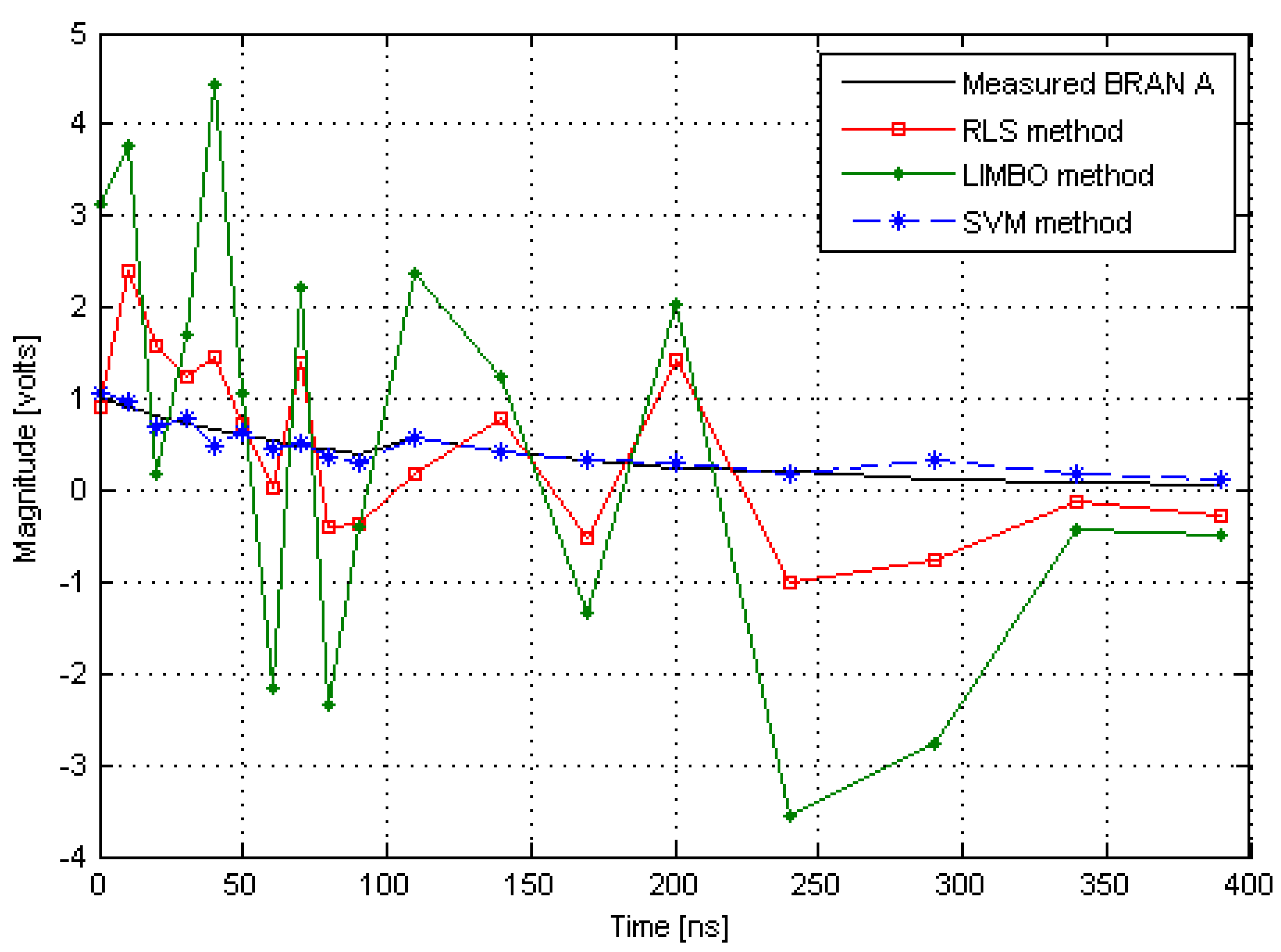
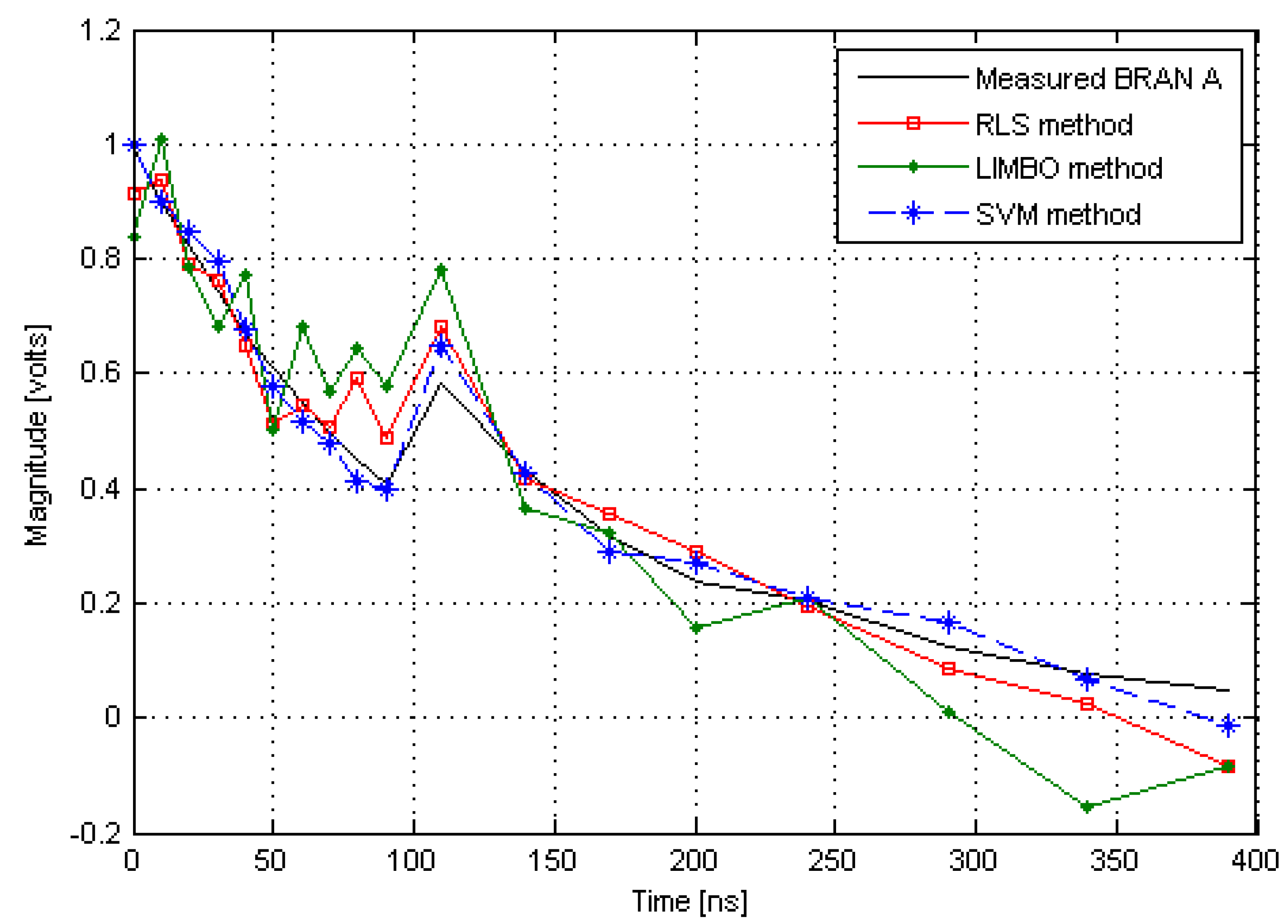
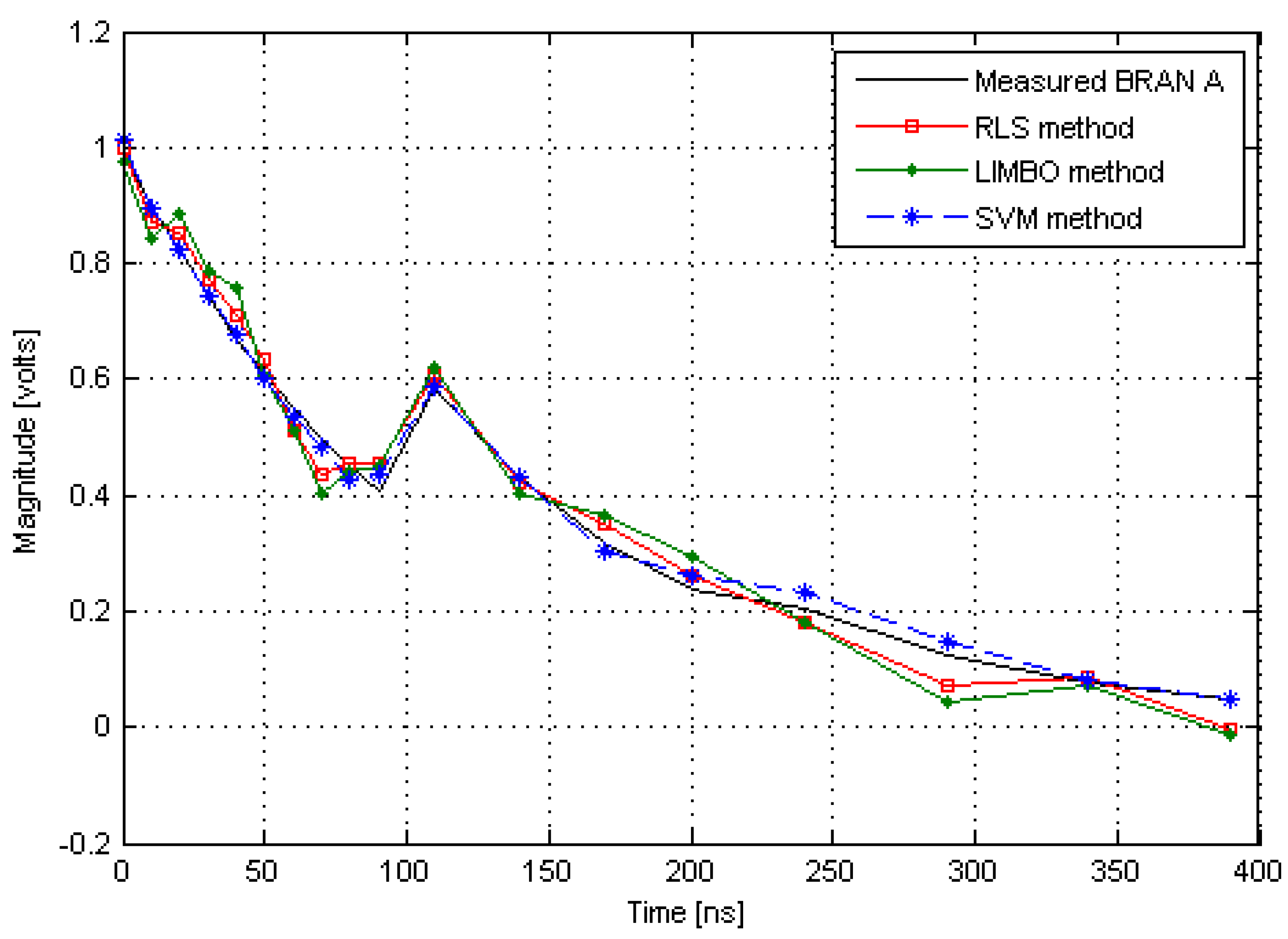
6. Simulation Results
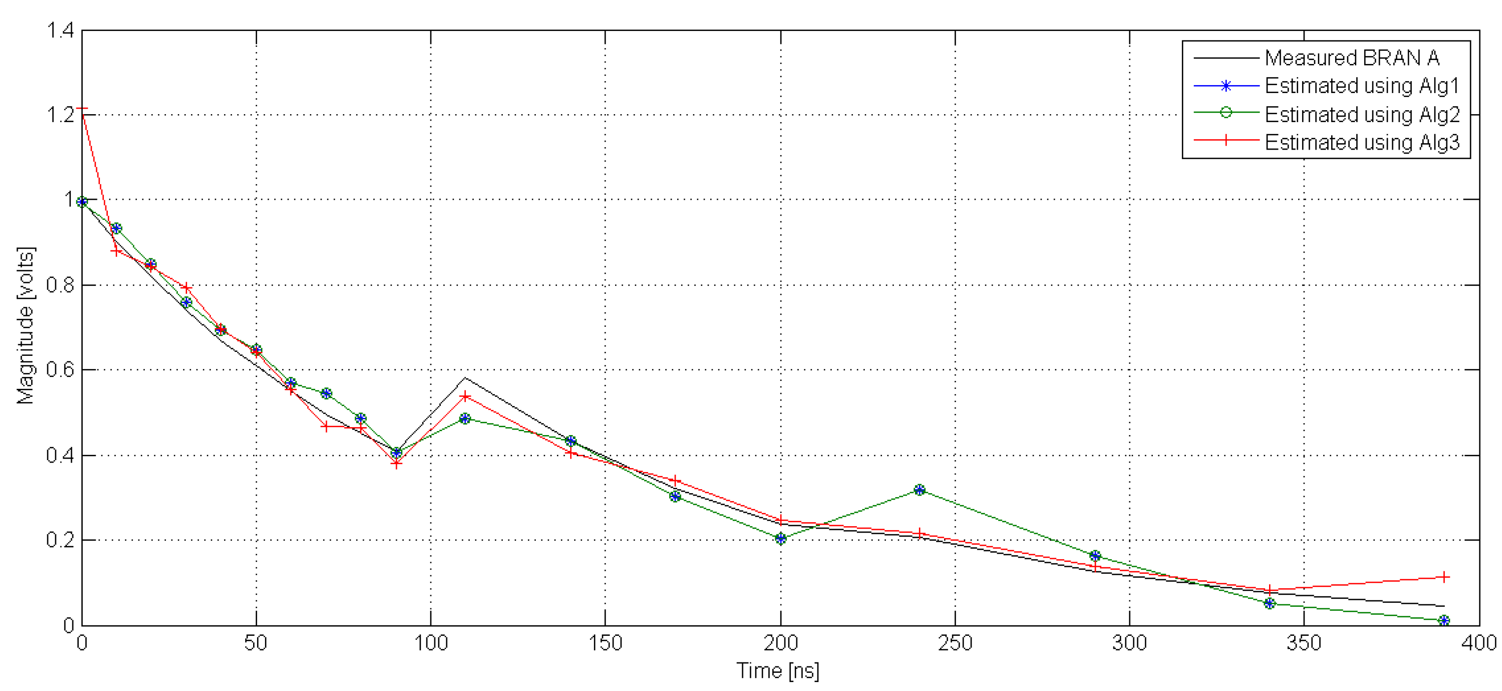
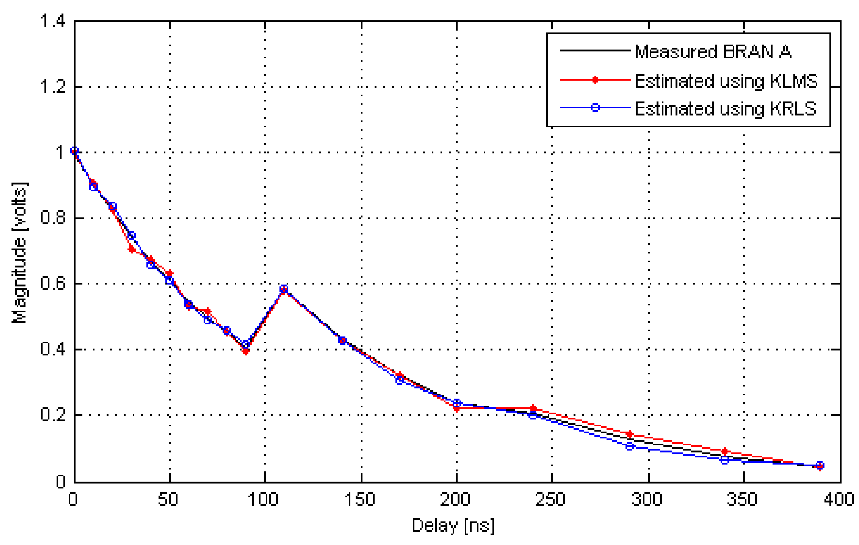
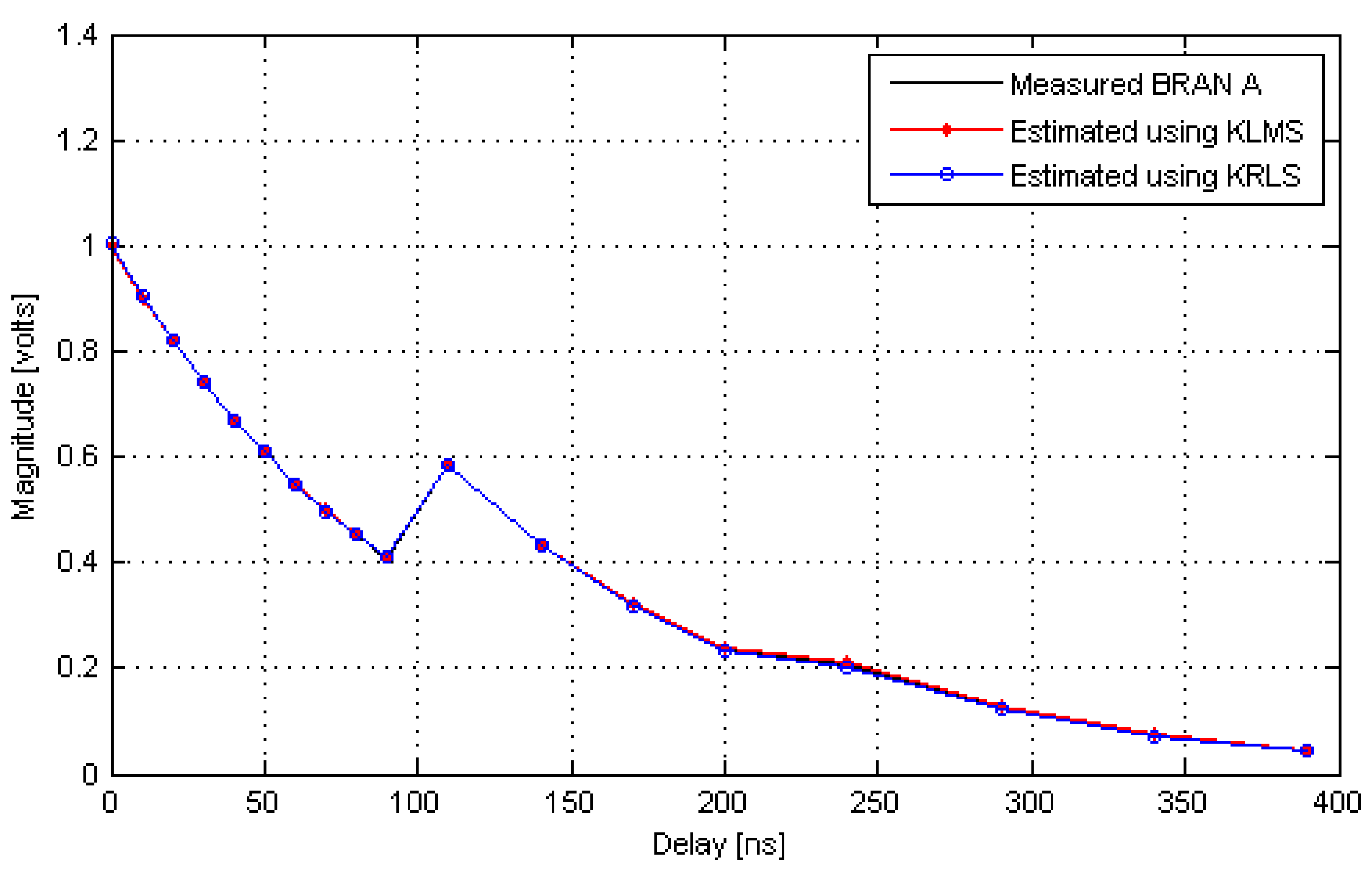
6.1. Impulse Response Parameter Estimation
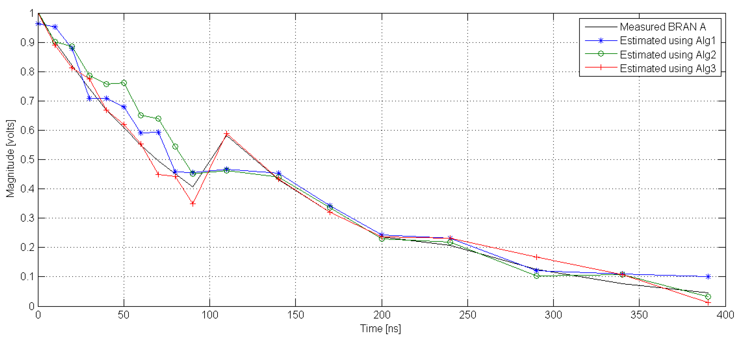
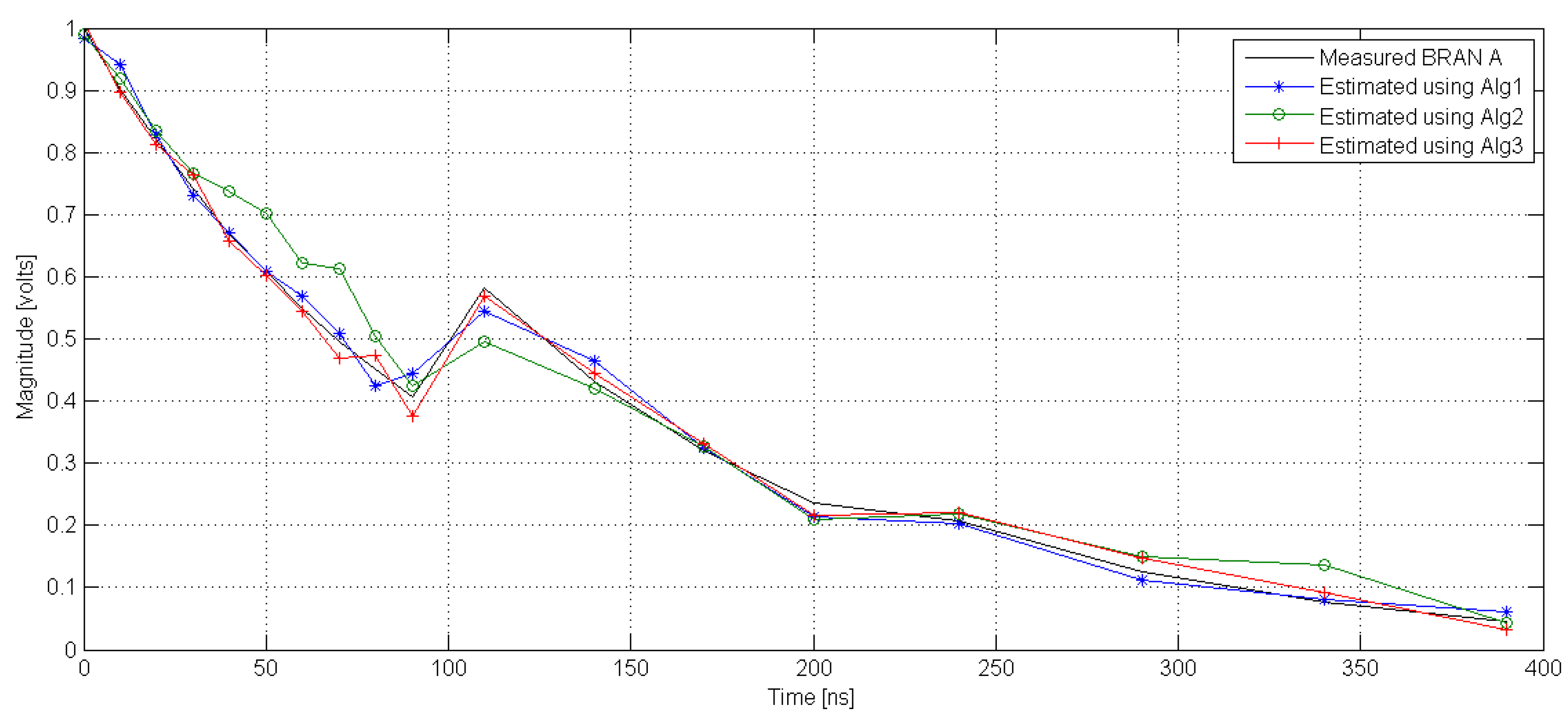
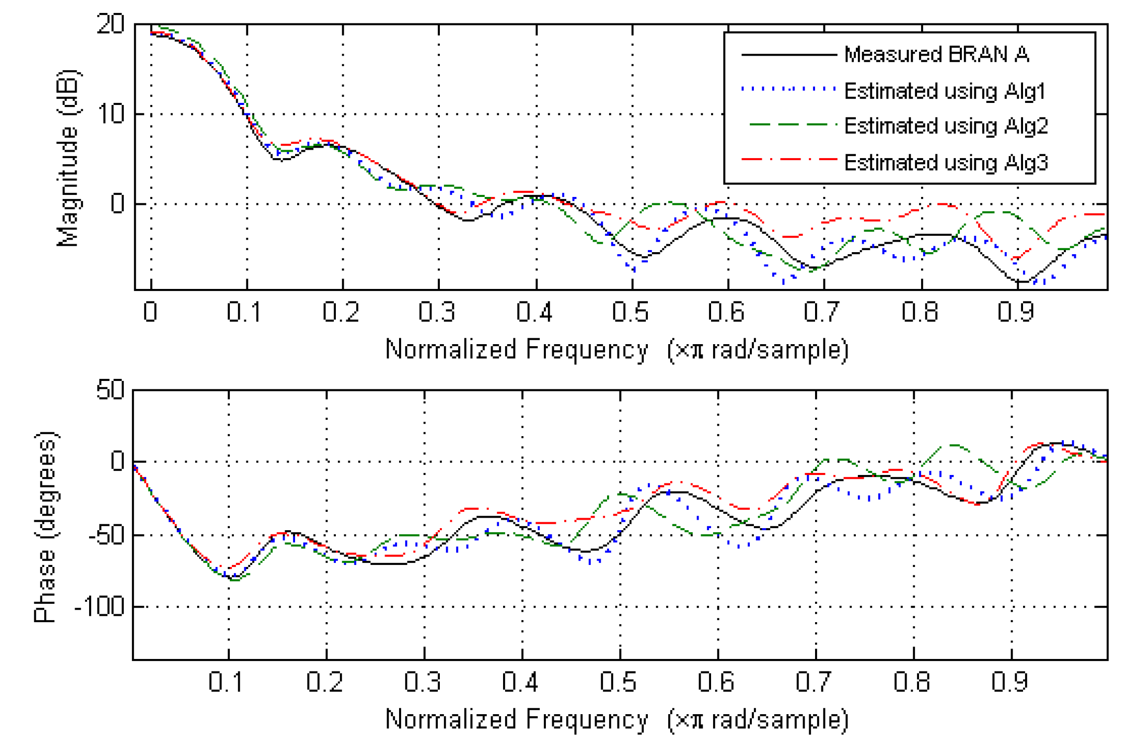
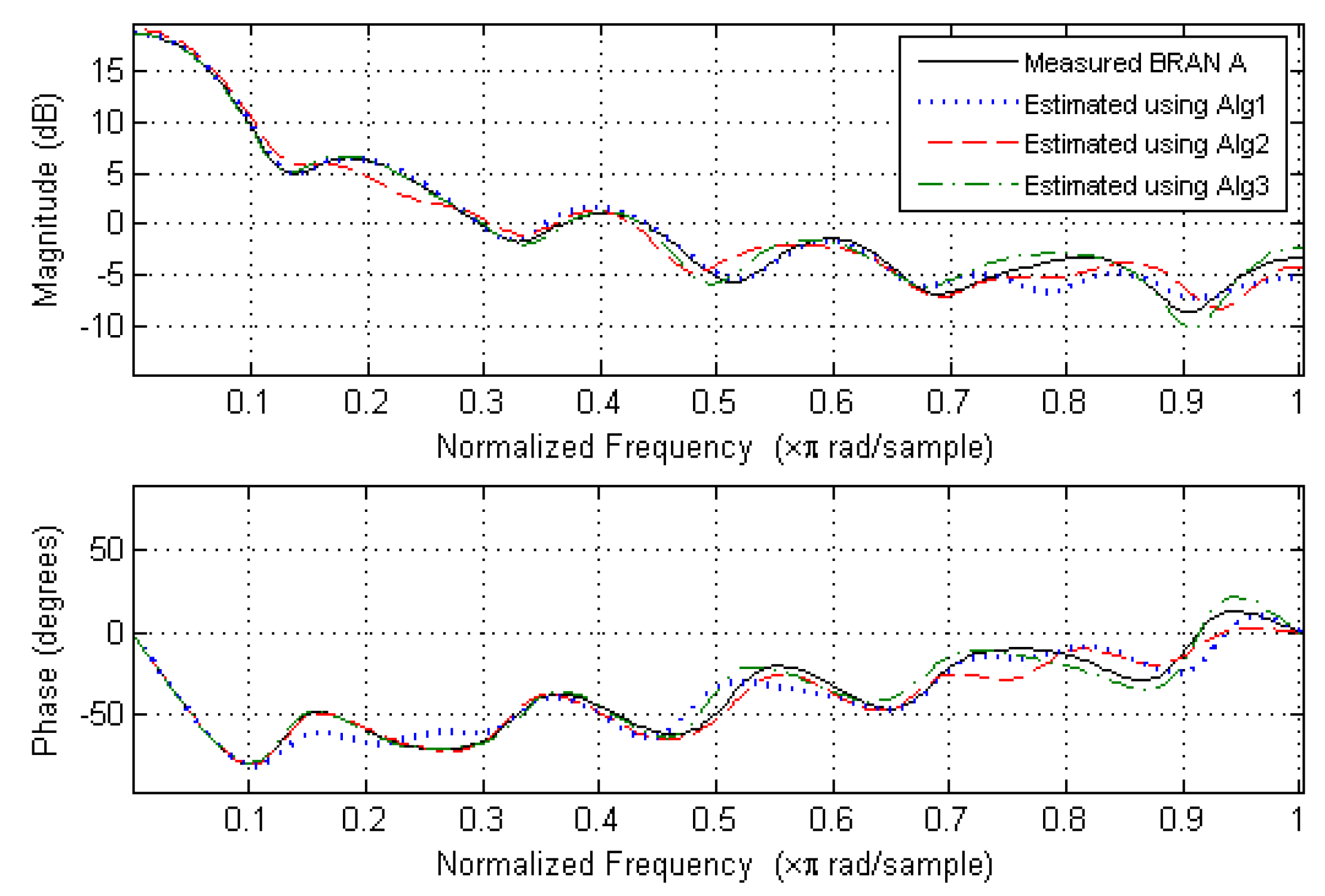
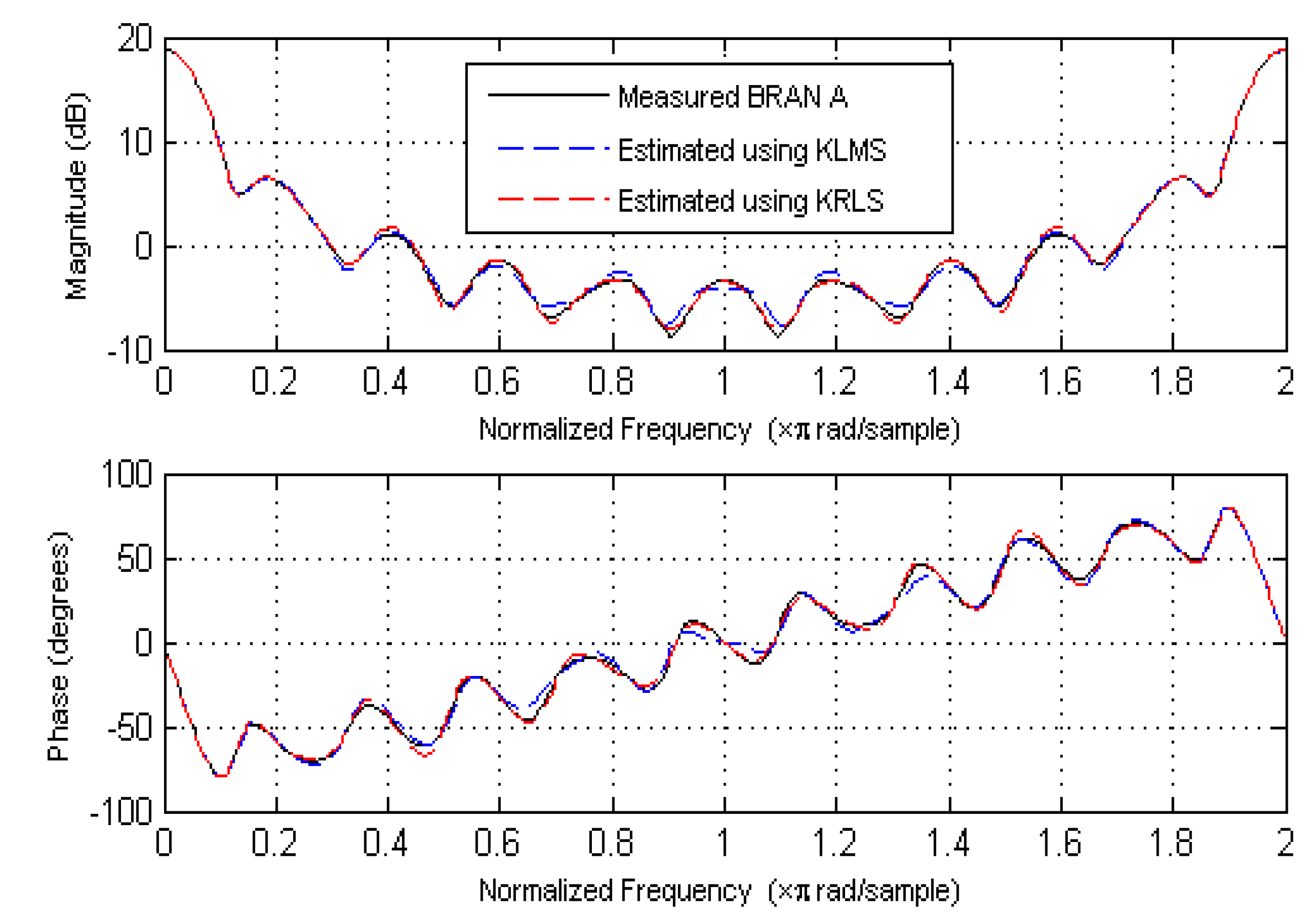
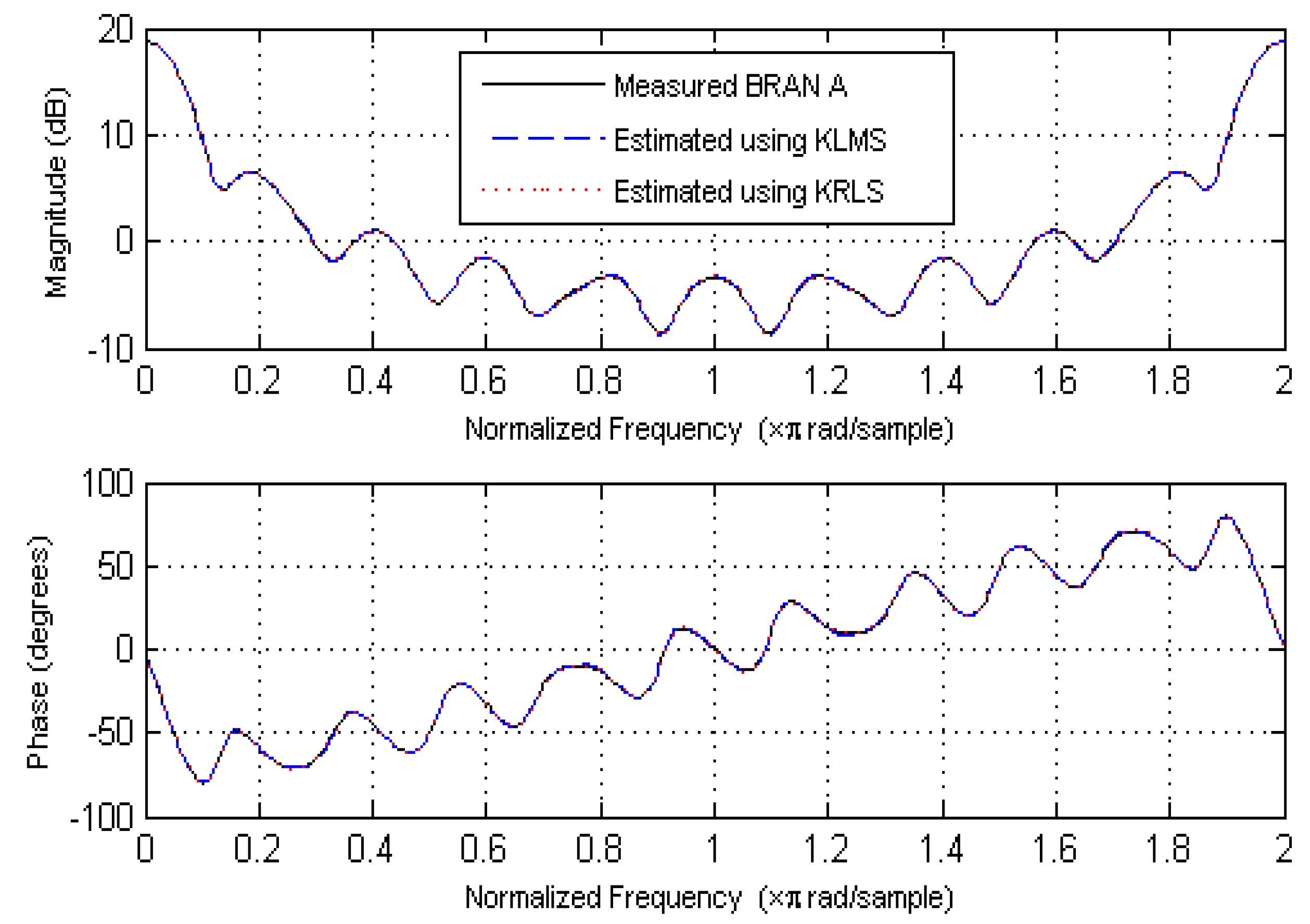
6.2. Magnitude and Phase Estimation
7. Conclusions
Author Contributions
Funding
Conflicts of Interest
References
- Safi, S.; Zeroual, A. MA system identification using higher order cumulants: Application to modelling solar radiation. Int. J. Stat. Comput. Simul. 2002, 72, 533–548. [Google Scholar] [CrossRef]
- Safi, S.; Zeroual, A. Blind parametric identification of non-Gaussian FIR systems using higher order cumulants. Int. J. Syst. Sci. 2004, 35, 855–867. [Google Scholar] [CrossRef]
- Safi, S.; Zeroual, A. Blind non-minimum phase channel identification using 3rd and 4th order cumulants. Int. J. Signal Process. 2008, 4, 158–168. [Google Scholar]
- Sadler, B.M.; Giannakis, G.B.; Lii, K.S. Estimation and detection in non-Gaussian noise using higher order statistics. IEEE Trans. Signal Process. 1994, 42, 2729–2741. [Google Scholar] [CrossRef]
- Wang, J.; He, Z. Criteria and algorithms for blind source separation based on cumulants. Int. J. Electron. 1996, 81, 1–14. [Google Scholar] [CrossRef]
- Yin, G.G.; Zhao, Y.; Zhang, J.F. Identification input design for consistent parameter estimation of linear systems with binary-valued output observations. IEEE Trans. Autom. Control 2008, 53, 867–880. [Google Scholar]
- Zhang, J.F.; Yin, G.G. System identification using binary sensors. IEEE Trans. Autom. Control 2003, 48, 1892–1907. [Google Scholar]
- Godoy, B.I.; Goodwin, G.C.; Agüero, J.C.; Marelli, D.; Wigren, T. On identification of FIR systems having quantized output data. Automatica 2011, 47, 1905–1915. [Google Scholar] [CrossRef]
- Safi, S.; Zeroual, A. Blind identification in noisy environment of nonminimum phase finite impulse response (FIR) system using higher order statistics. Syst. Anal. Model. Simul. 2003, 43, 671–681. [Google Scholar] [CrossRef]
- Antari, J.; Iqdour, R.; Safi, S.; Zeroual, A.; Lyhyaoui, A. Identification of quadratic non linear systems using higher order statistics and fuzzy models. In Proceedings of the IEEE International Conference On Acoustic, Speech and Signal Process (ICASSP), Toulouse, France, 14–19 May 2006; pp. 712–715. [Google Scholar]
- Zidane, M.; Safi, S.; Sabri, M. Extending HOC-based methods for identifying the diagonal parameters of quadratic systems. Signal Image Video Process. 2018, 12, 125–132. [Google Scholar] [CrossRef]
- Zidane, M.; Safi, S.; Sabri, M.; Boumezzough, A. Identification and equalization using higher order cumulants in MC-CDMA systems. In Proceedings of the 2014 5th Workshop on Codes, Cryptography and Communication Systems, WCCCS 2014, El Jadida, Morocco, 27–28 November 2014; pp. 81–85. [Google Scholar]
- Zidane, M.; Safi, S.; Sabri, M.; Boumezzough, A.; Frikel, M. Broadband radio access network channel identification and downlink MC-CDMA equalization. Int. J. Energy Inform. Commun. 2014, 5, 13–34. [Google Scholar] [CrossRef]
- Frikel, M.; Targui, B.; Hamon, F.; M’Saad, M. Adaptive equalization using controlled equal gain combining for uplink/downlink MC-CDMA systems. Int. J. Signal Process. 2008, 4, 230–237. [Google Scholar]
- Zidane, M.; Safi, S.; Sabri, M. Measured and estimated data of non-linear BRAN channels using HOS in 4G wireless communications. Data Brief 2018, 17, 1136–1148. [Google Scholar] [CrossRef]
- Nikias, C.L.; Mendel, J.M. Signal processing with higher-order spectra. IEEE Signal Process. Mag. 1993, 10, 10–37. [Google Scholar] [CrossRef]
- Wang, A.; Li, R. Research on digital signal recognition based on higher order cumulants. In Proceedings of the 2019 International Conference on Intelligent Transportation, Big Data & Smart City (ICITBS), Changsha, China, 12–13 January 2019; pp. 586–588. [Google Scholar]
- Simic, M.; Stankovic, M.; Orlic, V.D. Automatic Modulation Classification of Real Signals in AWGN Channel Based on Sixth-Order Cumulants. Radioengineering 2021, 30, 205. [Google Scholar] [CrossRef]
- Khosraviyani, M.; Kalbkhani, H.; Shayesteh, M.G. Higher order statistics for modulation and STBC recognition in MIMO systems. IET Commun. 2019, 13, 2436–2446. [Google Scholar] [CrossRef]
- Anderson, J.M.; Giannakis, G.B. Noisy input/output system identification using cumulants and the Steiglitz-McBride algorithm. IEEE Trans. Signal Process. 1996, 44, 1021–1024. [Google Scholar] [CrossRef]
- Kaiser, T. MA-model identification using modulated moment sequences. Signal Process. 1995, 47, 85–103. [Google Scholar] [CrossRef]
- Proakis, J.; Salehi, M. Digital Communications, 5th ed.; McGraw-Hill: New York, NY, USA, 2007. [Google Scholar]
- Ju, L.; Zhenya, H. Blind identification and equalization using higher-order cumulants and ICA algorithms. In Proceedings of the International Conference Neural Networks and Brain (ICNN B’98), Beijing, China, 13–15 October 1998. [Google Scholar]
- Zhang, X.D.; Zhang, Y.S. FIR system identification using higher order statistics alone. IEEE Trans. Signal Process. 1994, 42, 2854–2858. [Google Scholar] [CrossRef]
- Guo, J.; Zhao, Y.; Sun, C.Y.; Yu, Y. Recursive identification of FIR systems with binary-valued outputs and communication channels. Automatica 2015, 60, 165–172. [Google Scholar] [CrossRef]
- Guo, J.; Yin, G.; Zhao, Y.; Zhang, J.F. Identification of Wiener systems with quantized inputs and binary-valued output observations. Automatica 2017, 78, 280–286. [Google Scholar] [CrossRef]
- Yin, G.G.; Zhang, J.F. Joint identification of plant rational models and noise distribution functions using binary-valued observations. Automatica 2006, 42, 535–547. [Google Scholar]
- Pouliquen, M.; Menard, T.; Pigeon, E.; Gehan, O.; Goudjil, A. Recursive system identification algorithm using binary measurements. In Proceedings of the 2016 European Control Conference (ECC), Aalborg, Denmark, 29 June–1 July 2016; pp. 1353–1358. [Google Scholar]
- Goudjil, A.; Pouliquen, M.; Pigeon, E.; Gehan, O.; M’Saad, M. Identification of systems using binary sensors via support vector machines. In Proceedings of the 2015 54th IEEE Conference on Decision and Control (CDC), Osaka, Japan, 15–18 December 2015; pp. 3385–3390. [Google Scholar]
- Jafari, K.; Juillard, J.; Roger, M. Convergence analysis of an online approach to parameter estimation problems based on binary observations. Automatica 2012, 48, 2837–2842. [Google Scholar] [CrossRef]
- Guo, J.; Zhao, Y. Recursive projection algorithm on FIR system identification with binary-valued observations. Automatica 2013, 49, 3396–3401. [Google Scholar] [CrossRef]
- Oualla, H.; Pouliquen, M.; Frikel, M.; Safi, S. Comparison of algorithms for identification of IIR systems from binary measurements on the output. In Proceedings of the E3S Web of Conferences, EDP Sciences, Guizhou, China, 23–25 July 2021; p. 01049. [Google Scholar]
- Liu, W.; Principe, J.C.; Haykin, S. Kernel Adaptive Filtering: A Comprehensive Introduction; John Wiley & Sons: Hoboken, NJ, USA, 2011. [Google Scholar]
- Girosi, F.; Jones, M.; Poggio, T. Regularization theory and neural networks architectures. Neural Comput. 1995, 7, 219–269. [Google Scholar] [CrossRef]
- Cortes, C.; Vapnik, V. Support-vector networks. Mach. Learn. 1995, 20, 273–6297. [Google Scholar] [CrossRef]
- Liu, W.; Pokharel, P.P.; Principe, J.C. The kernel least-mean-square algorithm. IEEE Trans. Signal Process. 2008, 56, 543–554. [Google Scholar] [CrossRef]
- Liu, W.; Principe, J.C. Kernel affine projection algorithms. EURASIP J. Adv. Signal Process. 2008, 2008, 1–12. [Google Scholar] [CrossRef]
- Schölkopf, B.; Smola, A.; Müller, K.R. Nonlinear component analysis as a kernel eigenvalue problem. Neural Comput. 1998, 10, 1299–1319. [Google Scholar] [CrossRef]
- Engel, Y.; Mannor, S.; Meir, R. The kernel recursive least-squares algorithm. IEEE Trans. Signal Process. 2004, 52, 2275–2285. [Google Scholar] [CrossRef]
- Chen, B.; Zhao, S.; Zhu, P.; Príncipe, J.C. Quantized kernel least mean square algorithm. IEEE Trans. Neural Netw. Learn. Syst. 2011, 23, 22–32. [Google Scholar] [CrossRef]
- Wang, S.; Zheng, Y.; Ling, C. Regularized kernel least mean square algorithm with multiple-delay feedback. IEEE Signal Process. Lett. 2015, 23, 98–101. [Google Scholar] [CrossRef]
- Chen, B.; Liang, J.; Zheng, N.; Príncipe, J.C. Kernel least mean square with adaptive kernel size. Neurocomputing 2016, 191, 95–106. [Google Scholar] [CrossRef]
- Slavakis, K.; Bouboulis, P.; Theodoridis, S. Online learning in reproducing kernel Hilbert spaces. In Signal Processing Theory and Machine Learning (Series Academic Press Library in Signal Processing); Chellappa, R., Theodoridis, S., Eds.; Academic: New York, NY, USA, 2014; pp. 883–987. [Google Scholar]
- Fateh, R.; Darif, A. Mean Square Convergence of Reproducing Kernel for Channel Identification: Application to Bran D Channel Impulse Response. In International Conference on Business Intelligence; Springer: Cham, Switzerland, 2021; pp. 284–293. [Google Scholar]
- Broadband Radio Acces Network (BRAN). Hyperlan type 2. In Requirements and Archtiectures for Wireless Broadband Access; European Telecommunications Standards Institute (ETSI): Sophia Antipolis, France, 1999. [Google Scholar]
- Broadband Radio Acces Network (BRAN). Hyperlan type 2. In Physical Layer; European Telecommunications Standards Institute (ETSI): Sophia Antipolis, France, 2001. [Google Scholar]
- Rosenblatt, M. A central limit theorem and a strong mixing condition. Proc. Natl. Acad. Sci. USA 1956, 42, 43. [Google Scholar] [CrossRef] [PubMed]
- Aronszajn, N. Theory of reproducing kernels. Trans. Am. Math. Soc. 1950, 68, 337–404. [Google Scholar] [CrossRef]
- Tobar, F. Kernel-Based Adaptive Estimation: Multidimensional and State-Space Approaches. Ph.D. Thesis, Imperial College London, London, UK, 2014. [Google Scholar]
- Façanha, T.S.; Barreto, G.A.; Costa Filho, J.T. A Novel Kalman Filter Formulation for Improving Tracking Performance of the Extended Kernel RLS. Circuits Syst. Signal Process. 2021, 40, 1397–1419. [Google Scholar] [CrossRef]
- Saide, C.; Lengelle, R.; Honeine, P.; Richard, C.; Achkar, R. Nonlinear adaptive filtering using kernel-based algorithms with dictionary adaptation. Int. J. Adapt. Control. Signal Process. 2015, 29, 1391–1410. [Google Scholar] [CrossRef]
- Schölkopf, B.; Herbrich, R.; Smola, A.J. A generalized representer theorem. In International Conference on Computational Learning Theory; Springer: Berlin/Heidelberg, Germany, 2001; pp. 416–426. [Google Scholar]
- Li, K.; Principe, J.C. No-Trick (Treat) Kernel Adaptive Filtering Using Deterministic Features. 2019. Available online: https://arxiv.org/abs/1912.04530 (accessed on 16 June 2021).
- Martinek, R.; Rzidky, J.; Jaros, R.; Bilik, P.; Ladrova, M. Least Mean Squares and Recursive Least Squares Algorithms for Total Harmonic Distortion Reduction Using Shunt Active Power Filter Control. Energies 2019, 12, 1545. [Google Scholar] [CrossRef]


Publisher’s Note: MDPI stays neutral with regard to jurisdictional claims in published maps and institutional affiliations. |
© 2021 by the authors. Licensee MDPI, Basel, Switzerland. This article is an open access article distributed under the terms and conditions of the Creative Commons Attribution (CC BY) license (https://creativecommons.org/licenses/by/4.0/).
Share and Cite
Oualla, H.; Fateh, R.; Darif, A.; Safi, S.; Pouliquen, M.; Frikel, M. Channel Identification Based on Cumulants, Binary Measurements, and Kernels. Systems 2021, 9, 46. https://doi.org/10.3390/systems9020046
Oualla H, Fateh R, Darif A, Safi S, Pouliquen M, Frikel M. Channel Identification Based on Cumulants, Binary Measurements, and Kernels. Systems. 2021; 9(2):46. https://doi.org/10.3390/systems9020046
Chicago/Turabian StyleOualla, Hicham, Rachid Fateh, Anouar Darif, Said Safi, Mathieu Pouliquen, and Miloud Frikel. 2021. "Channel Identification Based on Cumulants, Binary Measurements, and Kernels" Systems 9, no. 2: 46. https://doi.org/10.3390/systems9020046
APA StyleOualla, H., Fateh, R., Darif, A., Safi, S., Pouliquen, M., & Frikel, M. (2021). Channel Identification Based on Cumulants, Binary Measurements, and Kernels. Systems, 9(2), 46. https://doi.org/10.3390/systems9020046