Derivation and Application of the Subjective–Objective Probability Relationship from Entropy: The Entropy Decision Risk Model (EDRM)


Abstract
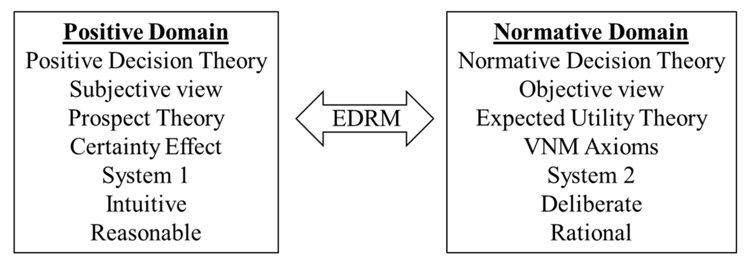
1. Introduction
1.1. A New Approach
1.2. Objectives
1.3. Definitions
2. Literature Review
3. Method
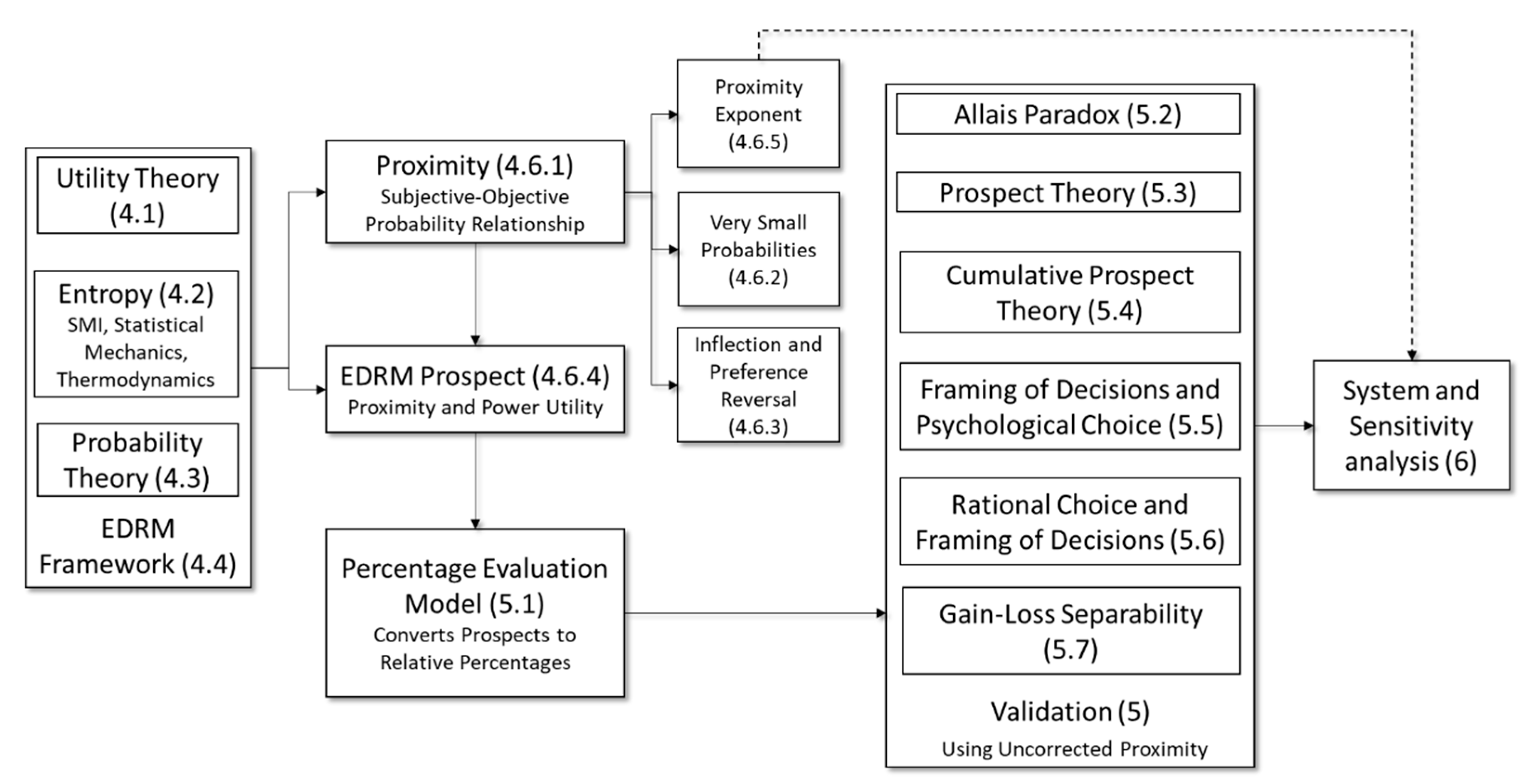
4. Derivation of EDRM: Theoretical Framework
4.1. Foundation of Utility Theory
4.2. Entropy
4.3. Two Types of Probabilities
4.4. Entropy Decision Risk Model (EDRM) Framework
- Certainty of gains and the uncertainty of losses are more highly valued;
- Gains and losses are considered contiguously as two regions of the same scale;
- Relative certainty, or redundancy, is one minus the relative entropy;
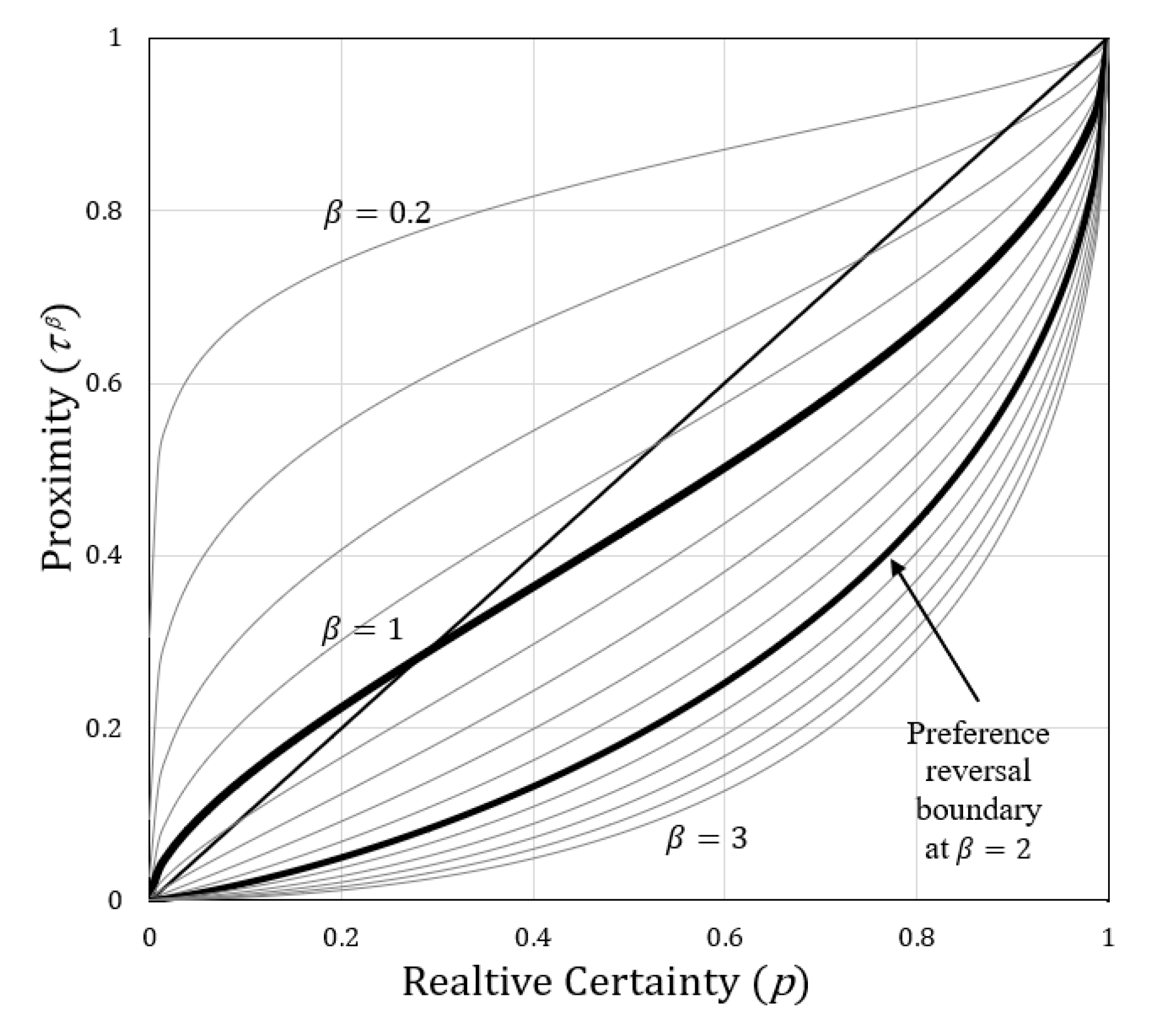
- Proximity is represented by the subjective probability of reaching a state;
- Prospect can be stated as magnitude times proximity as a function of relative certainty;
- The choice with the greatest prospect, positive or negative, is preferred.
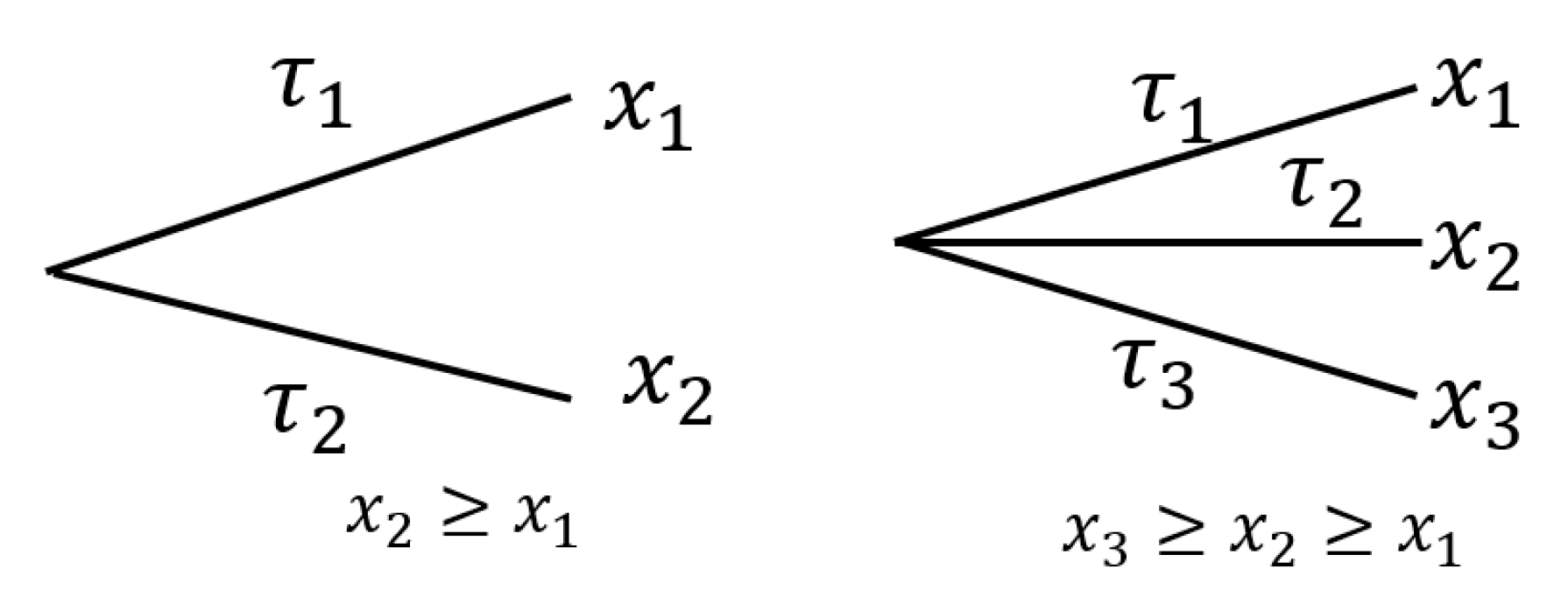
4.5. Choices and States
4.6. Prospect
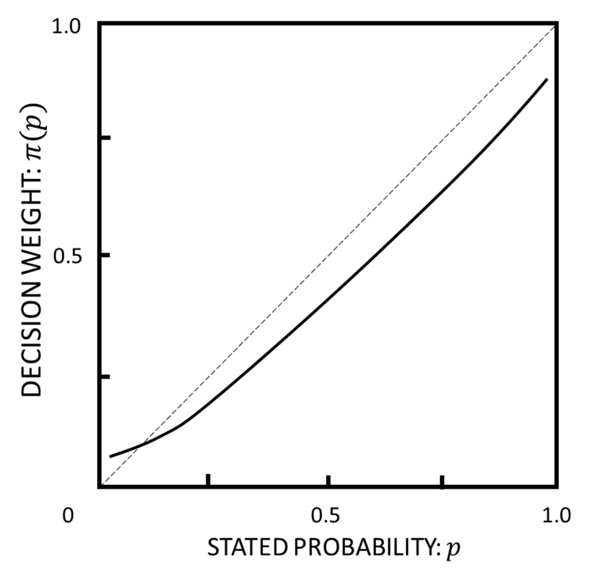
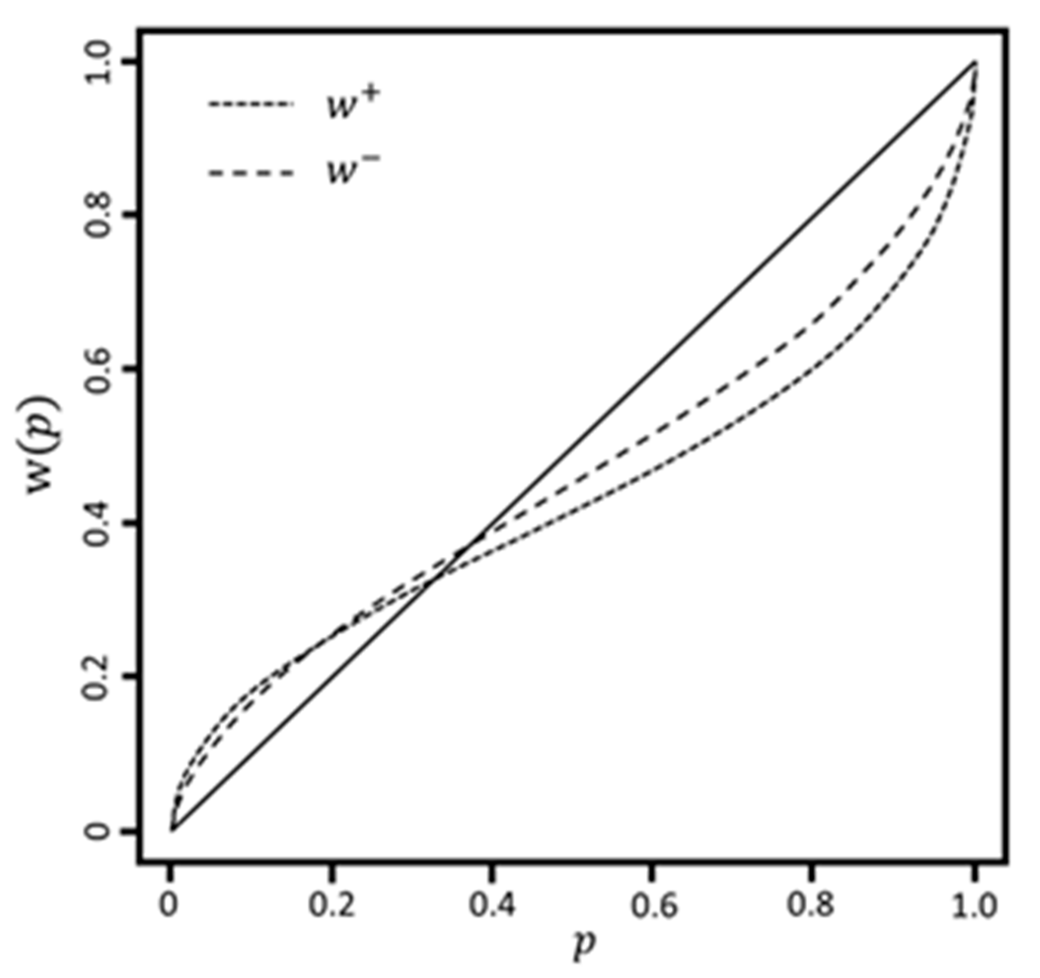
4.6.1. Derivation of Proximity from Information Theory Entropy (SMI) and Statistical Mechanics
4.6.2. Very Small Probabilities
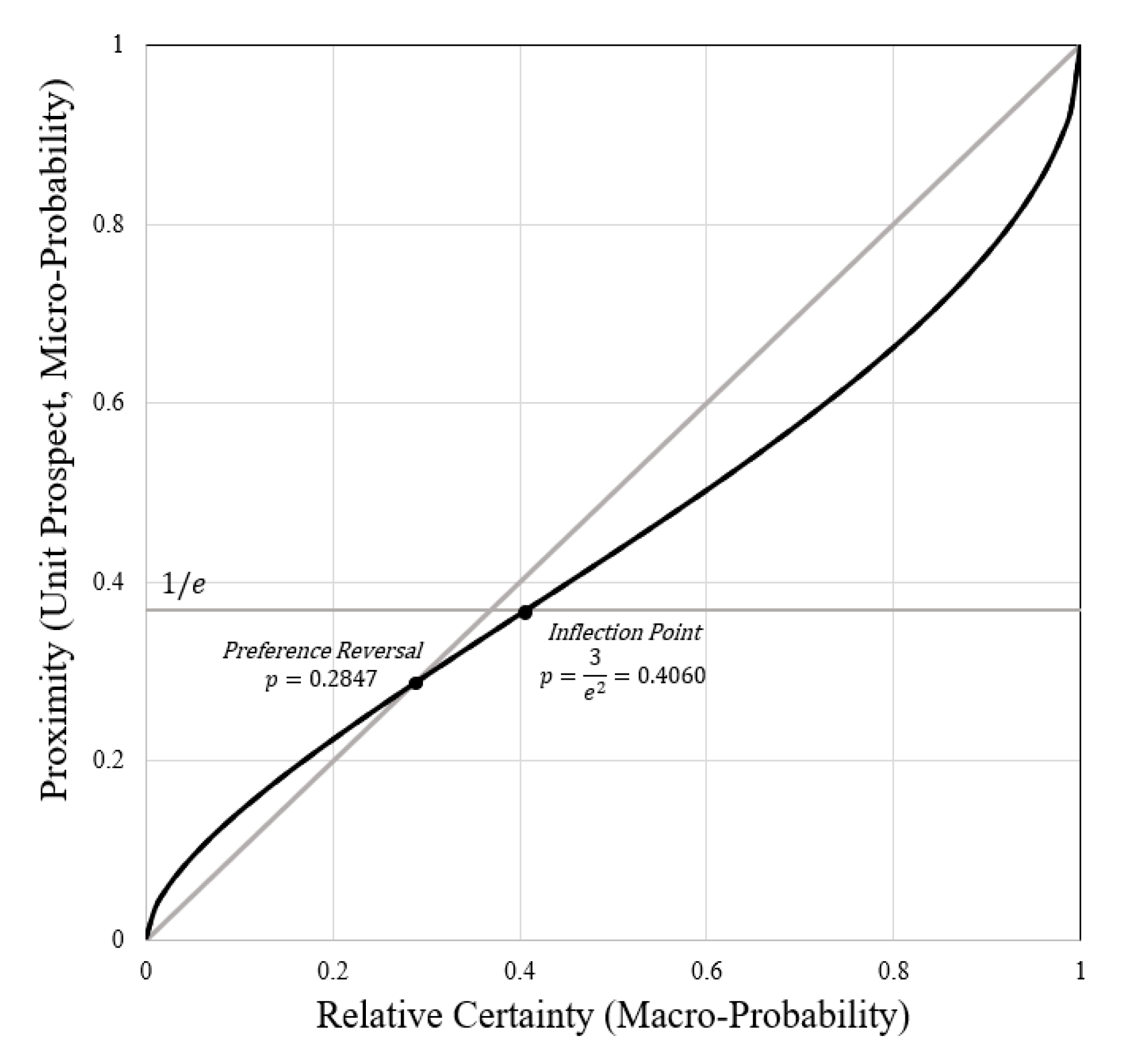
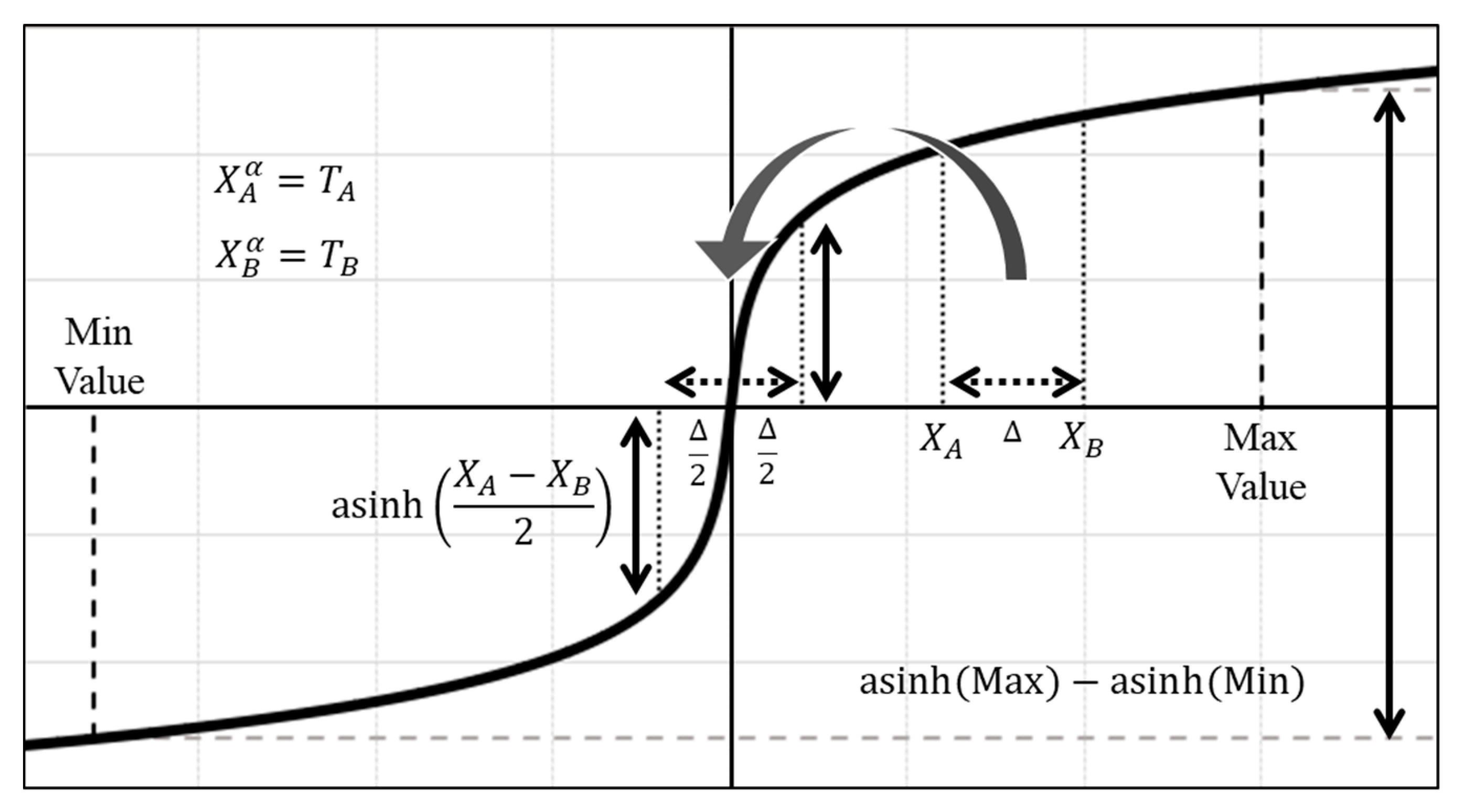
4.6.3. Inflection and Preference Reversal Points
4.6.4. Calculating Prospect of a Choice
4.6.5. Applying a Proximity Exponent () to the Prospect of a Choice
5. EDRM Validation (Without Application of Any Factors or Corrections, )
5.1. The Percentage Evaluation Model (PEM)
- Varies monotonically with the difference in prospect between choices;
- Scaled by the range, positive and negative, of values being evaluated in a given choice;
- Accounts for non-linearities of human perception;
- Equitably reports subject percentages for choices involving gains, losses, or mixtures of the two;
- Performs consistently across a range of studies (not tuned to a specific set of research).
5.2. Allais Paradox
5.3. Prospect Theory (Kahneman and Tversky)
5.4. Cumulative Prospect Theory
5.5. The Framing of Decisions and the Psychology of Choice (Tversky and Kahneman)
5.6. Rational Choice and the Framing of Decisions (Tversky and Kahneman)
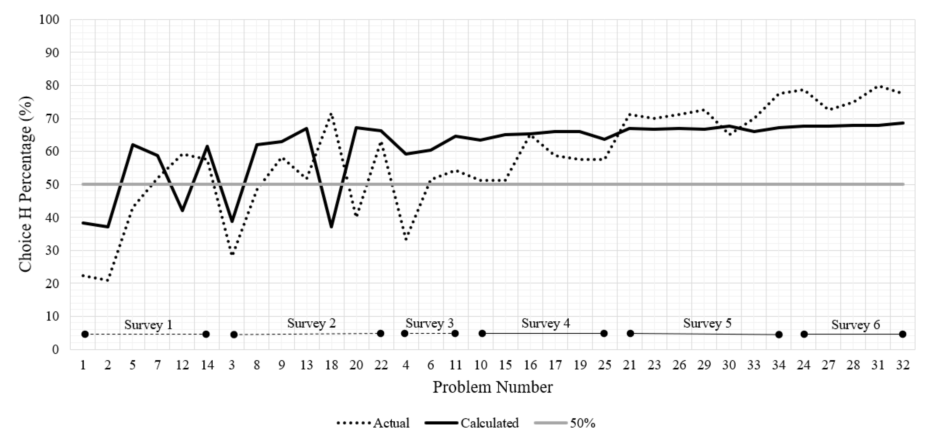
5.7. Gain-Loss Separability (Wu and Markle)
6. Summary of Analyses
System-Level Analysis of Choices (Sensitivity)
7. Discussion
Author Contributions
Funding
Conflicts of Interest
Appendix A. Derivation of Proximity from Entropy


Appendix B. Very Small Probabilities
Appendix C. Statistical Analyses
Appendix C.1. Percentage Evaluation Model

| Regression analysis: Coefficient of determination ( | ||||||
| Actual percentages compared with calculated for matching binary results only | 0.8026 | |||||
| Spearman rank correlation coefficient (Rho) | 0.8899 | |||||
| ANOVA (% actual vs. calculated) | Df | Sum Sq | Mean Sq | F-Value | Prob(>F) | Result |
| Study source | 7 | 517.8 | 73.977 | 0.8601 | 0.5401 | Not Significant |
| Type of choice (gain, loss, mix) | 2 | 96.0 | 48.005 | 0.8828 | 0.5737 | Not Significant |
| Interaction between source and type | 5 | 379.7 | 75.932 | 0.8828 | 0.4947 | Not Significant |
| Residuals | 128 | 11,009.5 | 86.012 | |||
| Normality Assumption | ||||||
| Shapiro–Wilk | W = 0.99522 | p-value = 0.9218 | Normal | |||
| Conclusions | ||||||
| 1. Cannot reject and null hypothesis, which means that the EDRM evaluation model is likely effective at expressing relative differences in prospect as percentages. Criteria 4 and 5 are met. 2. T-statistic test confirms no survey source is significant. | ||||||
Appendix C.2 Prospect Theory
| Binary matching (yes/no) (percentage) | 100% | |||||
| Regression analysis: Coefficient of determination () | ||||||
| Actual percentages compared with calculated (all match) | 0.8581 | |||||
| Spearman rank correlation coefficient (Rho) | 0.6966 | |||||
| ANOVA (% actual vs. calculated) | Df | Sum Sq | Mean Sq | F-Value | Prob(>F) | Result |
| Type of gamble (gain or loss) | 1 | 58.98 | 59.983 | 0.4648 | 0.5051 | Not Significant |
| # of Non-zero States (1 or 2) | 1 | 36.66 | 36.658 | 0.2889 | 0.5983 | Not Significant |
| Residuals | 15 | 2030.40 | 126.900 | |||
| Normality Assumption | ||||||
| Shapiro–Wilk | W = 0.94119 | p-value = 0.2771 | Normal | |||
| Conclusions | ||||||
| 1. Cannot reject any of the null hypotheses, which means that EDRM reasonably predicts results of Prospect Theory. | ||||||
Appendix C.3. Cumulative Prospect Theory
| Regression analysis: Coefficient of determination () | ||||||
| Actual values (not percentages) compared with calculated values | 0.9971 | |||||
| Actual values (not percentages) compared with calculated values (Positive only) | 0.9885 | |||||
| Actual values (not percentages) compared with calculated values (Negative only) | 0.9980 | |||||
| Spearman rank correlation coefficient (Rho) | 0.9982 | |||||
| ANOVA ( actual vs. calculated) | Df | Sum Sq | Mean Sq | F-Value | Prob(>F) | Result |
| Type of gamble (gain or loss) | 1 | 172.62 | 172.62 | 3.9040 | 0.05339 | Marginal |
| # Non-zero states (1 or 2) | 1 | 48.40 | 48.40 | 1.0946 | 0.30020 | Not significant |
| Residuals | 53 | 2343.49 | 44.217 | |||
| Normality Assumption | ||||||
| Shapiro–Wilk | W = 0.97213 | p-value = 0.2196 | Normal | |||
| Conclusions | ||||||
| 1. The coefficient of determination values for the comparison of actual and calculated values indicates near-perfect alignment and affirms Hypothesis 1. The ANOVA results for type of gamble do not reject the null hypothesis of no significant effect; however, the probability is very close to the 5% significance value indicating there is some difference between gains and losses, but that they can be considered as a secondary effect in this research given there is nearly no difference in the for positive (0.9885) and negative (0.9980) problems. Using a value of rather than 1 increases the type of gamble Prob(>F) to nearly 0.35 from 0.053. | ||||||
Appendix C.4. Wu and Markle Gain-Loss Separability
| Binary matching (yes/no) (percentage) | 82.3% | |||||
| Binomal test (Probability > 50%) | # Y:28, # Trials: 34 | p-value 1.95 × 10⁻⁴ | ||||
| Nonparametric analysis using Wilcoxon test | V = 206 | p-value 0.1207 | Agreement likely | |||
| Spearman rank correlation coefficient (Rho) | 0.6946 | |||||
| ANOVA(% actual vs. calc, matching only) | Df | Sum Sq | Mean Sq | F-Value | Prob(>F) | Result |
| Survey (6 surveys total) | 5 | 1602.40 | 320.48 | 8.7410 | 1.60 × 10⁻⁴ | Significant |
| Prospect signs (both pos, both neg, mix) | 2 | 66.56 | 33.28 | 0.9077 | 0.4194 | Not significant |
| Residuals | 20 | 733.28 | 36.66 | |||
| Normality Assumption | ||||||
| Shapiro–Wilk (All-including non-matching) | W = 0.81802 | p-value = 5.832 × 10⁻⁵ | Not normal | |||
| Shapiro–Wilk (matching binary result only) | W = 0.96881 | p-value = 0.5492 | Normal | |||
| Conclusions | ||||||
| 1. Wilcoxon null hypothesis cannot be rejected, so bias between calculated and actual values is unlikely. Additionally, this result further strengthens the PEM validation. 2. The sign of the resulting choice prospects has no significant effect. 3. The survey number is significant. All of the non-matching problems come from the surveys 1 through 3, which were conducted differently than surveys 4, 5, and 6; Survey 1 has a significantly higher difference mean than the other surveys. | ||||||
References
- von Neumann, J. Mathematical Foundations of Quantum Mechanics; Princeton University Press: Princeton, NJ, USA, 1955. [Google Scholar]
- DoD Risk, Issue, and Opportunity Management Guide for Defense Acquisition Programs; Department of Defense, Ed.; Office of the Deputy Assistant Secretary of Defense for Systems Engineering: Washington, DC, USA, 2017.
- DoD System Safety (MIL-STD-882E); Department of Defense, Ed.; Air Force Material Command, Wright-Patterson Air Force Base: Dayton, OH, USA, 2012.
- Monroe, T.J.; Beruvides, M.G. Risk, Entropy, and Decision-Making Under Uncertainty. In Proceedings of the 2018 IISE Annual Conference, Orlando, FL, USA, 19–22 May 2018. [Google Scholar]
- Kahneman, D. Thinking, Fast and Slow, 1st ed.; Farrar, Straus and Giroux: New York, NY, USA, 2011. [Google Scholar]
- Taleb, N.N. The Black Swan, 2nd ed.; Random House Trade Paperbacks: New York, NY, USA, 2010. [Google Scholar]
- Stanovich, K.E.; West, R.F. Individual differences in reasoning: Implications for the rationality debate? Behav. Brain Sci. 2000, 23, 645. [Google Scholar] [CrossRef] [PubMed]
- Schnieder, M. Dual Process Utility Theory: A Model of Decisions Under Risk and Over Time; Economic Science Institute, Chapman University, One University Drive: Orange, CA, USA, 2018. [Google Scholar]
- ISO. ISO 31000:2018 Risk Management—Guidelines; International Organization for Standardization: Geneva, Switzerland, 2018. [Google Scholar]
- Rasmussen, N. The Application of Probabilistic Risk Assessment Techniques to Energy Technologies. Annu. Rev. Energy 1981, 6, 123–138. [Google Scholar] [CrossRef]
- Tapiero, C.S. Risk and Financial Management; John Wiley and Sons Ltd.: West Sussex, UK, 2004. [Google Scholar]
- Ariely, D. Predictable Irrational: The Hidden Forces That Shape Our Decisions; HarperCollins: New York, NY, USA, 2009. [Google Scholar]
- Cohen, D. Homo Economicus, the (Lost) Prophet of Modern Times; Polity Press: Malden, MA, USA, 2014. [Google Scholar]
- Kahneman, D.; Tversky, A. Prospect Theory—Analysis of Decision under Risk. Econometrica 1979, 47, 263–291. [Google Scholar] [CrossRef]
- Markowitz, H. The Utility of Wealth. J. Polit. Econ. 1952, 60, 151–158. [Google Scholar] [CrossRef]
- Bernoulli, D. Exposition of a New Theory on the Measurement of Risk (1738). Econometrica 1954, 22, 23–36. [Google Scholar] [CrossRef]
- Tversky, A.; Kahneman, D. Advances in Prospect-Theory—Cumulative Representation of Uncertainty. J. Risk Uncertain. 1992, 5, 297–323. [Google Scholar] [CrossRef]
- Karmarkar, U.S. Subjectively weighted utility: A descriptive extension of the expected utility model. Organ. Behav. Hum. Perform. 1978, 21, 61–72. [Google Scholar] [CrossRef]
- Gonzalez, R.; Wu, G. On the Shape of the Probability Weighting Function. Cogn. Psychol. 1999, 38, 129–166. [Google Scholar] [CrossRef]
- Quiggin, J. A theory of anticipated utility. J. Econ. Behav. Organ. 1982, 3, 323–343. [Google Scholar] [CrossRef]
- Luce, R.; Ng, C.; Marley, A.; Aczél, J. Utility of gambling II: Risk, paradoxes, and data. Econ. Theory 2008, 36, 165–187. [Google Scholar] [CrossRef]
- Buchanan, A. Toward a Theory of the Ethics of Bureaucratic Organizations. Bus. Ethics Q. 1996, 6, 419–440. [Google Scholar] [CrossRef]
- Wakker, P.P.; Zank, H. A simple preference foundation of cumulative prospect theory with power utility. Eur. Econ. Rev. 2002, 46, 1253–1271. [Google Scholar] [CrossRef]
- Bentham, J. An Introduction to the Principles of Morals and Legislation; Kitchener, Ont.: Batoche, SK, Canada, 2000. [Google Scholar]
- Mill, J.S. Utilitarianism; Heydt, C., Ed.; Broadview Editions: Buffalo, NY, USA, 2011. [Google Scholar]
- Introduction to Aristotle; The Modern Library: New York, NY, USA, 1947.
- Ellsberg, D. Risk, Ambiguity, and the Savage Axioms. Q. J. Econ. 1961, 75, 643–669. [Google Scholar] [CrossRef]
- Wakker, P. Separating marginal utility and probabilistic risk aversion. Theory Decis. 1994, 36, 1–44. [Google Scholar] [CrossRef]
- Kahneman, D.; Wakker, P.P.W.; Sarin, R.S. Back to Bentham? Explorations of Experienced Utility. Q. J. Econ. 1997, 375. [Google Scholar] [CrossRef]
- Kahneman, D.; Thaler, R.H. Anomalies: Utility Maximization and Experienced Utility. J. Econ. Perspect. 2006, 20, 221–234. [Google Scholar] [CrossRef]
- Ben-Naim, A. Entropy and Information Theory: Uses and Misuses. Entropy 2019, 21, 1170. [Google Scholar] [CrossRef]
- Jaynes, E.T. Information Theory and Statistical Mechanics. Phys. Rev. 1957, 106, 620–630. [Google Scholar] [CrossRef]
- Boltzmann, L. Über die Mechanische Bedeutung des Zweiten Hauptsatzes der Wärmetheorie [On the Mechanical Importance of the Second Principles of Heat-Theory]. Wien. Ber. 1866, 53, 195–220. [Google Scholar]
- von Neumann, J.; Morgenstern, O. Theory of Games and Economic Behavior; Princeton University Press: Princeton, NJ, USA, 2007. [Google Scholar]
- Shannon, C.E.; Weaver, W. The Mathematical Theory of Communication; The Univeristy of Illinois Press: Urbana, IL, USA, 1949. [Google Scholar]
- Nawrocki, D.N.; Harding, W.H. State-Value Weighted Entropy as a Measure of Investment Risk. Appl. Econ. 1986, 18, 411–419. [Google Scholar] [CrossRef]
- Yang, J.; Qiu, W. Normalized Expected Utility-Entropy Measure of Risk. Entropy 2014, 16, 3590–3604. [Google Scholar] [CrossRef]
- Belavkin, R.V. Asymmetry of Risk and Value of Information; Middlesex University: London, UK, 2014. [Google Scholar] [CrossRef]
- Belavkin, R.; Ritter, F.E. The Use of Entropy for Analysis and Control of Cognitive Models. In Proceedings of the Fifth International Conference on Cognitive Modeling, Bamberg, Germany, 9–12 April 2003; pp. 21–26. [Google Scholar]
- Tversky, A. Preference, Belief, and Similarity; The MIT Press: Cambridge, MA, USA, 2004. [Google Scholar]
- Hellman, Z.; Peretz, R. A Survey on Entropy and Economic Behaviour. Entropy 2020, 22, 157. [Google Scholar] [CrossRef]
- Zingg, C.; Casiraghi, G.; Vaccario, G.; Schweitzer, F. What Is the Entropy of a Social Organization? Entropy 2019, 21, 901. [Google Scholar] [CrossRef]
- Pisano, R.; Sozzo, S. A Unified Theory of Human Judgements and Decision-Making under Uncertainty. Entropy 2020, 22, 738. [Google Scholar] [CrossRef]
- Keynes, J.M. A Treatise on Probability; Macmillan and Co., Limited: London, UK, 1921. [Google Scholar]
- Hume, D. A Treatise of Human Nature: Being an Attempt to Introduce the Experimental Method of Reasoning into Moral Subjects; Batoche Books Limited: Kitchener, ON, Canada, 1998. [Google Scholar]
- Jaynes, E.T. Probability Theory: The Logic of Science; Bretthorst, G.L., Ed.; Cambridge University Press: Cambridge, UK; New York, NY, USA, 2003. [Google Scholar]
- Waismann, F. Logische Analyse des Wahrscheinlichkeitsbegriffs. Erkenntnis 1930, 1, 228. [Google Scholar] [CrossRef]
- Carnap, R. The Two Concepts of Probability: The Problem of Probability. Philos. Phenomenol. Res. 1945, 5, 513–532. [Google Scholar] [CrossRef]
- Abdellaoui, M. Uncertainty and Risk: Mental, Formal, Experimental Representations; Springer: Berlin/Heidelberg, Germany; London, UK, 2007. [Google Scholar]
- Tversky, A.; Kahneman, D. Judgment under Uncertainty: Heuristics and Biases. Science 1974, 185, 1124–1131. [Google Scholar] [CrossRef]
- Bayes, T.; Price, R. An Essay towards Solving a Problem in the Doctrine of Chances. By the Late Rev. Mr. Bayes, F.R.S. Communicated by Mr. Price, in a Letter to John Canton, A.M.F.R.S. Philos. Trans. (1683–1775) 1763, 53, 370–418. [Google Scholar]
- Frigg, R. Probability in Boltzmannian Statistical Mechanics. In Time, Chance and Reduction. Philosophical Aspects of Statistical Mechanics; Gerhard Ernst, G., Huttemann, A., Eds.; Cambridge University Press: Cambridge, UK, 2010. [Google Scholar]
- Waismann, F. Philosophical Papers; D. Reidel Pub. Co.: Dordrecht, The Netherlands, 1977. [Google Scholar]
- Popper, K. The Logic of Scientific Discovery; Routledge: London, UK; New York, NY, USA, 1992. [Google Scholar]
- Shackle, G.L.S. Expectation in Economics, 2nd ed.; Cambridge University Press: Cambridge, UK, 1952. [Google Scholar]
- ANSI/ASSE/ISO 31000-2009. Risk Management Principles and Guidelines; American Society of Safety Engineers: Des Plaines, IL, USA, 2011. [Google Scholar]
- Prelec, D. The Probability Weighting Function. Econometrica 1998, 66, 497–527. [Google Scholar] [CrossRef]
- Wu, G.; Gonzalez, R. Curvature of the Probability Weighting Function. Manag. Sci. 1996, 42, 1676–1690. [Google Scholar] [CrossRef]
- Lichtenstein, S.; Slovic, P. Reversals of preference between bids and choices in gambling decisions. J. Exp. Psychol. 1971, 89, 46–55. [Google Scholar] [CrossRef]
- Tversky, A.; Sattath, S.; Slovic, P. Contingent Weighting in Judgment and Choice. Psychol. Rev. 1988, 95, 371–384. [Google Scholar] [CrossRef]
- Schumpeter, J.A. History of Economic Analysis; Oxford University Press: New York, NY, USA, 1954. [Google Scholar]
- Tversky, A.; Kahneman, D. The framing of decisions and the psychology of choice. Science 1981, 211, 453. [Google Scholar] [CrossRef] [PubMed]
- Tversky, A.; Kahneman, D. Rational choice and the framing of decisions. J. Bus. 1986, 59, S251. [Google Scholar] [CrossRef]
- Birnbaum, M.H. Three New Tests of Independence That Differentiate Models of Risky Decision Making. Manag. Sci. 2005, 51, 1346–1358. [Google Scholar] [CrossRef]
- Birnbaum, M.H.; Bahra, J.P. Gain-loss separability and coalescing in risky decision making. Manag. Sci. 2007, 53, 1016–1028. [Google Scholar] [CrossRef][Green Version]
- Prelec, D. A “Pseudo-endowment” effect, and its implications for some recent nonexpected utility models. J. Risk Uncertain. 1990, 3, 247–259. [Google Scholar] [CrossRef]
- Wu, G.; Markle, A.B. An Empirical Test of Gain-Loss Separability in Prospect Theory. Manag. Sci. 2008, 54, 1322–1335. [Google Scholar] [CrossRef]
- Allais, M. An Outline of My Main Contributions to Economic Science. Am. Econ. Rev. 1997, 87, 3–12. [Google Scholar] [CrossRef]
- Allais, M. Le Comportement de l’Homme Rationnel devant le Risque: Critique des Postulats et Axiomes de l’Ecole Americaine. Econometrica 1953, 21, 503–546. [Google Scholar] [CrossRef]
- Machina, M.J. Choice Under Uncertainty: Problems Solved and Unsolved. J. Econ. Perspect. 1987, 1, 121–154. [Google Scholar] [CrossRef]
- Conlisk, J. The Utility of Gambling. J. Risk Uncertain. 1993, 6, 255–275. [Google Scholar] [CrossRef]
- Thaler, R.H. Transaction Utility Theory. Adv. Consum. Res. 1983, 10, 229–232. [Google Scholar]
- Hoseinzadeh, A.; Mohtashami Borzadaran, G.; Yari, G. Aspects concerning entropy and utility. Theory Decis. 2012, 72, 273–285. [Google Scholar] [CrossRef]
| 1 | The factors used in equations by Gonzalez and Wu () are not those used in EDRM but are quoted in their original form for accuracy. Additionally, this relationship is nearly identical to that stated by Karmarkar. |
| 2 | As this paper is focused upon the application of an entropy model for positive decision theories, the apparent isomorphology between Boltzmann’s Principle and Daniel Bernoulli’s expected utility theory will be more deeply addressed in subsequent research. |
| 3 | This case is identical to that of the classical or frequency definition of probability, where each state is assumed to have to same probability due to a lack of knowledge about the states. |
| 4 | The Authors have chosen to use T out of respect for Amos Tversky who passed before being awarded the Nobel Prize alongside Daniel Kahneman. |
| 5 | Prelec’s relationship is provided as written; however, the constant is not the same as that used for power utility. |
| 6 | To separate decision weights in the two-value CPT actual data, the following was assumed: . |


| Problem (Value, Probability) | EDRM | Calc % | Match | ||||
|---|---|---|---|---|---|---|---|
| Choice A (1 and 3) | Choice B (2 and 4) | A | B | Y/N | |||
| 1 and 2 | (1M) | (5M, 0.10; 1M, 0.89) | 190,456 | 131,265 | 90 | 10 | Yes |
| 3 and 4 | (5M,.10) | (1M,.11) | 112,312 | 28,925 | 90 | 10 | Yes |
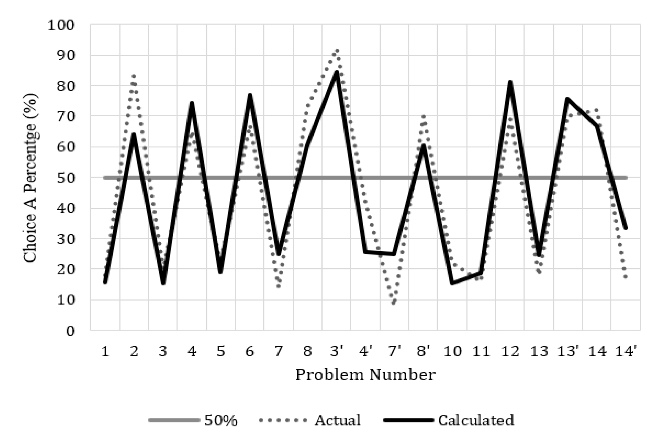
| Problem | EDRM | Calc % | Actual % | Diff | ||||||
|---|---|---|---|---|---|---|---|---|---|---|
| Choice A | Choice B | A | B | A | B | Δ% | ||||
| 1 | (2500, 0.33; 2400, 0.66) | (2400) | 824.66 | 943.16 | 16 | 84 | 18 | 82 | 2 | |
| 2 | (2500, 0.33) | (2400, 0.34) | 308.94 | 304.55 | 64 | 36 | 83 | 17 | 19 | |
| 3 | (4000, 0.8) | (3000) | 978.90 | 1147.80 | 15 | 85 | 20 | 80 | 5 | |
| 4 | (4000, 0.2) | (3000, 0.25) | 330.73 | 298.54 | 74 | 26 | 65 | 35 | −9 | |
| 5 | (10000, 0.5) | (4320)1 1 | 1430.49 | 1582.07 | 19 | 81 | 22 | 78 | 3 | |
| 6 | (10000, 0.05) | (4320, 0.1) 1 | 308.95 | 226.24 | 77 | 23 | 67 | 33 | −10 | |
| 7 | (6000, 0.45) | (3000, 0.9) | 840.31 | 879.79 | 25 | 75 | 14 | 86 | −11 | |
| 8 | (6000, 0.001) | (3000, 0.002) | 20.70 | 16.64 | 60 | 40 | 73 | 27 | 13 | |
| 3′ | (−4000, 0.8) | (−3000) | −978.90 | −1147.80 | 85 | 15 | 92 | 8 | 7 | |
| 4′ | (−4000, 0.2) | (−3000, 0.25) | −330.73 | −298.54 | 26 | 74 | 42 | 58 | 16 | |
| 7′ | (−3000, 0.9) | (−6000, 0.45) | −879.79 | −840.31 | 25 | 75 | 8 | 92 | −17 | |
| 8′ | (−3000, 0.002) | (−6000, 0.001) | −16.64 | −20.70 | 60 | 40 | 70 | 30 | 10 | |
| 10 2 | (4000, 0.8) | (3000) | 978.90 | 1147.80 | 15 | 85 | 22 | 78 | 7 | |
| 11 | (1000, 0.5) | (500) | 188.57 | 237.19 | 19 | 81 | 16 | 84 | −3 | |
| 12 | (−1000, 0.5) | (−500) | −188.57 | −237.19 | 81 | 19 | 69 | 31 | −12 | |
| 13 | (6000, 0.25) | (4000, 0.25; 2000, 0.25) | 549.43 | 593.50 | 25 | 75 | 18 | 82 | −7 | |
| 13′ | (−6000, 0.25) | (−4000, 0.25;−2000, 0.25) | −549.43 | −593.50 | 75 | 25 | 70 | 30 | −5 | |
| 14 | (5000, 0.001) | (5) | 17.63 | 4.12 | 67 | 33 | 72 | 28 | 5 | |
| 14′ | (−5000, 0.001) | (−5) | −17.63 | −4.12 | 33 | 67 | 17 | 83 | 2 | |
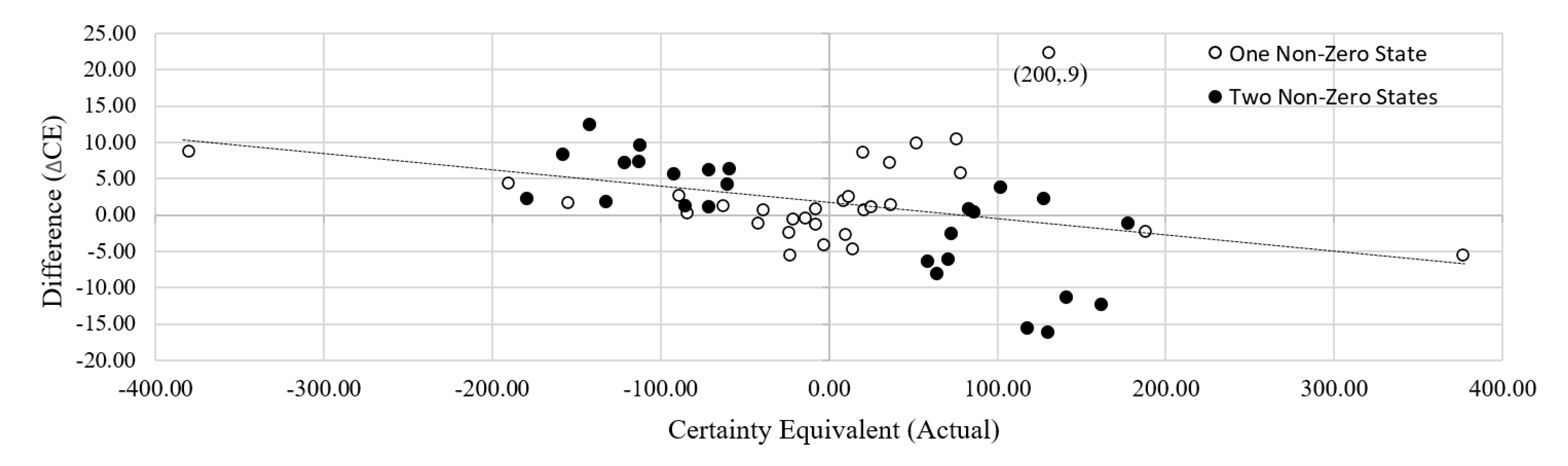
| Problem | EDRM | Results | ||||
|---|---|---|---|---|---|---|
| Outcomes | Gamble | Actual CE | Diff Δ CE | |||
| (0, 50) | (50, 0.1) | 0.1430 | 7.15 | 9 | 1.85 | |
| (50, 0.5) | 0.4320 | 21.60 | 21 | 0.6 | ||
| (50, 0.9) | 0.7665 | 38.32 | 37 | 1.325 | ||
| (0, −50) | (−50, 0.1) | 0.1430 | −7.15 | −8 | 0.85 | |
| (−50, 0.5) | 0.4320 | −21.60 | −21 | −0.6 | ||
| (−50, 0.9) | 0.7665 | −38.32 | −39 | 0.675 | ||
| (0, 100) | (100, 0.005) | 0.0933 | 9.33 | 14 | −4.67 | |
| (100, 0.25) | 0.2601 | 26.01 | 25 | 1.01 | ||
| (100, 0.5) | 0.4320 | 43.20 | 36 | 7.2 | ||
| (100, 0.75) | 0.6183 | 61.83 | 52 | 9.83 | ||
| (100, 0.95) | 0.8372 | 83.72 | 78 | 5.72 | ||
| (0, −100) | (−100, 0.005) | 0.0933 | −9.33 | −8 | −1.33 | |
| (−100, 0.25) | 0.2601 | −26.01 | −23.5 | −2.51 | ||
| (−100, 0.5) | 0.4320 | −43.20 | −42 | −1.2 | ||
| (−100, 0.75) | 0.6183 | −61.83 | −63 | 1.17 | ||
| (−100, 0.95) | 0.8372 | −83.72 | −84 | 0.28 | ||
| (0, 200) | (200, 0.01) | 0.0361 | 7.22 | 10 | −2.78 | |
| (200, 0.1) | 0.1430 | 28.60 | 20 | 8.6 | ||
| (200, 0.5) | 0.4320 | 86.40 | 76 | 10.4 | ||
| (200, 0.9) | 0.7665 | 153.30 | 131 | 22.3 | ||
| (200, 0.99) | 0.9284 | 185.68 | 188 | −2.32 | ||
| (0, −200) | (−200, 0.01) | 0.0361 | −7.22 | −3 | −4.22 | |
| (−200, 0.1) | 0.1430 | −28.60 | −23 | −5.6 | ||
| (−200, 0.5) | 0.4320 | −86.40 | −89 | 2.6 | ||
| (−200, 0.9) | 0.7665 | −153.30 | −155 | 1.7 | ||
| (−200, 0.99) | 0.9284 | −185.68 | −190 | 4.32 | ||
| (0, 400) | (400, 0.01) | 0.0361 | 14.44 | 12 | 2.44 | |
| (400, 0.99) | 0.9284 | 371.36 | 377 | −5.64 | ||
| (0, −400) | (−400, 0.01) | 0.0361 | −14.44 | −14 | −0.44 | |
| (−400, 0.99) | 0.9284 | −371.36 | −380 | 8.64 | ||
| (50, 100) | (50, 0.9; 100, 0.1) | 0.1430 | 0.7665 | 52.62 | 59 | −6.375 |
| (50, 0.5; 100, 0.5) | 0.4320 | 0.4320 | 64.80 | 71 | −6.2 | |
| (50, 0.1; 100, 0.9) | 0.7665 | 0.1430 | 83.80 | 83 | 0.8 | |
| (−50, −100) | (−50, 0.9; −100, 0.1) | 0.1430 | 0.7665 | −52.62 | −59 | 6.375 |
| (−50, 0.5; −100, 0.5) | 0.4320 | 0.4320 | −64.80 | −71 | 6.2 | |
| (−50, 0.1; −100, 0.9) | 0.7665 | 0.1430 | −83.80 | −85 | 1.2 | |
| (50, 150) | (50, 0.95; 150, 0.05) | 0.0933 | 0.8372 | 55.85 | 64 | −8.145 |
| (50, 0.75; 150, 0.25) | 0.2601 | 0.6183 | 69.93 | 72.5 | −2.57 | |
| (50, 0.5; 150, 0.5) | 0.4320 | 0.4320 | 86.40 | 86 | 0.4 | |
| (50, 0.25; 150, 0.75) | 0.6183 | 0.2601 | 105.75 | 102 | 3.75 | |
| (50, 0.05;150, 0.95) | 0.8372 | 0.0933 | 130.24 | 128 | 2.245 | |
| (−50, −150) | (−50, 0.95; −150, 0.05) | 0.0933 | 0.8372 | −55.85 | −60 | 4.145 |
| (−50, 0.75; −150, 0.25) | 0.2601 | 0.6183 | −69.93 | −71 | 1.07 | |
| (−50, 0.5; −150, 0.5) | 0.4320 | 0.4320 | −86.40 | −92 | 5.6 | |
| (−50, 0.25; −150, 0.75) | 0.6183 | 0.2601 | −105.75 | −113 | 7.25 | |
| (−50, 0.05; −150, 0.95) | 0.8372 | 0.0933 | −130.24 | −132 | 1.755 | |
| (100, 200) | (100, 0.95; 200, 0.05) | 0.0933 | 0.8372 | 102.38 | 118 | −15.62 |
| (100, 0.75; 200, 0.25) | 0.2601 | 0.6183 | 113.85 | 130 | −16.15 | |
| (100, 0.5; 200, 0.5) | 0.4320 | 0.4320 | 129.60 | 141 | −11.4 | |
| (100, 0.25; 200, 0.75) | 0.6183 | 0.2601 | 149.67 | 162 | −12.33 | |
| (100, 0.05; 200, 0.95) | 0.8372 | 0.0933 | 176.77 | 178 | −1.23 | |
| (−100, −200) | (−100, 0.95; −200, 0.05) | 0.0933 | 0.8372 | −102.38 | −112 | 9.62 |
| (−100, 0.75; −200, 0.25) | 0.2601 | 0.6183 | −113.85 | −121 | 7.15 | |
| (−100, 0.5; −200, 0.5) | 0.4320 | 0.4320 | −129.60 | −142 | 12.4 | |
| (−100, 0.25; −200, 0.75) | 0.6183 | 0.2601 | −149.67 | −158 | 8.33 | |
| (−100, 0.05; −200, 0.95) | 0.8372 | 0.0933 | −176.77 | −179 | 2.23 | |
| Problem (Value, Probability) | EDRM | Calc % | Actual % | Diff | Match | |||||
|---|---|---|---|---|---|---|---|---|---|---|
| Choice A | Choice B | A | B | A | B | Δ% | Y/N | |||
| 1 | (200) | (600, 1/3) | 106 | 89 | 75 | 25 | 72 | 28 | −3 | Yes |
| 2 | (−400) | (0, 1/3; −600, 2/3) | −195 | −154 | 18 | 82 | 22 | 78 | 4 | Yes |
| 3i | (240) | (1000, 0.25) | 124 | 114 | 71 | 29 | 84 | 16 | 13 | Yes |
| 3ii | (−750) | (−1000, 0.75) | −339 | −270 | 16 | 84 | 13 | 87 | −3 | Yes |
| 4 | (240, 0.25; −760, 0.75) | (250, 0.25; −750, 0.75) | −180 | −176 | 0 | 100 2 | 0 | 100 | 0 | Yes |
| 5 | (30) | (45,.8) | 20 | 19 | 59 | 41 | 78 | 22 | 19 | Yes |
| 6 1 | (30) | (45,.8) | 20 | 19 | 59 | 41 | 74 | 26 | 15 | Yes |
| 7 | (30,.25) | (45,.2) | 5.2 | 6.4 | 41 | 59 | 42 | 58 | 1 | Yes |
| Problem (Value, Probability) | EDRM | Calc % | Actual % | Diff | Match | |||||
|---|---|---|---|---|---|---|---|---|---|---|
| Choice A | Choice B | A | B | A | B | Δ% | Y/N | |||
| 7 | (0, 0.9; 45, 0.06; 30, 0.01;−15, 0.01; −15, 0.02) | (0, 0.9; 45, 0.06; 45, 0.01;−10, 0.01, −15, 0.02) | 2.71 | 3.14 | 0 | 100 1 | 0 | 100 | 0 | Yes |
| 8 | (0, 0.9; 45, 0.06, 30, 0.01; −15, 0.03) | (0, 0.9; 45, 0.07; −10, 0.01,− 15, 0.02) | 2.95 | 2.40 | 52 | 48 | 58 | 42 | 6 | Yes |
| Choice H | Choice L | Proximity | Prospect | Results (%) | ||||||||||||||||
|---|---|---|---|---|---|---|---|---|---|---|---|---|---|---|---|---|---|---|---|---|
| Calc | Actual | Eval | ||||||||||||||||||
| H | L | H | L | Δ% | Y/N | |||||||||||||||
| 1 | 150 | 0.3 | −25 | 0.7 | 75 | 0.8 | −60 | 0.2 | 0.30 | 0.58 | 0.66 | 0.22 | 14 | 21 | 38 | 62 | 22 | 78 | −16 | Y |
| 2 | 1800 | 0.05 | −200 | 0.95 | 600 | 0.3 | −250 | 0.7 | 0.09 | 0.84 | 0.30 | 0.58 | −20 | 8 | 37 | 63 | 21 | 79 | −16 | Y |
| 3 | 1000 | 0.25 | −500 | 0.75 | 600 | 0.5 | −700 | 0.5 | 0.26 | 0.62 | 0.43 | 0.43 | −33 | −17 | 39 | 61 | 28 | 72 | −11 | Y |
| 4 | 200 | 0.3 | −25 | 0.7 | 75 | 0.8 | −100 | 0.2 | 0.30 | 0.58 | 0.66 | 0.22 | 21 | 17 | 59 | 41 | 33 | 67 | −26 | N |
| 5 | 1200 | 0.25 | −500 | 0.75 | 600 | 0.5 | −800 | 0.5 | 0.26 | 0.62 | 0.43 | 0.43 | −13 | −35 | 62 | 38 | 43 | 57 | −19 | N |
| 6 | 750 | 0.4 | −1000 | 0.6 | 500 | 0.6 | −1500 | 0.4 | 0.36 | 0.50 | 0.50 | 0.36 | −96 | −108 | 60 | 40 | 51 | 49 | −9 | Y |
| 7 | 4200 | 0.5 | −3000 | 0.5 | 3000 | 0.75 | −6000 | 0.25 | 0.43 | 0.43 | 0.62 | 0.26 | 171 | 160 | 59 | 41 | 52 | 48 | −7 | Y |
| 8 | 4500 | 0.5 | −1500 | 0.5 | 3000 | 0.75 | −3000 | 0.25 | 0.43 | 0.43 | 0.62 | 0.26 | 439 | 411 | 62 | 38 | 48 | 52 | −14 | N |
| 9 | 4500 | 0.5 | −3000 | 0.5 | 3000 | 0.75 | −6000 | 0.25 | 0.43 | 0.43 | 0.62 | 0.26 | 213 | 160 | 63 | 37 | 58 | 42 | −5 | Y |
| 10 | 1000 | 0.3 | −200 | 0.7 | 400 | 0.7 | −500 | 0.3 | 0.30 | 0.58 | 0.58 | 0.30 | 68 | 43 | 63 | 37 | 51 | 49 | −12 | Y |
| 11 | 4800 | 0.5 | −1500 | 0.5 | 3000 | 0.75 | −3000 | 0.25 | 0.43 | 0.43 | 0.62 | 0.26 | 480 | 411 | 65 | 35 | 54 | 46 | −10 | Y |
| 12 | 3000 | 0.01 | −490 | 0.99 | 2000 | 0.02 | −500 | 0.98 | 0.04 | 0.93 | 0.05 | 0.90 | −175 | −170 | 42 | 58 | 59 | 41 | 17 | N |
| 13 | 2200 | 0.4 | −600 | 0.6 | 850 | 0.75 | −1700 | 0.25 | 0.36 | 0.50 | 0.62 | 0.26 | 178 | 53 | 67 | 33 | 52 | 48 | −15 | Y |
| 14 | 2200 | 0.2 | −1000 | 0.8 | 1700 | 0.25 | −1100 | 0.75 | 0.22 | 0.66 | 0.26 | 0.62 | −94 | −112 | 61 | 39 | 58 | 42 | −4 | Y |
| 15 | 1500 | 0.25 | −500 | 0.75 | 600 | 0.5 | −900 | 0.5 | 0.26 | 0.62 | 0.43 | 0.43 | 16 | −52 | 65 | 35 | 51 | 49 | −14 | Y |
| 16 | 5000 | 0.5 | −3000 | 0.5 | 3000 | 0.75 | −6000 | 0.25 | 0.43 | 0.43 | 0.62 | 0.26 | 281 | 160 | 65 | 35 | 65 | 35 | 0 | Y |
| 17 | 1500 | 0.4 | −1000 | 0.6 | 600 | 0.8 | −3500 | 0.2 | 0.36 | 0.50 | 0.66 | 0.22 | 8 | −110 | 66 | 34 | 59 | 41 | −7 | Y |
| 18 | 2025 | 0.5 | −875 | 0.5 | 1800 | 0.6 | −1000 | 0.4 | 0.43 | 0.43 | 0.50 | 0.36 | 183 | 209 | 37 | 63 | 72 | 28 | 35 | N |
| 19 | 600 | 0.25 | −100 | 0.75 | 125 | 0.75 | −500 | 0.25 | 0.26 | 0.62 | 0.62 | 0.26 | 37 | −18 | 66 | 34 | 58 | 43 | −8 | Y |
| 20 | 5000 | 0.1 | −900 | 0.9 | 1400 | 0.3 | −1700 | 0.7 | 0.14 | 0.77 | 0.30 | 0.58 | −48 | −229 | 67 | 33 | 40 | 60 | −27 | N |
| 21 | 700 | 0.25 | −100 | 0.75 | 125 | 0.75 | −600 | 0.25 | 0.26 | 0.62 | 0.62 | 0.26 | 47 | −29 | 67 | 33 | 71 | 29 | 4 | Y |
| 22 | 700 | 0.5 | −150 | 0.5 | 350 | 0.75 | −400 | 0.25 | 0.43 | 0.43 | 0.62 | 0.26 | 102 | 56 | 66 | 34 | 63 | 37 | −3 | Y |
| 23 | 1200 | 0.3 | −200 | 0.7 | 400 | 0.7 | −800 | 0.3 | 0.30 | 0.58 | 0.58 | 0.30 | 90 | 7 | 67 | 33 | 70 | 30 | 3 | Y |
| 24 | 5000 | 0.5 | −2500 | 0.5 | 2500 | 0.75 | −6000 | 0.25 | 0.43 | 0.43 | 0.62 | 0.26 | 355 | 55 | 68 | 32 | 79 | 21 | 11 | Y |
| 25 | 800 | 0.4 | −1000 | 0.6 | 500 | 0.6 | −1600 | 0.4 | 0.36 | 0.50 | 0.50 | 0.36 | −89 | −121 | 64 | 36 | 58 | 43 | −6 | Y |
| 26 | 5000 | 0.5 | −3000 | 0.5 | 2500 | 0.75 | −6500 | 0.25 | 0.43 | 0.43 | 0.62 | 0.26 | 281 | 15 | 67 | 33 | 71 | 29 | 4 | Y |
| 27 | 700 | 0.25 | −100 | 0.75 | 100 | 0.75 | −800 | 0.25 | 0.26 | 0.62 | 0.62 | 0.26 | 47 | −58 | 68 | 32 | 73 | 28 | 5 | Y |
| 28 | 1500 | 0.3 | −200 | 0.7 | 400 | 0.7 | −1000 | 0.3 | 0.30 | 0.58 | 0.58 | 0.30 | 123 | −16 | 68 | 32 | 75 | 25 | 7 | Y |
| 29 | 1600 | 0.25 | −500 | 0.75 | 600 | 0.5 | −1100 | 0.5 | 0.26 | 0.62 | 0.43 | 0.43 | 25 | −85 | 67 | 33 | 73 | 28 | 6 | Y |
| 30 | 2000 | 0.4 | −800 | 0.6 | 600 | 0.8 | −3500 | 0.2 | 0.36 | 0.50 | 0.66 | 0.22 | 112 | −110 | 68 | 32 | 65 | 35 | −3 | Y |
| 31 | 2000 | 0.25 | −400 | 0.75 | 600 | 0.5 | −1100 | 0.5 | 0.26 | 0.62 | 0.43 | 0.43 | 88 | −85 | 68 | 32 | 80 | 20 | 12 | Y |
| 32 | 1500 | 0.4 | −700 | 0.6 | 300 | 0.8 | −3500 | 0.2 | 0.36 | 0.50 | 0.66 | 0.22 | 67 | −194 | 69 | 31 | 78 | 23 | 9 | Y |
| 33 | 900 | 0.4 | −1000 | 0.6 | 500 | 0.6 | −1800 | 0.4 | 0.36 | 0.50 | 0.50 | 0.36 | −75 | −147 | 66 | 34 | 70 | 30 | 4 | Y |
| 34 | 1000 | 0.4 | −1000 | 0.6 | 500 | 0.6 | −2000 | 0.4 | 0.36 | 0.50 | 0.50 | 0.36 | −61 | −173 | 67 | 33 | 78 | 23 | 10 | Y |
Publisher’s Note: MDPI stays neutral with regard to jurisdictional claims in published maps and institutional affiliations. |
© 2020 by the authors. Licensee MDPI, Basel, Switzerland. This article is an open access article distributed under the terms and conditions of the Creative Commons Attribution (CC BY) license (http://creativecommons.org/licenses/by/4.0/).
Share and Cite
Monroe, T.; Beruvides, M.; Tercero-Gómez, V. Derivation and Application of the Subjective–Objective Probability Relationship from Entropy: The Entropy Decision Risk Model (EDRM). Systems 2020, 8, 46. https://doi.org/10.3390/systems8040046
Monroe T, Beruvides M, Tercero-Gómez V. Derivation and Application of the Subjective–Objective Probability Relationship from Entropy: The Entropy Decision Risk Model (EDRM). Systems. 2020; 8(4):46. https://doi.org/10.3390/systems8040046
Chicago/Turabian StyleMonroe, Thomas, Mario Beruvides, and Víctor Tercero-Gómez. 2020. "Derivation and Application of the Subjective–Objective Probability Relationship from Entropy: The Entropy Decision Risk Model (EDRM)" Systems 8, no. 4: 46. https://doi.org/10.3390/systems8040046
APA StyleMonroe, T., Beruvides, M., & Tercero-Gómez, V. (2020). Derivation and Application of the Subjective–Objective Probability Relationship from Entropy: The Entropy Decision Risk Model (EDRM). Systems, 8(4), 46. https://doi.org/10.3390/systems8040046