1. Introduction
It is well known, and well established by experimental observations, that systems characterized by observable ordered symmetry patterns, such as crystal, ferromagnets, superconductors, may be described in quantum field theory (QFT) by coherent boson condensation in the ground state which arises as a consequence of the spontaneous breakdown of symmetry mechanism [
1,
2,
3]. Even in high energy physics, such a mechanism, with the recent discovery of the Higgs particle, proves to be crucial and the vacuum state appears to have the structure of a coherent condensate. The study of topologically non-trivial “extended objects”, such as vortices, crystal dislocations, domain walls and other soliton solutions, also shows that boson condensation is at the root of the formation of such macroscopic quantum systems, as also confirmed in many laboratory observations [
4]. In recent works it has been shown that also the formalism describing fractal self-similar structures is isomorph to the one of coherent boson condensates, in particular to squeezed generalized
coherent states [
5,
6,
7,
8]. These last ones, on the other hand, provide a representation of the system of damped/amplified oscillators, which is a prototype of dissipative system and the environment or bath in which it is embedded. In this paper, by resorting to the well known result in classical and quantum electrodynamics on the conservation of the energy-momentum tensor, the isomorphism is shown to exist, under convenient conditions, also between electrodynamics and the system of damped/amplified oscillators, and thus squeezed
coherent states and fractal self-similar structures. Such a result, in view of the ubiquity of fractals in Nature and of the relevance of coherent states and electrodynamics, opens the way to an integrated vision of Nature. The plan of the paper is the following. In
Section 2 the conservation of energy-momentum in electrodynamics is reviewed, also in connection with the system of damped/amplified oscillators, whose analysis is continued in
Section 3 and its quantization formalism is presented in
Section 4. Finally, coherence and fractal self-similarity is discussed in
Section 5.
Section 6 is devoted to conclusions and the emergence of an integrated vision of Nature is commented upon.
2. The Conservation of Energy and Momentum in Electrodynamics
In classical electrodynamics, as well as in quantum electrodynamics (QED), it is well known that the conservation of the electromagnetic (em) energy-momentum tensor
holds:
. The system of the matter field
ψ and of the em gauge field
is a
closed system,
: there is no energy/momentum flowing out of it. However, one may easily realize that the conservation of
arises from the compensation of the variations of the matter part
and the em part
of the total
:
, so that
. In particular one finds:
where
denotes the current,
e is the charge and as usual
(
,
;
will be used throughout the paper). It needs to be stressed that Equations (1) and (2) are characterizing equations for classical and quantum electrodynamics, they fully express the dynamical content of Maxwell equations and the associated conservation laws. We see that the non-vanishing divergences of
and
compensate each other, which, stated in different words, means that the em field acts as the reservoir for the dissipative matter field system, or
vice-versa, exchanging the roles of the matter field and the em field. Such a conclusion is a general one. For what concerns our discussion there is no need to specify the boson or fermion nature of
. The Lagrangian is only required to be invariant under local gauge transformations. Recalling now that the energy-momentum vector
is given by
and
,
,
, with
and
denoting the
i-component of the electric and magnetic fields,
and
, respectively, volume integration of Equations (1) and (2) gives for
the rate of changes in time of the energy of the matter field and em field,
and
, respectively:
For
, integration of Equations (1) and (2) over the volume gives
namely, the Lorentz forces
and
, acting on two opposite charges with same velocity
in the same electric and magnetic fields. They are equal and opposite, component by component. We thus see that the energy-momentum vector is conserved only provided the matter field is considered
together with the em field (and
vice-versa). Each of the fields, separately considered, behaves as an
open system. Only the system made of both fields is non-dissipative.
Suppose now that, at least in some space-time region, the magnetic field
be a constant vector, thus described by the vector potential
where
. It is
,
and, without loss of generality, choose the reference frame so that
. Then,
and by using
,
and the third component,
, of
vanishes. Assume also that
is given by the gradient of the harmonic potential
,
; and
. We may thus limit our analysis to the
components in Equations (5) and (6). Then let
in Equation (
5) and put
. Use of Equation (
8) gives
where
m,
γ and
k are time independent quantities and the first member of Equation (
5) has been put equal to
(and is equal and opposite to the
component of the force in Equation (
6)). By considering
in Equation (
6) gives
(note that similar conclusion may be reached considering
in Equation (
5) and
in Equation (
6)). In the case of constant magnetic field and harmonic scalar potential Equations (9) and (10) thus provide a representation of electrodynamics expressed by Equations (5) and (6).
The problem of the separation of the
and
variables is discussed in the following Section. Let me close the present one by observing that these equations can be derived from the Lagrangian
which shows that Equations (
9) and (10) describe indeed opposite charges in a constant magnetic field and a harmonic scalar potential and exhibits the correct coupling between the current and the vector potential field (charge density is
and
, with
the velocity). Equation (
11) can be written also as
That
behaves as the em field for
, and
vice-versa is explicitly shown by considering the Hamiltonian [
9,
10]
We see that in the least energy state (where
,
) the respective contributions to the energy compensate each other. Equations (9) and (10) are derived from Equation (
12) in the usual form
where
, no sum on
,
,
,
and it is
. In summary, one of the oscillators may be considered to represent the em field in which the other one is embedded.
3. The Damped Oscillator and Its Double
In order to separate
and
variables one may use the canonical transformations
thus obtaining from Equations (9) and (10) the couple of damped and amplified harmonic oscillators (dho):
respectively. The
y oscillator may be considered as the reservoir (or the environment, or the bath) for the
x oscillator (or
vice-versa), which is consistent with the remark made above on the mutual exchange of energy-momentum between the em field and the matter field. In other words, the
y oscillator acts as the sink into which the energy dissipated by the
x oscillator flows. The couple of the
x oscillator and its “double” oscillator
y form the closed system
. Moreover, Equation (
17) is the
time-reversed image (
) of Equation (
16) (or
vice-versa).
By introducing the pseudo-euclidean metric
namely
Equations (16) and (17) are found to be formally equivalent to the equation for the harmonic oscillator
representing the global
-system:
where
, assuming
provided
, consistently with the time independence of the coefficients
m,
γ and
k. The reverse is also true: the oscillator (20) is
decomposed into two damped/amplified oscillators (16) and (17) when the pseudo-euclidean metric is adopted [
9,
10]. On the contrary, the
r-oscillator is decomposed into two undamped oscillators when the euclidean metric,
, is used.
The Lagrangian (11) and the Hamiltonian (13), rewritten in terms of the
-system, become
respectively, with conjugate momenta
, and
and the common frequency of the two oscillators
,
(
i.e., assuming no overdamping). Note that conjugate momenta cannot be defined without introducing the doubled mode
y.
Summing up, the system made of two separate modes describing different physical evolutions (damping and amplification) is a closed system. Considering only one of them breaks the time-reversal symmetry and a partition on the time axis is induced, implying that positive and negative time directions are associated with the two separate modes. The canonical formalism is not able to describe dissipative systems,
i.e., cannot describe
separately each one of the modes. It can only describe the closed system. Remarkably, the two separate non-conserving modes Equations (5) and (6) (and Equation (
4)) out of which electrodynamics is made are associated with charge conjugation (
).
The issue of the quantization of the system of Equations (16) and (17) will be discussed in the following Section (see [
11,
12,
13]).
4. Dissipation and Quantization
The issue of quantum dissipation in connection with the damped/amplified system Equations (16) and (17) has been considered in details in literature [
3,
11,
12,
13]). Therefore here only the resulting formulas which are relevant to our discussion will be reported.
Canonical quantization of the oscillator system Equations (16) and (17) is performed as customary by introducing the commutators
and the annihilation and creation operators
with
,
. By use of the canonical linear transformations
,
and putting
, the Hamiltonian
H is obtained [
11]
By defining , , , , the two mode realization of the algebra is obtained. The Casimir operator is given by , so that . The initial condition of positiveness for the eigenvalues of are thus protected against the danger of transitions to negative energy states.
The vacuum state is
, with
and
the number of
A and
B’s and
. Its time evolution is controlled by
and given by
, with
,
, and
One finds that states generated by
represent the sink where the energy dissipated by the quantum damped oscillator flows: the
B-oscillator represents the reservoir or heat bath coupled to the
A-oscillator [
11]. The instability (decay) of the vacuum is expressed by Equation (
27), which shows that time evolution leads out of the Hilbert space of the states. Therefore, the framework of quantum mechanics is not suitable for the canonical quantization of the damped harmonic oscillator. The proper framework is the one of QFT [
11], where the time evolution operator
and the vacuum are formally (at finite volume) given by
respectively, with
. In the infinite volume limit we have (for
finite and positive)
Here the relation
has been used. Note that
and
: a representation
of the canonical commutation relations (CCR) is defined at each time
t and is unitarily inequivalent to any other representation
in the infinite volume limit. The system thus evolves in time through unitarily inequivalent representations of CCR [
11]. Note that
is a two-mode time dependent generalized
coherent state [
3,
11,
14,
15] where
A and
B are entangled modes, which is consistent with the entanglement between the (charged) matter field and the em field in QED. Remarkably, in QFT the entanglement notion enters in a natural way through the coherent state structure of the vacuum state (in the present case the coherent
boson condensation of the couple
in
). Moreover, entanglement cannot be destroyed by the action of any unitary operator since it characterizes unitarily inequivalent representations, a feature absent in quantum mechanics.
The number of
(or
) modes in
is given by
turns out to be a squeezed coherent state characterized by the
q-deformation of Lie-Hopf algebra [
3,
16,
17,
18] and provides a representation of the CCR at finite temperature which is equivalent [
11] to the Thermo Field Dynamics representation
[
1,
2].
Time evolution is controlled by the entropy variations [
11,
19], which is consistent with the fact that dissipation implies breaking of time-reversal invariance (
i.e., the choice of a privileged direction in time evolution,
the arrow of time). Heat dissipation
is given by the variations in time of the number of particles condensed in the vacuum.
The classical system of oscillators considered above is known to belong to the class of deterministic systems à la ’t Hooft [
20,
21,
22,
23,
24] (those systems that remain deterministic even when described by means of Hilbert space techniques). The quantum harmonic oscillator emerges from the classical (dissipative) system when one imposes a constraint on the Hilbert space of the form
. For further details on ’t Hooft analysis see [
20,
21,
22,
23,
24].
In conclusion, an isomorphism has been established between electrodynamics and the
couple of damped/amplified quantum oscillators. It is interesting that according to a recent result [
25] the quantized electromagnetic field appears to be naturally described by
rather than Weyl-Heisenberg algebra.
In the following Section, our discussion goes further by showing the isomorphism between the generalized coherent states entering the quantum dissipation formalism and self-similarity properties of fractal structures. On the basis of the discussion presented above, the isomorphism between fractal self-similarity and QED is also implied.
5. Coherence and Fractal Self-Similarity
In the previous Sections, the system of damped/amplified harmonic oscillators Equations (16) and (17) has been shown to be isomorph to QED under proper conditions (
i.e., for a constant magnetic field and for a harmonic scalar potential): one of the oscillator may be considered to represent the em field in which the other one is embedded. In this Section, by resorting to the results of [
5,
6,
7,
8], we will show that an isomorphism exists between the fractal self-similarity properties and the coherent state structure in QFT. In view of the isomorphism discussed in the previous Sections, this also establishes a relation between electrodynamics and fractal self-similarity.
I will consider the case of the logarithmic spiral and the Koch curve. The conclusions can be extended to other examples of deterministic fractals (namely those which are generated iteratively according to a prescribed recipe), such as the Sierpinski gasket and carpet, the Cantor set,
etc. [
26,
27].
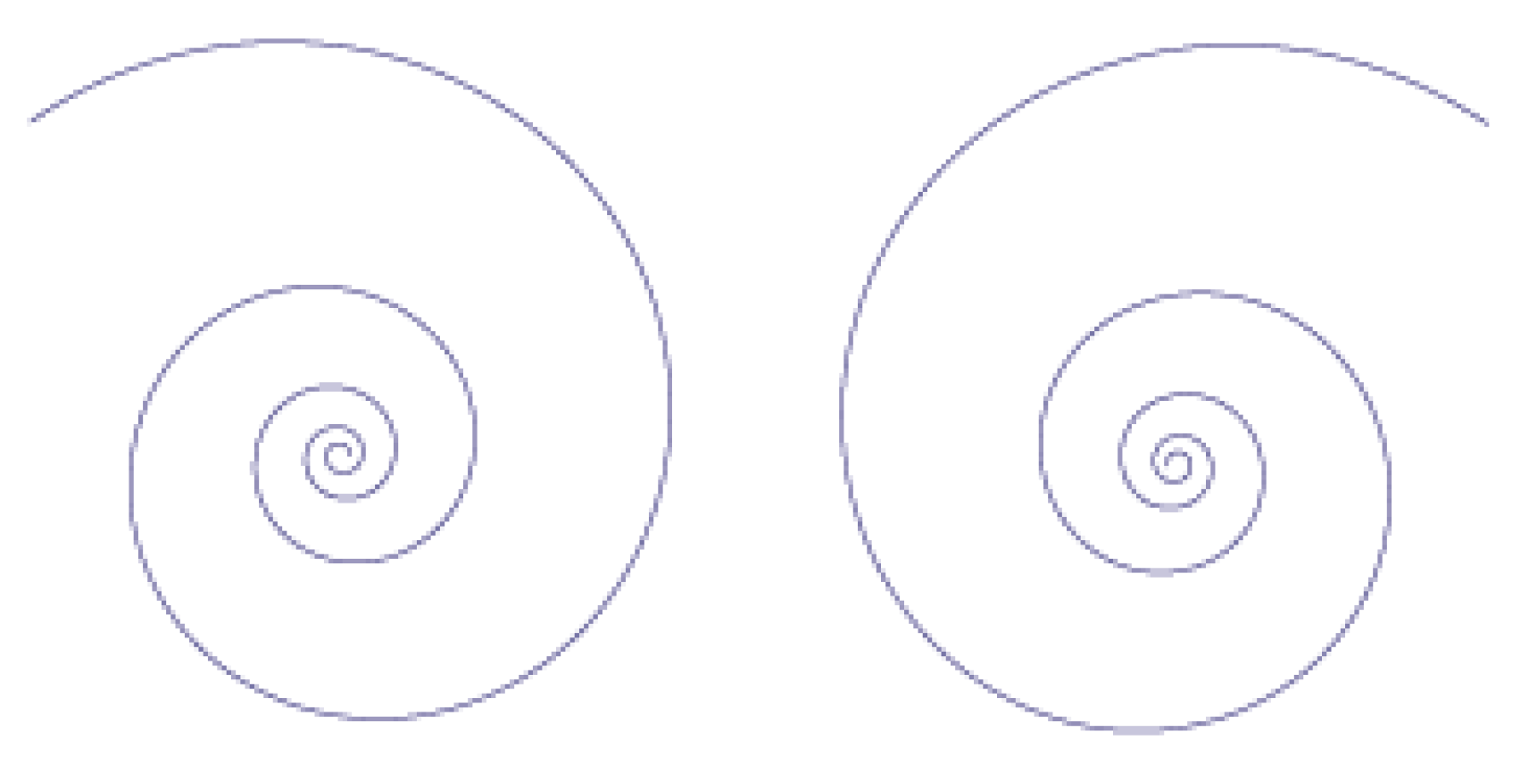
Let me start with the logarithmic spiral (
Figure 1). Its representation in polar coordinates
is [
27,
28]:
with arbitrary real constants
and
d and
. Equation (
32) is represented by the straight line of slope
d in a log-log plot with abscissa
:
Figure 1.
The anti-clockwise and the clockwise logarithmic spiral.
Figure 1.
The anti-clockwise and the clockwise logarithmic spiral.
The self-similarity property is represented by the constancy of the angular coefficient
. Rescaling
affects
by the power
. The parametric equations of the spiral are:
The point
on the spiral in the complex
z-plane is fully specified once the the sign of
is assigned. The completeness of the (hyperbolic) basis
requires that the points
and
need both to be considered. Opposite signs for the imaginary exponent
also have been considered for convenience. By using the parametrization
,
and
can be shown to solve the equations (“dot" denotes derivative with respect to
t)
respectively, provided that
up to an arbitrary additive constant;
m,
γ and
κ are positive real constants. Thus the logarithmic spirals are described by
and
solutions of Equations (36) and (37) and the parameter
t can be interpreted as the time parameter. The notations
and
, with
, are the same as in
Section 3. Note that by putting
and
, Equations (36) and (37) reduce to Equations (16) and (17) (namely they provide an equivalent representation of Equations (5) and (6)). Observe that
at
. At
,
,
, with integer
... We thus see that the continuous character of Equations (34) and (35) (which is reflected in the continuous time evolution according to Equation (
38)) also includes as a subset, due to the T integer multiplicity, the discrete group transformation
. This suggests to us that the isomorphism we refer to appears as a homomorphism. Such an occurrence is indeed implicit in the very same structure of Equations (34) and (35) describing the logarithmic spiral. A similar situation occurs in the case of the Koch curve and other fractals considered below. We plan to present a deeper analysis of this point in a future paper. The spiral “angular velocity” is
. Our discussion also includes the golden spiral and its relation with Fibonacci progression (see the
Appendix).
By proceeding in a similar way as done in previous Sections, the Lagrangian, the Hamiltonian Equations (25) and (26) and also the other formulas for the evolution operator, the ground state, etc., Equations (28)–(31) are obtained for the spiral when working in the proper QFT frame. The breakdown of time-reversal symmetry is again associated with the choice of a privileged direction in time evolution and the entropy operator S may be defined. The left-handed chirality spiral (direct spiral, ) is the time-reversed, but distinct, image of the right-handed chirality spiral (indirect spiral, ).
The Hamiltonian
H is actually the
fractal free energy for the coherent boson condensation process out of which the fractal is formed.
can be identified with the “internal energy”
U and
with the entropy
S. From Equation (
26) and the defining equation for the temperature
T (putting
), we have
and obtain
. Thus,
H represents the free energy
. The heat contribution in
is given by
and
. The temperature
is found to be proportional to the background zero point energy:
[
3,
22,
23,
24].
The evolution operator
, when written in terms of the
a and
b operators (see
Section 4), becomes [
3,
16,
17,
18]
and it is recognized to be the two mode squeezing generator with squeezing parameter
. The
generalized coherent state (29) is thus a squeezed state.
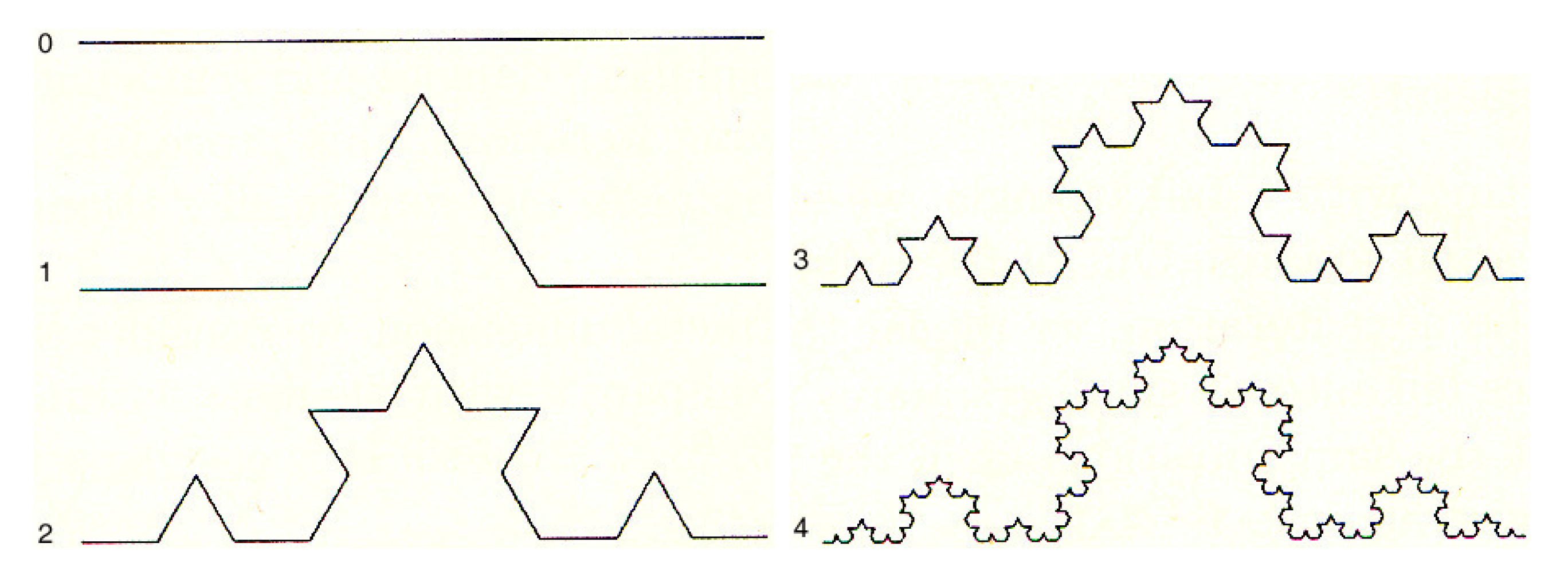
Consider now the examples of the Koch curve [
26,
27]. Let
for the initial stage
(see
Figure 2) [
5]. The
n-th step or stage is denoted by
, with
and
[
6,
7]. One has
which gives the self-similarity, or fractal dimension [
27]
. It is important to stress that self-similarity is properly defined only in the
limit. Put
and write the self-similarity equation for
in polar coordinates as
, which is similar to Equation (
32) (or as
which is similar to Equation (
33)). One can proceed then as in the case of the logarithmic spiral, the parametric equations for the fractal in the
z-plane can be written, and so on to obtain the fractal Hamiltonian and free energy. The exponential operator in the evolution operator
is
where
and
denote the doubled degrees of freedom and
,
.
In conclusion, the relation between the self-similarity of logarithmic spiral and the Koch curve and the SU(1,1) generalized coherent state is thus established.
It is also interesting to consider the relation of the Koch curve with Glauber coherent states. Indeed, apart the normalization factor
, the functions
are recognized to be the restriction to real
of the functions
which form a basis in the space
of the entire analytic functions. Therefore, the fractal properties can be studied in
, by restricting, at the end, the results to real
,
[
6,
7]. The relation with coherent states is established by realizing that
provides the Fock-Bargmann representation of the Weyl–Heisenberg algebra [
14], namely, the frame where (Glauber) coherent states are described. Define
and apply
to the coherent state
,
; one finds the so-called
q-deformed coherent state
Figure 2.
The first five stages of Koch curve.
Figure 2.
The first five stages of Koch curve.
Here
, with
a the annihilator operator. Apply
to
and restrict then to real
:
which gives the
n-th iteration stage of the fractal. The operator
acts as a “magnifying” lens [
6,
7,
26]. In conclusion, the one-to-one correspondence is established between the fractal
n-th stage of iteration,
, and the
n-th term in the
q-deformed coherent state Equation (
43).
is a squeezed coherent state [
16,
17,
18,
29] with squeezing parameter
and
, called
the fractal operator [
6,
7], is the squeezing operator in
. The squeezing transformation of the coherent state therefore describes the self-similarity properties of the Koch curve (and other fractals).
Let me close this Section with a comment on noncommutative geometry arising as an effect of dissipation [
30]. In the
plane use the notation
and
, so that
denote the momenta and
the forward in time and backward in time velocities:
The relation between dissipation and noncommutative geometry in the plane is thus obtained since the canonical set of conjugate position coordinates
can be then defined by putting
, with
The area enclosed in the two paths and is proportional to the quantum dissipative interference phase in the noncommutative plane, provided .
On the other hand, the algebraic structure of the doubling of the degrees of freedom introduced above in order to close the system is a noncommutative one. The algebra is indeed duplicated by the map
, which is the Hopf coproduct map
. Convenient combinations of the deformed coproducts in the
q-deformed Hopf algebra, which are noncommutative [
3,
16,
17,
18,
31,
32], produce the Bogoliubov transformations of “angle”
and the
q-deformation parameter controls the coherent condensate of the state
. This provides the physical meaning of the deformed Hopf algebraic structure and of the non-trivial topology of paths in the phase space [
31,
33].
6. Conclusions
In this paper I have shown that, in space-time regions where the magnetic field may be approximated to be constant and the electric field is derivable from a harmonic potential, an isomorphism exists between (classical and quantum) electrodynamics and the set of damped and amplified oscillators representing a prototype of a dissipative system and the environment or bath in which it is embedded, respectively. It is known [
5,
6,
7,
8], on the other hand, that such a system of oscillators is isomorph to fractal self-similar structures. On the basis of these isomorphisms a link therefore is established between electrodynamics, dissipation and self-similarity. Moreover, the ground state of the oscillator system turns out to be a generalized
q-deformed (or squeezed)
coherent state. Coherent states thus appear to play a crucial role in our discussion. I also observe that quantum dissipation implies in a natural way noncommutative geometry in the plane and the notion of dissipative interference phase [
6,
7,
8]. A rich, many-facet scenario thus emerges which certainly deserves further study. For example, it is interesting to observe that recently quantum electrodynamics has been shown [
25] to be naturally described by
rather than Weyl-Heisenberg algebra, which seems to agree with the general picture of the present paper establishing the relation between the
system of damped/amplified oscillators and electrodynamics.
One more aspect which is related with the discussion here presented concerns with the description of fractal-like structures with self-similarity properties in terms of non-homogeneous Bose condensation. Indeed, in the present scheme they appear to be generated by coherent
quantum condensation processes at the microscopic level, similar to “extended objects” or
macroscopic quantum systems [
1,
2,
3,
4], such as crystals, ferromagnets and like systems in condensed matter physics characterized by ordered patterns. The macroscopic appearances (
forms) of the fractals seems to emerge out of a process of
morphogenesis as the macroscopic manifestation of the underlying dissipative, coherent quantum dynamics at the elementary level. An integrated vision of Nature resting, in its essence, on the paradigm of coherence and dissipation thus emerges. Even the sector of high energy physics, with the recent discovery of the Higgs boson and the coherent condensate structure of the vacuum, belongs to such a picture. Nature appears to be modulated by coherence, rather than being hierarchically layered in isolated compartments, in multi-coded collections of isolated systems and phenomena [
5,
34]. One might express this by saying that the dynamics of coherence is the primordial origin of
codes. In this way codes are promoted from the (syntactic) level of pure information (à la Shannon) to the (semantic) level of
meanings, expressions of coherent dynamical processes.
Let me close with a further comment concerning living matter physics. That coherence comes before the code seems to be supported also by the DNA duplication processes currently done in biological laboratories. In these polymerase chain reaction (PCR) processes, samples of water solutions containing the parent DNA (the template), primers, nucleotides and enzymes are submitted to sequences of thermal cycles. The DNA template transfers to the water in which it is embedded, by means of the emission of its em signal, the coherent structure of which its code is the expression. It turns out indeed that such an em signal has fractal-like self-similar structure and therefore, according to the theorem above discussed, it is expression of coherent dynamics. The duplicated DNA (reproducing the specific sequence of nucleotides of the parent DNA macromolecule),
i.e., the genetic DNA code, is “re-constructed” as the dynamical output of the interaction of the coherent em signal with the water medium, and, through this, with the primers and nucleotides in the solution. In recent experiments [
35] it has been possible to record the em signal emitted by aqueous solutions of DNA of viruses and bacteria and it has been shown that they have fractal-like self-similar structure. These signals have been used to irradiate (to “signalize”) water. Then the original (parent) DNA has been reconstructed by use of usual PCR protocols, provided that primers and nucleotides, but not the template DNA, are added in the water solution. The occurrence of such a phenomenon also suggests that deformation (squeezing) of the signal coherence may induce dynamical epigenetic modifications, which may then signal the appearance of
new meanings associated to deformed coherent signals. The DNA genetic code appears in conclusion to be the output of the coherent dynamics. In this way, it is subtracted from its purely phenomenological characterization, which is sometimes at the origin of dogmatic or even miraculous beliefs. In this view, DNA appears to be the vehicle through which the laws of form express themselves in living systems and coherence and its deformations propagate through duplication and multiplication processes.


