A Systems Engineering Methodology for Designing and Planning the Built Environment—Results from the Urban Research Laboratory Nuremberg and Their Integration in Education

Abstract

Sustainable urban development requires a long-term sector-integrative approach. This paper proposes a method of system analysis and partial simulation for urban structures for this purpose. It couples a discussion-based holistic approach for systems analysis and modelling of urban structures with quantitative modelling and simulation of partial scenarios that serve to examine specific questions regarding the long-term development of urban structures. In the first part, the application in the City Lab Nuremberg West, a multidisciplinary urban research laboratory, serves to develop the methodology and its illustration. The main objective is to examine the transition of the existing underperforming quarter to a sustainable and livable urban environment. Scenario-based experiments with respect to development paths determine robustness and risks of different configurations. The second part of the paper describes the transfer of the methodology to education. The approach serves to teach students in the Energy-Efficient and Sustainable Building master course program an integrative way of planning a sustainable built environment. The definition of educational objectives concerning the students’ understanding and management of systemic interdependencies of sustainability help assess the use of the method in the classroom. The aim is to provide them with the competence to develop strategies for complex situations while planning a sustainable built environment.

1. Introduction: Sustainable Design and Planning in Research and Education

1.1. The Research Approach: Long-Term Urban Planning at the City Lab Nuremberg Western City

The impacts of global change are increasingly affecting cities and urban agglomerations. Economic, social, technological and ecological changes, such as climate change or the latest transformative changes to the energy policy in Germany (“Energiewende”) impose significant challenges that influence the conversion of existing neighborhoods and communities. Cities are highly complex spatial agglomerations. In order to adequately understand cities, a variety of levels and aspects have to be considered. These include urban planning, building design, infrastructure, functions, aesthetics and various others topics. In order to create a basis for an integrated view of options for the future development of Nuremberg West, we performed a fundamental analysis of the current situation. This included the interaction of different scales, disciplines and approaches. The knowledge of different working methods, levels of detail and references was crucial to create a basis for the interdisciplinary collaboration of the various disciplines and work areas, such as urban planning, landscape planning, resource consumption/energy efficiency and transport planning.

In this context, we developed a method of systems modelling that addresses the complex interdependencies and supports the development of strategic solutions for sustainable urban development. This development took place in the interdisciplinary research project City Lab Nuremberg West at the Technische Universität München and dealt with these challenges in order to establish long-term strategies for the development of a livable and sustainable future for this urban district, which has approx. 15,000 inhabitants.

The main purpose of this development is to derive a method to set up a systems model that supports decision processes in planning and designing the built environment and is tailored specifically for this purpose. This includes the derivation of the model in a discussion-based process between the disciplinary stakeholders and it describes the analysis and simulation of the systems model supporting the development of sustainable strategies in the planning context as an assisting tool. It allows the simulation of time-based transitions of the urban quarter such as those required for the Energiewende. The paper describes the methodology, its computer implementation and its transfer to education, which is outlined at the end of this section.

1.2. Importance of Long-Term Strategies

Based on the analysis and study of global trends, we developed three alternative visions, called development paths, for a plausible future aimed at the coming decades until the year 2050. Long-term strategies are crucial especially with regard to the development of key projects, sites and locations, as the short-term realization of supposedly appropriate projects on specific locations might prohibit the future viability of sustainable projects in these locations.

With regard to the realization of higher-level measures, such as the infrastructure of the city, including energy systems, individual and public transport as well as water supply and sewage systems, long-term thinking and strategic planning were crucial for the economic feasibility of these measures. In order to be able to propose and implement radical solutions in the planning process, longer periods of time are crucial for the economic feasibility of fundamental changes in the infrastructure that might be necessary to allow for the realization of sustainable concepts.

1.3. Integrated Urban Modelling in Research

The City Lab Nuremberg West places special emphasis on the ‘livable city’ as a major aspect of a sustainable urban development. It becomes apparent that many different sectors contribute to the emergence of a city worth living in, both in terms of content as well as in terms of the various administrative levels, such as the state, the city and the private level. It requires the integration of a very wide range of topics, such as economy, health, mobility, culture, identity, food supply, quality of the built environment and many other aspects.

Current research aims at sector-oriented modelling and simulation of the behavior of urban structures; Robinson [1] gives an overview of these developments. There is a history of sector-crossing systems modelling that also addresses the urban context with comprehensive general models, such as Urban Dynamics by Forrester [2] to name a prominent instance. However, large-scale approaches have often been criticized due to not being manageable and not being able to make correct predictions [3]. Nevertheless, they are still an important part of models predicting the behavior of urban systems in planning and decision-making, especially for land use and urban transport [4]. Furthermore, urban structures are seen as complex systems for which a systems approach provides the basis for current scientific examination [5,6].

In contrast to large-scale comprehensive system models that aim for a general understanding of the behavior of urban structures, our approach uses problem-specific partial models for the specific planning demand and its inherent questions. Expert discussion serves to develop the systems model. For Nuremberg West, the discussion-based system definition focused on the sectors functionality, energy and resource consumption, mobility and urban quality. In addition to the sectoral analysis as part of long-term planning and control, an integrative view is also required. The dependencies of the many individual aspects of the various sectors and disciplines lead to a complex system that must be considered for long-term urban development. To detect and investigate the dependencies of the various factors, the method of sensitivity modelling as described by Vester [7] was applied, which forms an important step of the discussion-based setup of the system model. This methodology is used to detect the influences in an expert discussion between variables and trends of various sectors, and to map their effects.

1.4. Planning-Embedded, Time-Based Simulation

Cities are dynamically evolving structures and are constantly in transition due to continuous changes in many areas, such as population, functional requirements and economic conditions. Furthermore, global and local trends influence the development of a city. Based on these trends, the three different development paths mentioned above were developed to describe three fundamentally different, yet plausible alternative development paths for the coming decades until 2050. The alternative development paths depend on the following three economic patterns: (1) economic growth (knowledge-based economy hub), (2) economic standstill (managed care) and (3) economic decline (subsistence economy). In all of these three alternative visions of the future the concept of a livable city was used as an indispensable basis for the development.

Therefore, this paper—after performing systems modelling and analysis—proposes a method of systems modelling and partial simulation that is adapted to the specific situation of long-term urban planning and development. The purpose of the time-based simulation is to gain information about the interaction of the sectors and disciplines and to learn about the time-related development of the district in a long-term perspective. This includes information about the planned and expected effects in terms of their strength and timing but also the identification of unexpected side effects and development risks.

This use of the system simulation is embedded in the planning process and acts as a tool for decision-making. Therefore, embedding a detailed, but partial system simulation model in the decision process is a central aim of the approach. The model is derived from the planning process with its discussions and feeds its results back to this process. It is a tool to answer specific questions occurring in the planning process for which the method provides quantified intersectoral support to answer them appropriately. This helps overcome the usual arbitrary and implicit decision-making without a quantitative basis that often occurs in design and planning.

The method starts by modelling the system structure through expert discussion, as proposed by Vester [7]. The key variables and interdependencies as well as the objectives and external conditions—the latter described as development paths—result from this process. The next step is the definition of partial scenarios for simulation, again in experts’ discussion. For systems modelling, this paper presents an adapted method for partial system simulation that differs from the method proposed by Vester, which is available as software by Malik [8]. The adapted method includes a continuous simulation approach in contrast to Vester’s discrete simulation method; it allows different types of interdependencies and the linkage of the system scales and interdependencies to real values. A partial simulation for Nuremberg Western City was implemented based on the adapted method. The example results of this implementation demonstrate how the systems model with its simulation can support the planning process, providing answers to questions and examining risks and potentials for long-term urban planning.

1.5. The Education Approach: Integrative System-Based Understanding and Thinking for a Sustainable Built Environment

Interaction between different sectors and planning disciplines plays an important role in the education of architects, civil engineers and environmental engineers in sustainable planning. Many design and planning curricula now include mono-disciplinary views of sustainable planning and building, such as building services and thermal energy, transport, solar architecture, water management, etc. However, the integration of these views is lacking. Normally, students do not learn to assess interactions between the sectors and to weigh up sectoral benefits while considering that investments usually are limited and embedded in economic and social structures.

This was the situation for the Master’s in Energy-Efficient and Sustainable Building course at the Technische Universität München. A lecture series in the module Sustainable Architecture, City and Landscape Planning (SACLP) provided sectoral views and included a seminar that bridges the sectoral view and introduces students to an integrative approach. Thus, the idea arose to transfer the methods of the City Lab Nuremberg West to education in this Master’s course. The main challenge of this transfer was to introduce students to systems thinking, which we deem a core competence for sustainable building. The aim of the method transfer is to identify key parameters as well as strategies for sustainable built structures in a qualitative way as well as to provide students with the ability to quantitatively model sector-crossing interdisciplinary dependencies and their effects.

2. Systems Modelling in Research—City Lab Nuremberg West

The first step of the method developed in the research project City Lab Nuremberg West is to use the methodology of sensitivity analysis developed by Frederic Vester [7] as a starting point to build up the systems model and adapt it for urban structures. This approach is very appealing, especially for those not familiar with system engineering since it is easy to understand and uses many stakeholder discussion procedures. One major adaptation for long term planning is the use of development paths, which are described in Section 2.2.

As the second step after developing the structure of the systems model using Vester’s approach, the method had to be significantly changed from a discrete event approach to a continuous dynamic simulation method. The subsection on quantitative systems modelling for partial simulation describes this continuous dynamic method. This development allowed mixed qualitative-quantitative modelling with the precision required for the challenge of a sustainable and livable urban structure as envisioned for Nuremberg Western City.

The discussion-based setup of the systems model, which is the first part of the methodology, led the team to a problem-specific partial setup of the systems model. This process took place in two systems modelling workshops and further regular project team meetings. These events defined the information in the Section 2.1, Section 2.2 and Section 2.3. The aim of the discussion process is to reach agreement among the stakeholders on the system and its parts, its description by variables and the relevant dependencies between the variables. Section 2.4 and Section 2.5 describe the implementation of simulations.

2.1. Sensitivity Analysis, Systems Modelling and the Planning Process

The first step is the analysis of interdependencies by the influence matrix. For this purpose, the expert committee defines n variables describing the state of the system and, following the method of Vester, discusses and agrees on one effect strength between all n²-n combinations in a matrix:

▼has effect on ►	V1	V2	V3	V4	Active sum
V1	-	2	1	2	5
V2	3	-	0	1	4
V3	0	1	-	2	3
V4	3	1	2	-	6
Passive sum	6	4	3	5

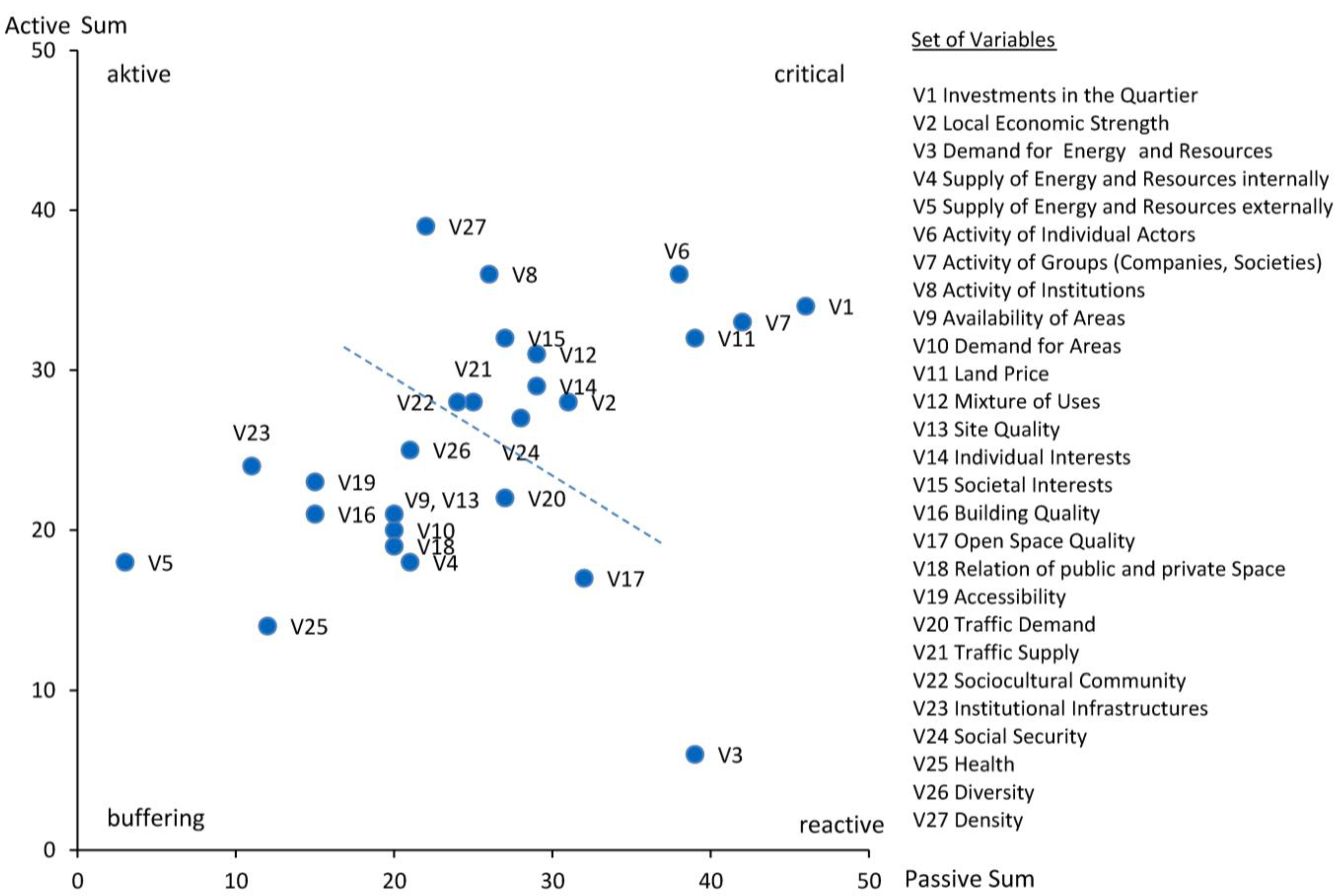
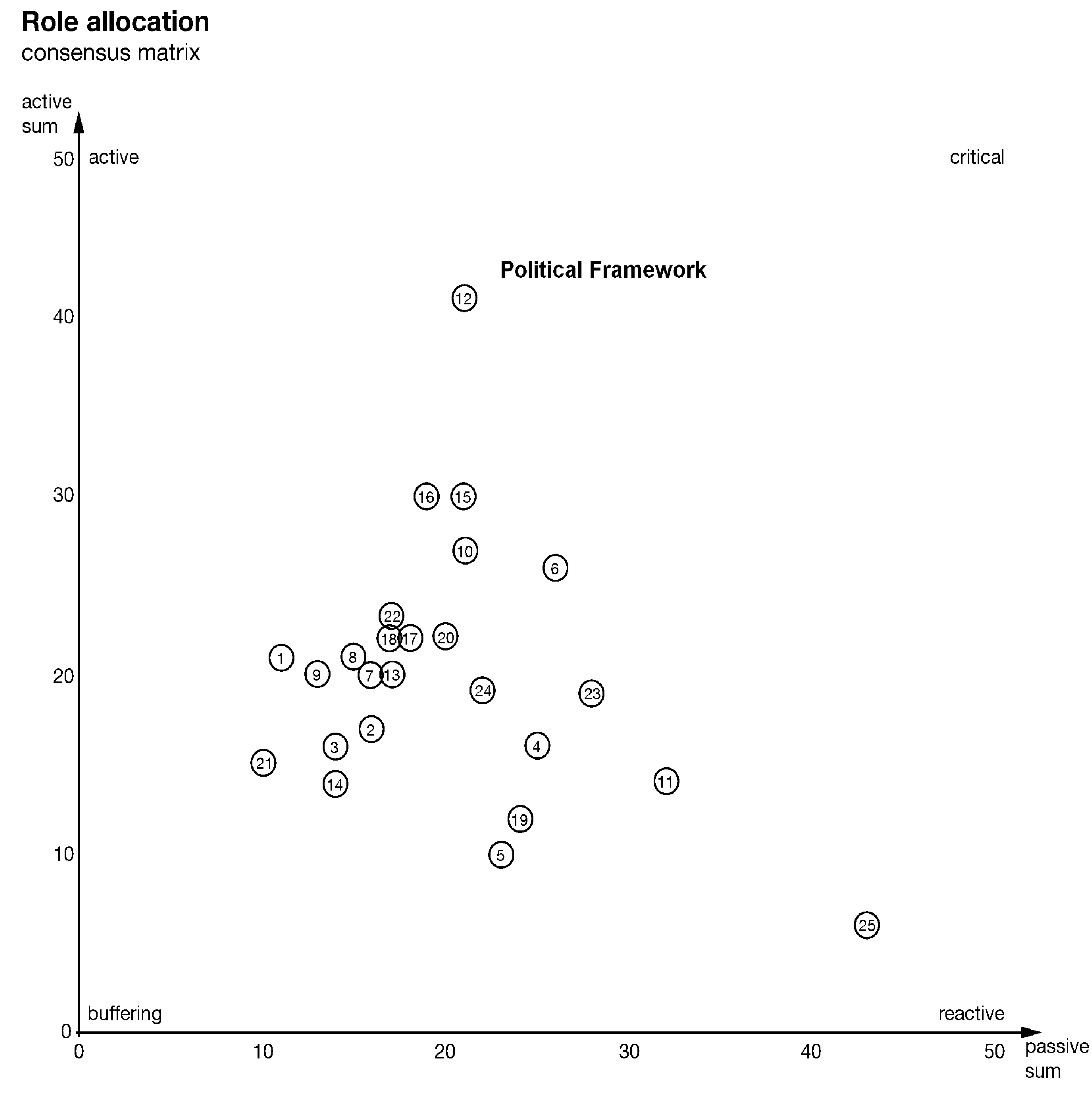
The matrix equals the methods of the design structure matrix (DSM), as proposed by Eppinger and Browning [9]. The result of this procedure, which was carried out for Nuremberg Western City in two workshops, is to define the role of the variables in the system. In detail, the active and the passive sums describe the extent to which variables influence one another. Figure 1 shows the role of the variables based on these sums.

Figure 1. Role of variables in the system.

Figure 1. Role of variables in the system.

The role of variables allows us to select variables and relevant interdependencies for building the partial system model. Active variables, such as V27 Density, V6–8 Activity of Actors, V1 Investments and V11 Land Price, or reactive variables, such as the V3 Demand of Energy and Resources, are particularly interesting for setting up the system. Variables that are both active and reactive, and therefore critical, should also be included, but handled with care. The active variables are most interesting for the control of the system and for respective measures. Critical variables also allow for effective control of the system. However, as they react strongly to other variables, their adjustment tends to cause systemic instabilities. According to these considerations, variables above the dashed line are the primary candidates for the partial simulation.

2.2. Development Paths and Scenarios

One innovation in applying systems modelling in the long-term development of urban structures is to integrate a scheme of development paths and scenarios. Development paths define varying external and internal conditions of the urban district, which are mainly influenced by processes, decisions and states outside the district. They are a new feature of long-term urban planning that originated from the work by the Nuremberg Western City team [10].

Scenarios are subordinate to development paths and describe possible variations within them in order to examine risks and potentials. Scenarios form the basis for examinations in the partial simulation; they vary whereas the development paths represent fixed basic conditions for these examinations.

In the Nuremberg Western City project, the alternative development paths depend on the following three alternative economic development patterns: economic growth, economic standstill and economic decline. These three alternatives were named “knowledge economy hub”, “managed care”, and “subsistence economy”. In all of these alternative visions, the concept of a livable city was taken as an indispensable basis for development.

Knowledge economy hub: The first path assumes that Nuremberg Western City evolves into a well-performing knowledge economy site. High economic activity takes place and leads to comprehensive investments.

Managed care: The second path describes a quarter mainly characterized by residential use that takes on a service role for other districts.

Subsistence economy: The third path is based on the assumption of widespread economic decline and the subsequent creation of an alternative circulation economy that features small local value-adding activities.

2.3. Quantitative Systems Modelling for Partial Simulation

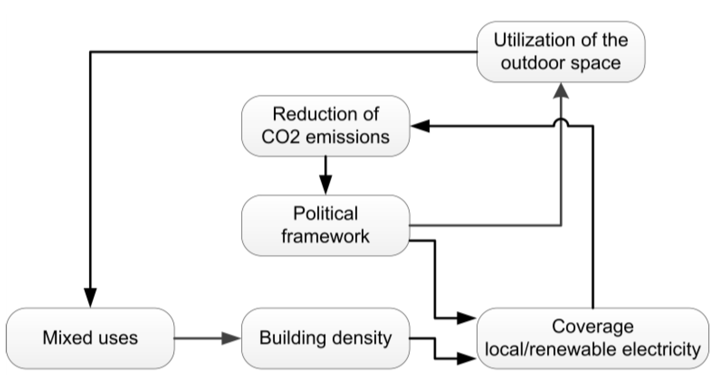
After identifying the key variables for the three paths, the next step is to select variables for the effect structures and thus for the partial simulation model. The effect structure compiles all relevant dependencies in a graphic structure with their direction and sign but without magnitude, as shown in Figure 2. The occurrence and importance of qualitative as well as quantitative variables requires an intermediating approach. For this purpose, the approach uses substitute scales that normalize all variables to a range between 0 and 1 (for details see Geyer et al. [11]). The detailed definition of the scales of the real values and of the mapping to the substitute scale is required to determine the interdependencies, as described later in this section. Table 1 shows these definitions for the case Nuremberg Western City. Except in one case, a simple linear mapping is used for the scales. Only urban density is mapped using logarithmic transformation; as a result, except for table-defined dependencies, the interdependencies between this variable and the other variable are linear.

To model the interdependencies in detail for the simulation the approach proposed in this paper, in contrast to Vester [7], mainly uses a dynamic linear influence model including three types of interdependencies:

I. Direct or static dependencies provide a factor influence on a variable. In case of a variable v₁ influencing a second variable v₂, the following operation describes the influence with the influence factor a₂₁ and the neutral point b₂₁:

(1)

II. The first type of dynamic links provides an integrating interdependency:

(2)

III. The second type of dynamic dependencies uses derivation:

(3)

In some cases, the simple factor relation defined by a₂₁ was replaced by more sophisticated functions described by tables or diagrams.

To determine realistic data for the factor a and the neutral point b per interdependency, three different strategies are applied. First, best quality systemic dependencies derive from simulations specifically made for the quarter under consideration. As part of the Nuremberg Western City project, results from a stochastic simulation of energy efficiency measures as described in [12] were modelled as interdependency and included for investments in buildings and building energy consumption. Secondly, empirical studies on specific dependencies in other urban contexts are the next source of interdependencies in the model. For example, results from Kenworthy and Laube [13] serve to model the interdependency of transport demand and density or data from Fischer [14] for the influence of density and mixture of use on social security. Thirdly, the evaluation of statistical data is a source to determine interdependencies, such as the influence of density on land value, which was determined by regression analysis of the standard land value and the number of inhabitants and workplaces in the area of Nuremberg [15].

Figure 2. Effect structure modelled for Nuremberg Western City.

Figure 2. Effect structure modelled for Nuremberg Western City.

Table 1. Definition of the variables used for the partial simulation.

Variable	Description	Scale
V1 Investments	Total investments per inhabitant/workplace	Quantitative: 500…10,000 EUR per cap. and yr.
V3a Energy demand	Energy demand in the district	Quantitative: 5,000…75,000 kWh per cap. and yr.
V5a External energy supply	The energy price describes the external energy supply	Quantitative: 50…200% (comp. to 2012)
V6–8 Actor activity	Activity of individuals, groups (companies/societies) and institutions	Qualitative: 0% (passive) … 100% (active)
V12 Mixture of use	Mixture of use describes the distance to most important uses in the city	Qualitative: 0% (monoculture) … 100% (mixed use)
V14 Individual interests	Describes the realization of individual interests (e.g., employment)	Qualitative: 0% (restricted) … 100% (realized)
V15a Reduction of CO2 emissions	Common interest of reducing CO2 emissions	Quantitative: 15 … 0 t CO2-eq. per cap. and yr.
V16 Building quality	Technical and spatial quality, construction cost as simplified measure	Quantitative: Residential: 750 … 1,500 € per m2 gross areaOffice: 1,000 … 2,000 € per m2 gross area
V19 Accessibility	Average travel times per journey	Quantitative: 20 … 60 min
V20a Transport sustainability	Share held by ecomobility	Qualitative:
		Scale	Cycle	Public transport	Cars
		100%	0%	40%	20%
		0%	20%	10%	70%
V20b Transport demand	Weekly travelled distance per person.	Quantitative: 200 … 100 km per person and week
V22 Sociocultural community	Integration of different groups of users and inhabitants	Qualitative: 0% (segregated) … 100% (integrated)
V24/25 Social security/health	Social security and health of the users	Qualitative: 0% (low) … 100% (high)
V27 Density	Inhabitants and users per area	Quantitative: 15 … 150 persons per ha (logarithmic scale)

Table 1. Definition of the variables used for the partial simulation.

Variable	Description	Scale
V1 Investments	Total investments per inhabitant/workplace	Quantitative: 500…10,000 EUR per cap. and yr.
V3a Energy demand	Energy demand in the district	Quantitative: 5,000…75,000 kWh per cap. and yr.
V5a External energy supply	The energy price describes the external energy supply	Quantitative: 50…200% (comp. to 2012)
V6–8 Actor activity	Activity of individuals, groups (companies/societies) and institutions	Qualitative: 0% (passive) … 100% (active)
V12 Mixture of use	Mixture of use describes the distance to most important uses in the city	Qualitative: 0% (monoculture) … 100% (mixed use)
V14 Individual interests	Describes the realization of individual interests (e.g., employment)	Qualitative: 0% (restricted) … 100% (realized)
V15a Reduction of CO2 emissions	Common interest of reducing CO2 emissions	Quantitative: 15 … 0 t CO2-eq. per cap. and yr.
V16 Building quality	Technical and spatial quality, construction cost as simplified measure	Quantitative: Residential: 750 … 1,500 € per m2 gross areaOffice: 1,000 … 2,000 € per m2 gross area
V19 Accessibility	Average travel times per journey	Quantitative: 20 … 60 min
V20a Transport sustainability	Share held by ecomobility	Qualitative:
		Scale	Cycle	Public transport	Cars
		100%	0%	40%	20%
		0%	20%	10%	70%
V20b Transport demand	Weekly travelled distance per person.	Quantitative: 200 … 100 km per person and week
V22 Sociocultural community	Integration of different groups of users and inhabitants	Qualitative: 0% (segregated) … 100% (integrated)
V24/25 Social security/health	Social security and health of the users	Qualitative: 0% (low) … 100% (high)
V27 Density	Inhabitants and users per area	Quantitative: 15 … 150 persons per ha (logarithmic scale)

These strategies lead to information for all interdependencies included in the partial effect structure selected for simulation implementation. Figure 2 shows the effect structure and its interdependency values. This structure has a main focus on built structures and transport. Furthermore, it considers energy, investments, and social aspects. The interpretation of the simulation results will take this partial character into account.

2.4. Implementation

Besides the development of methodology, one aim of the research approach is to set up a systems modelling environment for buildings and urban structures. Therefore, experiments include testing of modelling and simulation environments using the visual programming approach. The structure of objects in this modelling environment was object oriented so that not only the environment with its graphic user interface and interactive procedures is developed, but also the elements of which the model is composed.

The visual user interface aims at representing a block diagram with objects as boxes and interdependencies as connectors in between, which is very close to an internal block diagram (ibd) of the Systems Modelling Language (SysML, [16]). The SysML is very suitable for the purpose for two reasons: First, it is a standardized way of modelling systems and representing systemic interdependencies; second, it is based on the software engineering Unified Modelling Language (UML), which eases later implementation. Another aim of the visual user interface was not only to represent the current state of the variables and their links, but also to allow for rapid, flexible and adaptive modelling and simulation of different configurations. Moreover, a powerful equation solver was required. After developing the structure as SysML diagrams, the Simulink environment within MatLab was chosen as an experimental platform because of its interactive user interface with a solver. It represents the instances of variables and the information flows between them visually, allowing interactive editing. At the same time Simulink provides access to powerful MatLab solvers allowing complex dynamic calculations.

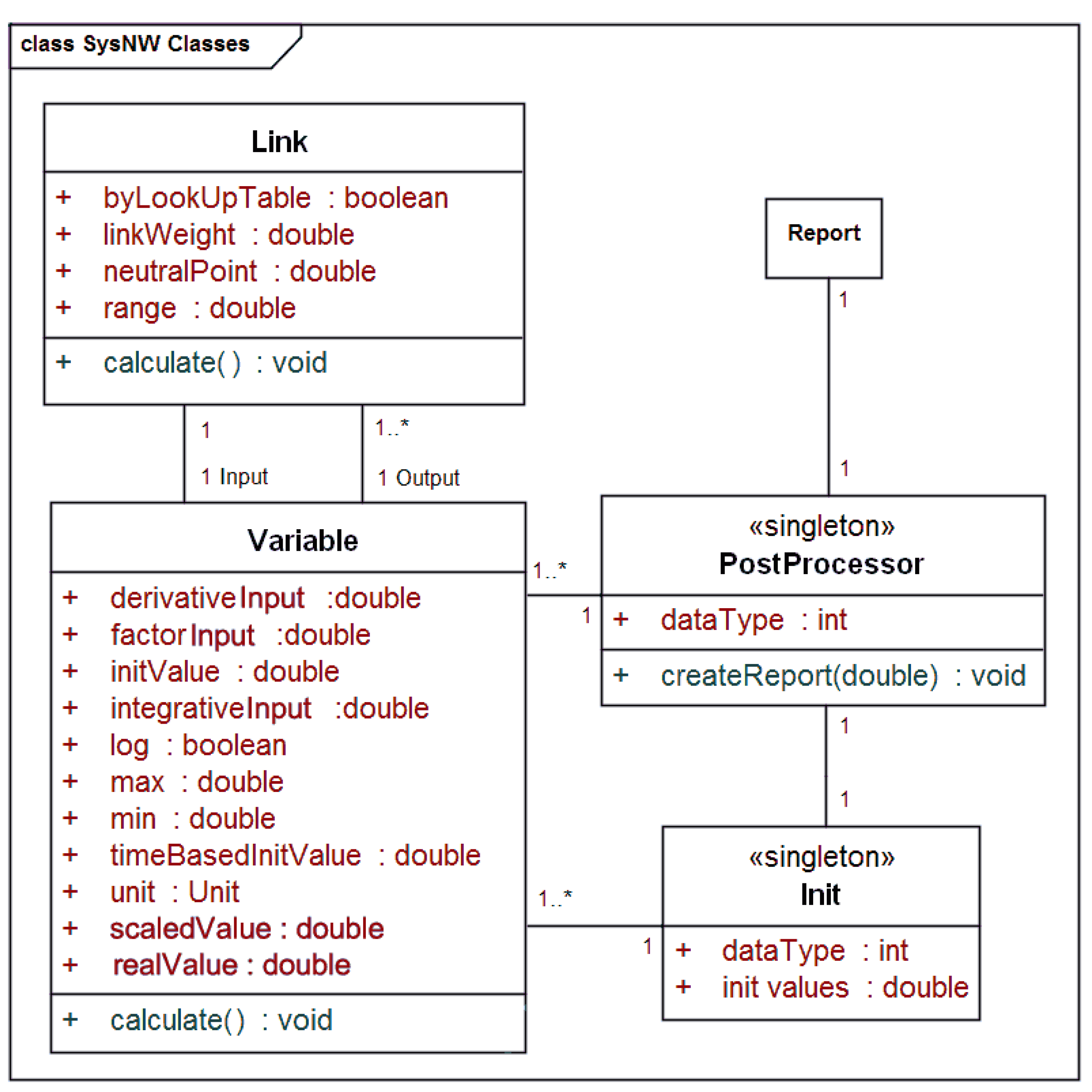
The SysML model was implemented based on five classes (Class diagram, Figure 3). Each model variable is represented by an instance of the Variable class. The method “calculate” implements the update calculation of the variables; it gathers the values “factorInput”, “integrationInput” and “derivationInput” according to the three dependency types described in Section 2.3 and generates the results “scaledValue” and “realValue”. The class supports time-dependent or constant initial values (“initValue”/“timeBasedInitValue”). After calculation, the output value is available for other variables by using one or multiple instances of the Link class. The link implements linear scaling of interdependencies as shown in Equations (1–3) with the parameters a and b. Therefore, it requires the attributes link weight w, neutral point b, range a and a switch for using a lookup table instead of linear dependency definition. The output values of a variable can also be connected to the postprocessor, which will create and render a report. The class ‘Init’ hosts the time-dependent development of the predefined variables and some configuration settings for the postprocessor.

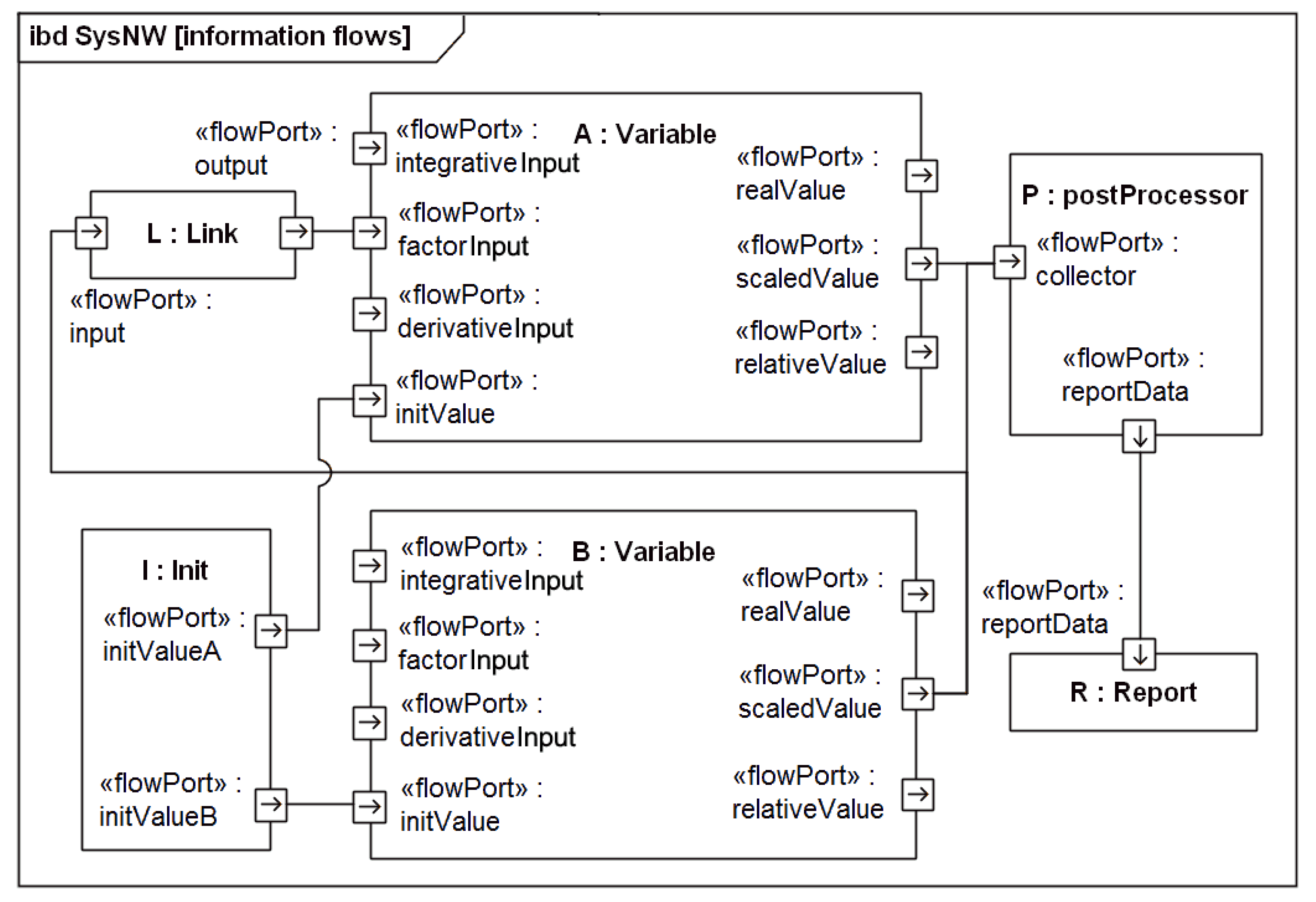
The implementation of the framework in Simulink sets up a systemic information flow model as shown exemplarily in Figure 4. The model represents system variables as instances of the Variable class (Variable A and Variable B). Each of them has one input port for time-dependent init values and three input ports for factor, integrative and derivative interdependencies. Both variables receive time-dependent initial values from the init instance. There are three output signals available: real, scaled and relative value. The real value contains the absolute value according to the variables unit; the scaled value contains the substitute scale value that is used for linking variables (for scales see Table 1). The relative value contains the percent change from the initial value for the report. An instance of the link class is required to create interdependency between two variables (Figure 4 Link). Its input port is connected to the scaled value output of variable B and its output signal is linked to the factor input of variable A. As a result, the scaled value of variable B has a static influence on variable A with the properties defined by the link’s attributes. The scaled values of both variables are connected to the instance “PostProcessor”, which creates a report describing the time-related development of the variables in the system.

Figure 3. Variable and link classes.

Figure 3. Variable and link classes.

Figure 4. Internal block diagram (SysML) of an example model setup with information flows.

Figure 4. Internal block diagram (SysML) of an example model setup with information flows.

The variables are created and configured using Simulink’s visual programming environment. Figure 5 shows an example of variable V1 Investments, with a time-dependent initial Value (Val) and a factor influence from variable V6–8. There are no integrative influences and derivative influences are not implemented yet, because the first does not apply to the variable and the second is not present in the Nuremberg Western City model. The attribute’s values are also displayed in the variable instance, in this case, the substitute scale’s maximum is set to 10,000.00 and the minimum to 500.00, the unit is set to “EUR/(cap·yr)”. All outputs are passed on to the post processor, which collects results and provides a report. Furthermore, the scaled value is also connected to other variables. The attributes of the incoming link from V6–8 are also displayed in the instance representation in Simulink. Its range a is set to 0.40, the neutral point b is 0.20 and the link weight w is 1.00. The variable’s attributes can also be changed by double-clicking the instance. If there is more than one link to one variable the signals are summarized first in order to merge them into one signal. Circular links are supported by the Simulink solver engine; in Figure 3, for example, variable A could be linked back to variable B leading to a mutual interdependency with complex systemic effects that represents control circuits as they are in the real world.

Figure 5. Variable 1 “Investments”, its time-dependent initial Value (Val) and its Link from V6–8 “User Activity” in the Simulink implementation.

Figure 5. Variable 1 “Investments”, its time-dependent initial Value (Val) and its Link from V6–8 “User Activity” in the Simulink implementation.

2.5. Simulation Results and Interpretation

This section presents one selected scenario and its simulation results for the development path “knowledge economy hub” conducted for Nuremberg Western City. The aim is to illustrate the information available using time-based partial system simulation and its interpretation. The path “knowledge economy hub” describes the trend of high economic activity based on knowledge-intensive and creative services. Bundling all economic activities of this kind and the respective investments from Nuremberg to this district is a prerequisite for this path, serving to achieve the required high investments (V1) as well as medium-to-high activity of the users (V6–8). A slight increase of the density (V27) in terms of urban redensification provides further support for this configuration.

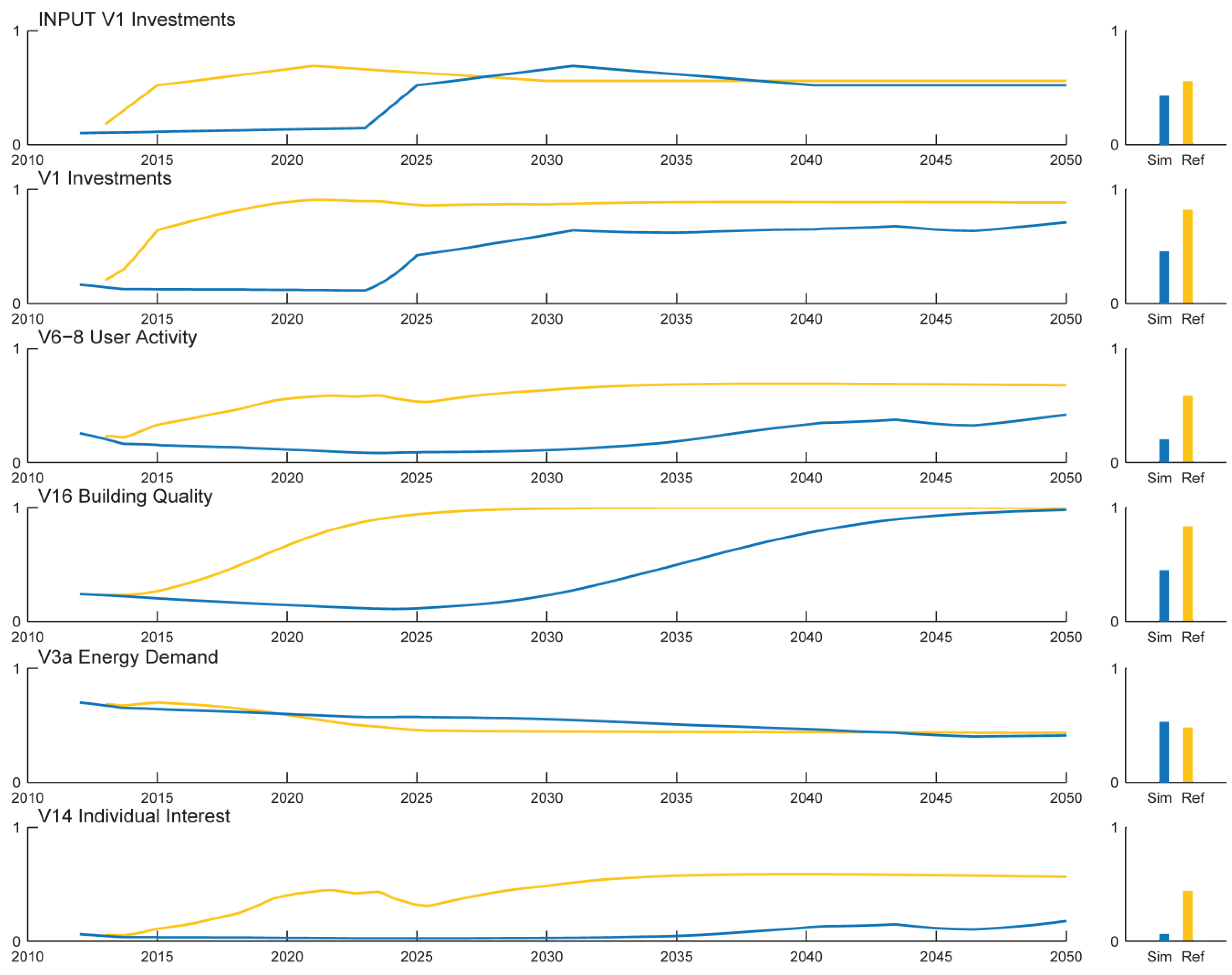
For each path, experiments using different scenarios were carried out to determine its behavior under several circumstances. Figure 6 shows one experiment with the baseline results (orange line) of the partial simulation made for this path together with one scenario (blue line). The purpose of this experiment was to examine what effect a ten-year delay in investments has on the development of the district. This is a crucial question for city administration and planners as it determines how quickly they have to act to realize the development path if they decide in favor of it.

Figure 6. Results from the partial system simulation for Nuremberg Western City.

Figure 6. Results from the partial system simulation for Nuremberg Western City.

The results of the simulation (Figure 6) clearly show the risk related to this development path. Indeed, the investments (V1) and the activity of actors (V6–8) in the delay scenario reach a similarly medium-high level as in the baseline scenario. However, user activity in the first half drops to a low level leading to strong negative side-effects such as high unemployment rates and economic decay. Furthermore, the investments delay leads to deterioration of the building stock. Nevertheless, the demand for energy (V3a) is similar in both scenarios because the reduced transport demand caused by less user activity compensates for the higher energy demand of buildings due to their bad condition. However, due to the poor circumstances of the district, such as a high unemployment rate and an unlivable environment, personal contentment (V14) is very poor in the scenario with delayed investments. This illustrates that different urban developments with equal energy consumption can have very distinct qualities in terms of their livability. Finally, the described decline of the quarter increases the risk that investments will not be made at all with the delay of ten years; as a consequence of the poor district condition investors may choose another district.

The example experiment shows that if, given appropriate conditions in the near future, the city administration decides to realize the scenario “knowledge economy hub” they must ensure that they reach the necessary level of investments within a short time. Otherwise, they risk a further significant decline of the district. The district will not have far higher energy demand but they would endanger the livability of the district (shown by low realized personal interest, V14). This in turn has a negative effect on further investments, which puts the entire development path at risk of failure, leading to a poor-condition district (as shown by the blue curves in Figure 6). In summary, this reveals the urgency for action for this path—a characteristic that significantly differs from other paths.

This simulation and interpretation of the results is just an example of how to use the method and the model in the planning context to make planning decisions or to assess actions. Further effects on other variables, further experiments and further results for other paths will be shown in [12].

2.6. Discussion

The method developed enables the identification of key system interactions and driving variables. This provides a sound foundation for partial system simulation and systemic interpretation. The first step of the overall approach is the superordinate identification and definition of the system structure including a sensitivity analysis via expert discussion. The second step is selective analysis of relevant interactions including detailed analysis and the simulation. The experts’ interpretation is an important step for the simulation to check the results for plausibility and to draw strategic conclusions. In this interpretation it is important that the simulation is not intended to exactly and absolutely predict the system state for a given moment in time. Instead it aims to observe the relative effects and interaction over the course of time. This both enables us to understand transitions, since it is a major requirement for the energy transition and the long-term urban planning situation in Nuremberg Western City and the experiments also allow us to examine the robustness of the system and identify risks and opportunities in these transitions. This enables us to carefully select development paths and to provide measures for the success of the selected development path.

3. Teaching Urban Systems Modelling—The Sustainable Architecture, City and Landscape Planning (SACLP) Course

3.1. Goals and Structure of the Seminar

The seminar Sustainable Architecture, City and Landscape Planning (SACLP), is part of the Master of Energy-Efficient and Sustainable Building [17] course at the Technische Universität München (TUM). The students, who come from different backgrounds with Bachelor’s degrees in either architecture or civil or environmental engineering, work together in interdisciplinary groups. The seminar is accompanied by a SACLP lecture series, in which professors from different areas of expertise offer students insight into their respective areas of sustainable design, planning and building. The seminar has the function of integrating the separate perspectives.

This situation gave rise to the transfer of methods of systems modelling and analysis to education. The method is applied to concrete cases of sustainable building in accordance with Vester’s Sensitivity Model. It is used to interpret cross-disciplinary relationships. For this purpose, the methodology developed in the City Lab Nuremberg West research project was adapted for use in the classroom. This transfer has taken place since the 2012/2013 winter term and the structure of the seminar is still under development. The following description represents the state of development at the end of the 2012/2013 winter term. Further developments of the seminar currently underway in the 2013/2014 winter term are outlined in the discussion in Section 3.5.

The seminar teaches students to analyze the complex relationships between different areas, sectors and disciplines, to determine the performance of a sustainable city and how to develop strategies to improve performance. The students are supposed to use an actual designing and planning case to analyze the impact of decisions in terms of sustainability and to quantify their general effect and interaction. Table 2 compiles the teaching objectives of the seminar; this is an updated version compared to the first description of the seminar in the master module made in 2012 [18].

Following the concept of Constructive Alignment [19], which highlights the importance of systematically aligning teaching and assessment to the intended teaching objectives for students, the following compilation of teaching objectives serves to verify the applied methods of systems analysis and modelling, to reflect the effect and to identify the need for further development. Implementing Constructive Alignment helps ensure that students actually acquire the previously defined skills in class and therefore represents one of the major selected concepts of TUM to assure and enhance teaching quality at university level [20].

Table 2. Compilation of the teaching objectives of the seminar “Sustainable Architecture, City and Landscape Planning” (SACLP).

No.	Description: The students are able …
1	to identify the discipline/sector-crossing interdependencies and the systemic boundary (Tax 1, 2, 3) 1
2	to structure the dependencies of sustainable building for a specific case and to identify the lever in the system (Tax 4) 1
3	to determine qualitative and quantitative systemic interdependencies (Tax 4, 5) 1
4	to focus on a specific issue in sustainable building and to develop a solution strategy by means of system modelling (Tax 5, 6) 1

¹ The “Tax” identifier shows the assessment of the cognitive level according to Anderson and Krathwohl [21].

Table 2. Compilation of the teaching objectives of the seminar “Sustainable Architecture, City and Landscape Planning” (SACLP).

No.	Description: The students are able …
1	to identify the discipline/sector-crossing interdependencies and the systemic boundary (Tax 1, 2, 3) 1
2	to structure the dependencies of sustainable building for a specific case and to identify the lever in the system (Tax 4) 1
3	to determine qualitative and quantitative systemic interdependencies (Tax 4, 5) 1
4	to focus on a specific issue in sustainable building and to develop a solution strategy by means of system modelling (Tax 5, 6) 1

¹ The “Tax” identifier shows the assessment of the cognitive level according to Anderson and Krathwohl [21].

Figure 7. Concept of the seminar.

Figure 7. Concept of the seminar.

The seminar is divided into three overlapping phases, as shown in Figure 7. In the first phase, students are introduced to the methodology and the specific project through lectures. Alongside this, the students acquire the necessary background knowledge by carrying out independent literature research. In the second phase, the system is structured and analyzed in teacher-guided discussions among students with the help of the influence matrix. In the final phase, the interdisciplinary student groups select partial scenarios (see Figure 10 in Section 3.4) from the overall model, simulate these, and interpret their results.

3.2. Development of the System Structure

In the 2012/2013 winter semester, system relationships were examined using two examples of urban structures. The first example, the Munich quarter of Gärtnerplatz in the Isarvorstadt district is a dense downtown area. The second example was the garden city Gräfelfing in the county of Munich, a sprawling suburban quarter. Using the two examples, CO₂ emissions and CO₂ reduction potential were examined across all parts of life in dense and sprawling urban regions. The main aim the students were asked to work on was recognition of the principal controlling variables for the reduction of CO₂ emissions in the system of the urban structure. The software Malik Sensitivity Model Prof. Vester^® [9] was used in the seminar to ease system analysis and simulation.

Figure 8. First sketch of the system description.

Figure 8. First sketch of the system description.

In the first phase, an introduction provides an overview of the methods and the students begin to develop the basis for system analysis, which investigates sector topics, elaborates the basic scheme of the system and defines performance criteria. Unlike the methodology developed by Vester, in order to achieve rapid understanding of the approach in one semester, an initial system description was provided as a basis for further discussions, as seen in Figure 8. The given topics also served as a template for systematic literature review in the first phase. The criteria catalog Neubau Stadtquartiere (Development of Urban Districts) by the German Society for Sustainable Building (DGNB) [22] was used as a reference for the system description and the objectives of sustainability in particular. To achieve a manageable system, the initial system description was constantly aggregated step-by-step and kept with less than 30 variables.

3.3. Analyzing the System

In Phase 2 of the seminar, the students learn to analyze and to structure the dependencies of the city district as a system as described in Section 2.1. In order to introduce the method, each step started with a workshop. Afterwards the groups completed assigned work packages on their own. In a final discussion, all students agreed on a common result for each step. The results of phases one and two were presented by the students in the mid-term presentation. The students received complete documentation as a basis for further processing.

This phase addresses Teaching Objectives 1 and 2. The discussion process required to define the variables and complete the influence matrix refers to the knowledge from the lecture and fosters sensitivity for discipline/sector-crossing interdependencies as in Teaching Objective 1. In this discussion, the students have to argue the pros and cons of interdependencies in the system transcending all sector boundaries. In our experience, they often test different points of view that are very helpful for their holistic understanding. Furthermore, if they do not reach a consensus it is not detrimental; on the contrary, it can serve as a source of motivation for the next phase of the seminar to examine these questions in detail by quantified analyses and simulations. With respect to Teaching Objective 2, the analysis of the variables according to their roles in the system (Figure 9) and the setup of effect structure also provide them with tools for strategically structuring a system and give them an insight that some variables act as controllers in the system whereas others act as indicators or mediators. In addition to its applicability in later cases, the learned analysis method trains systemic thinking as a skill for sustainable planning through the identification of key variables, relevant interdependencies and dependency structure.

3.4. Partial Simulation

In the final phase, the groups produced their own partial simulation starting from the same basis. Each group chose a partial scenario (see Figure 10), which they modelled and simulated. Since the variable “political framework” turned out to be a very interesting controller in the system (see Figure 9), it was included in each selected scenario. The students investigated the influences of the ‘political framework’ by simulating their sub-scenario and critically discussed the results, which are shown, for instance, at the end in Figure 11.

Figure 9. Role of variables in the systems for the urban districts Gärtnerplatz and Gräfelfing.

Figure 9. Role of variables in the systems for the urban districts Gärtnerplatz and Gräfelfing.

Figure 10. Partial scenario.

Figure 10. Partial scenario.

Figure 11. Results of the partial simulation.

Figure 11. Results of the partial simulation.

Unlike Vester’s method, emphasis was put on the quantification of interdependencies. This fulfils Teaching Objective 3, which comprises an understanding and the ability to determine quantitative dependencies crossing disciplinary and sectoral boundaries. By compiling studies and data, they gain experience in the structure and magnitude of such dependencies. Furthermore, using a specific question of sustainability and setting up the required partial system model qualitatively and quantitatively enhances this skill of objectively and comprehensively assessing sustainability. This ability, which is part of Teaching Objective 4, enables the students to apply such a systemic approach in practice. The key for applying systems methods in planning decisions is not scientifically setting up a comprehensive, large system model, but developing purpose-tailored, question-driven partial models answering the specific questions of the planning process. Simulating partial scenarios, interpreting the results and scrutinizing their models foster an understanding of complex systemic interactions and trains students’ abilities to find systemic integrative strategies for sustainable building.

3.5. Results and Discussion

In summary, systems modelling proved to be a suitable method for working on complex issues in the area of sustainable design and building not only in research, but also in the classroom. The students learn to identify relevant interdependencies and to define a system for representing them in a structured way. The seminar enables them to analyze the complex relationships between different areas within the overall system, such as a sustainable city, and to understand the effects within this structure. Beyond that, students gain insight into the mathematical relationships of the system components, which helps them to quantitatively estimate the effect of interdependencies. This provides them with experience in the strength of effects and the relevance of interdependencies. Therefore, besides methods of system analysis, modelling and simulation, the seminar trains their systemic thinking, which is a key skill in the field of sustainability since strategies for a sustainable built environment require a holistic discipline/sector-crossing assessment approach.

In the context of the narrow timeframe, only reduced system models make sense. The mathematical relationships of the variables in particular have to be simplified. For this reason, the quantitative results of the simulations should not be taken as absolute values but in their relative behavior. Nonetheless, these basic trends are very helpful for gaining better understanding of the system. It is crucial to communicate this fact very clearly from the beginning; otherwise students easily lose interest during the semester. Moreover, discussing each step during analysis, in order to reach consensus, turned out to be too time consuming for the short time period.

Since it is a seminar series, the education methods are continually improved. In the 2013/2014 seminar the process was simplified. Each group works independently throughout the entire semester and the discussions are held within each group. Then the results are discussed with the supervisors in weekly meetings. In addition, the case was narrowed down to a more clear arrangement, the WagnisART housing complex with five apartment buildings and large open spaces in the urban context of Munich. The seminar is closely related to an applied research project at the Institute of Energy Efficient and Sustainable Design and Building for this housing complex and thus has a positive influence on student motivation. Furthermore, the seminar is no longer based on the Malik software [9], but uses our own MatLab approach, which, compared to that presented in Section 2.4, is simplified. This enables a mathematically more precise definition of continuous interdependencies and is better suited for quantitative interdependencies.

4. Conclusions

The presented method of systems analysis, modelling and simulation serve as tools to support the development of strategies for sustainable and livable urban structures including quantitative and qualitative aspects. They were specifically developed to interconnect expert assessment in design and planning with a system model, its variables, interdependencies and their role in the system. From this setup, experts select relevant partial scenarios, model them in detail as effect structures and enrich them with detailed quantitative definitions by describing scales and interdependencies. This procedure leads to a systems model embedded in the planning discussion process, supporting its inherent decision-making in a holistic and understandable way. This is a prerequisite for making well-founded planning decisions for a sustainable built environment.

In the Nuremberg Western City research project the interpretation of results for Nuremberg Western City revealed what kinds of information can result from a partial system simulation. First of all, it is information about the intensity and timing of processes. Changing a variable controlling the system, as known from the previous analysis, helps to understand how to develop the urban quarter into a sustainable and livable neighborhood. Secondly, interpretation and reasoning of further consequences in other variables reveal strategies for this development and add a risk assessment. The application of system simulation is an interactive process of modelling systemic information, running simulations, interpretation and conclusions. It shows that partial system models and their interpretation by experts lead to the identification of strategies, potentials and risks in the different development paths. In particular, rather than guessing, we can now objectively test the overall systemic effect of actions, the intensity of the reactions and the time it takes until they have an effect. Therefore, the chief benefit of the method is that it supports systemic effects with documented and comprehensible results.

Understanding the interdisciplinary and sector-crossing dependencies of sustainability is the main objective for education in sustainable building. Systems thinking, in other words discussing the system and agreeing on a system description, identifying key variables and driving interdependencies, is the chief benefit of the learning process. Defining scenarios and testing them in environments of systems modelling and simulation provide the students with experience with relevant interdisciplinary connections and their time-based behavior. Furthermore, by partially quantifying such a system model, the students learn to develop strategies systematically and to make well-founded decisions instead of guessing at good solutions. This also teaches them to argue in favor of their solutions. Even without conducting systems simulation, we expect that students will gain competence in interdisciplinary systems thinking that is very valuable for sustainable building in their future in planning practice as well as in research.

In both cases, in research and education of sustainable building, the sensitivity and systems modelling methods turned out to vitally support intersectoral interaction and disciplinary integration. Together, both the method, with its inherent sector-crossing discussions, and the models are a vehicle to foster interdisciplinary reasoning for sustainability. Qualitative determination of sensitivities as well as quantitative support provides a holistic approach that is often lacking in the sustainable design of the built environment. Therefore, we deem a systemic approach an inevitable component of sustainable building that requires further development for education and research.