Abstract
This research analyzes optimal information-sharing (IS) mechanisms in online closed-loop supply chain (CLSC) systems. In contrast to offline supply chains, online retailers hold a significant informational edge over their upstream counterparts due to their access to both demand and return information. Given that information asymmetry severely diminishes the efficiency of online CLSCs, it is imperative to optimize IS mechanisms to enhance operational performance. We emphasize the impact of product return and replacement information in e-businesses on inventory costs and bullwhip effects. The present study systematically characterizes four distinct IS mechanisms to assess their efficacy in mitigating information variability and inventory costs. The results underscore the vital importance of return information for supply chain management practices. A distributor who fails to account for return dynamics in their e-business may experience a detrimental operational performance. Particularly, online supply chains exhibit distinctive anomalies: sharing demand information may unexpectedly amplify bullwhip effects if the return period surpasses an online retailer’s lead time. This study offers valuable perspectives to assist managers in identifying the most effective IS strategies based on particular supply chain contexts, thereby facilitating robust supply chain partnerships.
1. Introduction
High return and replacement rates in e-commerce have caused serious economic losses and resource waste in supply chains. Compared to offline retailing, online retailing supply chains suffer from much higher logistics and remanufacturing costs [1]. High volumes of returns in e-commerce platforms exert a pronounced negative impact on operational performances, potentially leading to increases in inventory costs and decreases in inventory turnover rates of approximately 20% to 30% (https://www.soocial.com/ecommerce-return-statistics/ (accessed on 30 March 2025)). Bullwhip effects in closed-loop supply chains (CLSCs) have been broadly investigated. Previous researchers have proved that product recycling and remanufacturing in reverse logistics scenarios can alleviate the bullwhip effect and enhance supply chain efficiency by employing statistical analysis, simulation modeling, and empirical investigation methodologies [2,3]. Most studies on CLSCs have focused on product recycling and remanufacturing out of consideration for environmental protection [4,5].
There are three prominent characteristics of the flow of information in online CLSC systems involving returning and replacing. First, in online CLSCs, product replacement tends to enlarge the actual demand encountered by the e-tailer and subsequently transmits a signal of elevated demand to upstream suppliers [6]. As the misdirected signal travels upstream, it distorts the genuine dynamics of market demand, thereby amplifying bullwhip effects and inflating inventory costs [7]. Second, online retailers possess an informational edge due to their access to supplementary product return details, as well as market demand statistics [8]. Online retailers need to optimize their information sharing (IS) decisions by figuring out the effect of their product return and replacement quantities on supply chain efficiency. To delineate the information flow in online CLSCs, this study optimizes IS decisions in four distinct IS mechanisms: no information sharing, demand information sharing, return and replacement information sharing, and full information sharing. Third, in conventional brick-and-mortar retailing, customers are able to directly return purchased items to physical stores. In contrast, online consumers must first send returns to a logistics center. The time delay in this process exacerbates the degree of information distortion [9]. Consequently, the return lead time in reverse logistics, as a significant operational factor, has an impact on the performance of online CLSCs. Due to the time delay in reverse logistics, returned products will affect the inventory level and ordering decisions of online retailers. Specifically, the interplay between the return lead time and an e-tailer’s lead time significantly affects demand forecasts, thereby giving rise to distinct supply chain models. We assess the effects of IS through examining two supply chain scenarios: (1) the return lead time exceeds the retailer’s replenishment lead time; (2) the return lead time is less than the replenishment lead time.
To the best of our knowledge, there are few studies that have focused on the impact of return and replacement information sharing on online CLSCs. It is recognized that product replacements can enlarge the actual demand of e-tailers, thereby transmitting signals of increasing demand to upstream enterprises. This study initiatively explores the optimal IS mechanisms in online CLSCs. We emphasize the following critical questions in this paper:
- (1)
- What are the optimal decisions that can be made by retailers and distributors across four distinct IS approaches in online CLSCs?
- (2)
- How does product return and replacement information affect bullwhip effects and expected costs across various supply chain scenarios?
- (3)
- How does the interplay between replenishment lead time and return lead time impact the effectiveness of IS in online CLSCs?
The main contributions of this paper are threefold. First, we conduct an original exploration of the optimal IS mechanisms in the online CLSC. Prior research on bullwhip effects has not put emphasis on product return information in e-retail. Second, we examine the return lead time as a crucial operation element and explore the impacts of the interplay between the return lead time and the e-tailer’s lead time on the performance of online CLSCs. Third, we incorporate the amplified demand signal caused by product replacement into characterizing the information flow through the online CLSC, which is different from the basic cognition of previous studies: here, product return will suppress the bullwhip effect and information distortion.
The remainder of this study is organized as follows. Section 2 examines the relevant literature. Section 3 constructs demand models with returns. Section 4 investigates the ordering decisions. Section 5 examines the IS mechanisms across various supply chain scenarios. Section 6 performs a comparative analysis. Section 7 summarizes the research, acknowledges its limitations, and suggests directions for future work.
2. Literature Review
Researchers have identified the bullwhip effect as a primary contributor to the degradation of operational performances [10,11,12,13]. The true market information becomes distorted as it propagates upstream through the supply chain, resulting in overstocking and increased inventory costs, misleading production plans, and massive economic loss [14,15]. This study underscores the optimal IS mechanisms in online CLSCs. The theoretical contributions of this study to the relevant field of research are, primarily, twofold: (1) discussion of the bullwhip effect in closed-loop supply chains; (2) discussion of information sharing.
2.1. Bullwhip Effect in Closed-Loop Supply Chains
The bullwhip effect in closed-loop supply chains has garnered significant attention due to its implications for environmental sustainability [16,17,18,19]. The phenomenon known as the bullwhip effect is characterized by the progressive amplification of demand fluctuations as market information propagates upstream through the supply chain. It has been a focal point for researchers and practitioners alike, as it poses challenges for resource efficiency and waste reduction. Increasing scholarly work is focusing on the critical issues of returns and remanufacturing in CLSCs. This growing emphasis reflects a recognition of the importance of effectively managing reverse logistics to enhance sustainability and operational efficiency. Dominguez et al. [20] conducted an analytical examination of the bullwhip effect and inventory performance in a multi-echelon closed-loop supply chain, considering the variability in remanufacturing lead times. The analysis explored different scenarios characterized by varying replacement rates and levels of information transparency in the remanufacturing process. The findings indicated that overlooking lead time variability can result in an overestimation of the dynamic performance metrics of CLSCs. Tombido et al. [21] presented a comparative analysis on the bullwhip effect in closed-loop supply chains, employing a systems dynamics methodology. The study specifically contrasted supply chain systems with collection and remanufacturing capacity constraints against those without such limitations. The research introduced the concept of capacity constraints by simulating a scenario where a company must accumulate a sufficient volume of products prior to initiating the remanufacturing process. Papanagnou [10] introduced a novel model of a four-echelon closed-loop supply chain, wherein base-stock replenishment policies were formulated using a proportional control mechanism. To encapsulate the supply chain’s dynamics, a stochastic state-space model was employed, which was subsequently analyzed under stationary conditions through the utilization of a covariance matrix. The findings demonstrated that the integration of Internet of Things technologies can significantly mitigate the costs associated with inventory fluctuations and has the potential to attenuate the bullwhip effect in CLSCs. Cannella et al. [22] contributed a significant inquiry into the effectiveness of proportional order-up-to policies and the strategic adjustment of inventory controllers in closed-loop supply chains. Utilizing a difference equation modeling approach, the study demonstrated that proportional order-up-to policies serve as an effective tool for refining the dynamics of CLSCs. The analysis revealed that the model surpasses the efficacy of traditional order-up-to policies in hybrid manufacturing/remanufacturing environments, leading to substantial cost reductions.
By contrast, a review of the literature reveals that researchers have conducted extensive investigations into the bullwhip effect in CLSCs [23], focusing on a variety of critical issues: the fluctuation in manufacturing time delay [20], the substitution policy of remanufactured products [6], the proportional order-up-to policies [22], the constraints on remanufacturing and collection capabilities [21], the internet of things technologies [10], the quality inspection systems [8], etc. Previous studies on CLSCs have predominantly emphasized the environmental benefits of recycling used products, underscoring the importance of sustainable practices. However, our research shifts the focus to the newly purchased products exhibiting quality issues, an area that has received less attention in the literature. Compared to previous research, the focuses of this study can be seen in Table 1. In summary, the existing research has established the restraining effect of product returns on the inventory cost and bullwhip effect in CLSCs. Our study concentrates on the optimization of IS mechanisms in online CLSCs. We provide an in-depth analysis of how product returns and replacements influence the bullwhip effect and inventory costs, offering a novel perspective on the operational mechanisms of CLSCs for both economic efficiency and customer satisfaction. In Table 1, “Y” denotes “Yes” and “N” denotes “No”.

Table 1.
Comparison of research focuses on bullwhip effects in closed-loop supply chains.
2.2. Information Sharing
Empirical and modeling analyses have consistently demonstrated that information sharing is a pivotal strategy for enhancing supply chain performance [29]. The upstream transmission of ordering information can distort the genuine market demand dynamics, thereby intensifying the bullwhip effect and subsequently inflating inventory costs [30,31]. Researchers have engaged in extensive studies aiming to attenuate dynamic distortions across the supply chain, focusing on the promotion of vertical information sharing. Nagaraja and McElroy [32] uncovered that employing a multivariate approach introduces sophisticated mechanisms that are pivotal for comprehending and mitigating the bullwhip effect in supply chains. This approach, particularly effective for nonstationary demand scenarios, stressed the significance of horizontal information sharing across different supply chain tiers. Teunter et al. [33] identified that some existing studies may have overstated the value of IS through comparative analysis. Most notably, the research uncovered a counterintuitive yet profound insight: the value of IS can be detrimental when demand adheres to a random walk pattern and the retailer’s response is sluggish. This finding underscored the necessity for retailers to quickly adapt to changing market conditions to fully harness the benefits of IS. Gao et al. [1] delved into the impact of IS on supply chain performance, with a particular emphasis on product loss in e-business. They analyzed the optimal application of mitigating bullwhip effects and inventory costs in both near- and far- distance e-commerce settings. The analytical findings highlighted the critical importance of product loss information on reductions in bullwhip effects and expected costs. In recent years, scholars have made significant strides in advancing the field of IS both empirically and theoretically [34].
This paper underscores the vital importance of IS in supply chain management, with a particular emphasis on return and replacement IS enhancing operational efficiency. In an online CLSC characterized by the product returns and replacements in e-retail, online retailers possess unique informational advantages. Beyond market demand data, retailers have access to additional, critical insights regarding the nature and patterns of product returns. This supplementary information, which encompasses details such as replacement rates, reasons for returns, and timing of returns, is instrumental in shaping a more comprehensive understanding of customer behavior and preferences. The IS decisions on product return and replacement exert a profound influence on inventory management, customer service, and supply chain optimization. We conduct an optimization of IS decisions in different supply chain settings, focusing on four IS mechanisms. This research aims to provide a robust framework for online CLSC managers to strategically leverage IS to improve operational outcomes and achieve greater agility and cost-effectiveness.
2.3. Assumptions
In this section, we present the assumptions and foundational models employed in our modeling approach [35,36,37,38,39,40,41,42,43,44,45]. The adoption of these assumptions serves to streamline the complexity of the supply chain model, thereby enabling a focused examination of the research questions. All assumptions and foundational models utilized in this study are supported by the existing literature [46,47,48,49,50,51,52,53], underscoring the solid basis of the modeling framework.
Table 2 presents the assumptions employed in the modeling of this study, along with the supporting literature. The utility of these assumptions is discussed, highlighting their practical implications. Additionally, the limitations and potential impacts of these assumptions are analyzed.
Table 2.
Assumptions in the modeling framework.
Table 3 describes the notations of parameters in modeling bullwhip effects and inventory costs in this paper.
Table 3.
Notation of parameters.
Table 4 presents the basic model, the model formulation, the model description, and the supporting literature in this study.
Table 4.
Basic models in bullwhip modeling.
3. Basic Model
We investigate the optimal IS mechanisms in an online CLSC system that includes a manufacturer, a distributor, a logistics center, a remanufacturer, and an online retailer, as depicted in Figure 1. The online retailer exclusively offers a replacement service in e-retail, empowering consumers to return and replace unsatisfactory purchases.
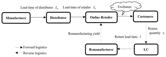
Figure 1.
The online closed-loop supply chain system.
3.1. Demand and Return Model
In an online CLSC with return and replacement in e-commerce, the market demand process for a particular product, , adheres to a first-order autoregressive AR (1) model:
where denotes the constant term. represents the auto-regression coefficient. is an independently and identically distributed normal random variable with mean zero and variance, . Lee et al. [42,43] demonstrated that the majority of products exhibit positive auto-regression correlation coefficients in demand. Consequently, the auto-regression coefficient is established as . The expectation and variance of demand are calculated: and .
In e-business, the effective management of consumer returns and replacements as critical operations for online retailers, is essential to maintaining customer satisfaction and loyalty. Consumers are empowered to initiate replacements for purchases that have quality problems or do not meet their expectations, often incurring only a minuscule proportion of the original cost. To streamline the online CLSC models, we make an assumption that the online retailer only and exclusively provides a replacement service for consumers to control the operational costs. Thereafter, the logistics center is tasked with gathering returned items from consumers and conveying them to the remanufacturer. Upon receipt of the returns by the remanufacturing department, the online retailer promptly acknowledges the transaction by confirming the return and replacement information. There is no information asymmetry between the online retailer and the remanufacturer. The online retailer needs to immediately facilitate the reshipment of new products after confirming the replacement requirement from consumers, thereby directly increasing the total demand faced by the online retailer. We make the assumption that all products subject to reshipment are in intact condition. Accordingly, the replacement volume is determined primarily by the genuine market demand quantity and the replacement rate.
The online retailer satisfies consumer orders by dispatching the true demand amount at the end of period . The e-tailer discerns the volume of product replacements at the start of period , where denotes the replacement rate. is the random disturbance term of the replacement quantity. Assume that shock term, , has no relation with the online market demand, . Then, the covariances are zero: . Moreover, a minor probability of a negative replacement quantity stems from a substantial constant term in demand.
When the remanufacturer receives returns at period , the yield from remanufacturing is anticipated to be , where represents the average yield rate achieved by the remanufacturer. is the stochastic disturbance term associated with the remanufacturing quantity. For the model simplicity, we exclude the random shock from the subsequent derivations. The overall volume dispatched by the remanufacturer to the e-tailer, , along with the manufacturing details, is fully known to the e-tailer. This study applies the simplifying assumption that the remanufacturing’s time delay is negligible, thereby streamlining the supply chain model. Assume that the replenishment of remanufactured products occurs instantaneously. A similar assumption can be found in Gao et al. [8]. Upon the completion of the remanufacturing process, the remanufacturer promptly notifies the retailer. Consequently, there is no information asymmetry between the e-tailer and remanufacturer. Remanufactured products are subsequently integrated into the e-tailer’s inventory to partially meet market demand, under the assumption that these remanufactured items perform equivalently to new products [8,44]. Thus, the total demand for the e-tailer during period can be articulated as:
where is the total demand, is the market demand, is the return and replacement quantity, and is the remanufacturing quantity.
3.2. Ordering Process
The order-up-to inventory strategy is a well-established strategy aimed at minimizing the total discounted costs associated with shortages and holdings. Given its cost-effectiveness, the order-up-to policy is broadly acknowledged as a locally optimal strategy. This paper assumes that both the e-tailer and the distributor utilize the order-up-to policy to determine the ordering. The ordering quantities for the e-tailer and the distributor are and , respectively, as follows:
The order-up-to level, , at each period can be calculated as , where is the safety stock kept to meet the anticipated lead time demand, derived as , and . is the predicted variance of forecasting error in periods with . denotes the safety factor with for normally distributed random variable . and refer to the unit holding and shortage costs, respectively.
Lemma 1.
The standard deviations of the estimating errors for the total lead time demand of the distributor and online retailer in online CLSC remain invariable as time progresses.
Proof.
See Appendix A. □
By substituting into (3) and,(4) we derive the ordering levels for both the e-tailer and the distributor as follows:
4. Ordering Decisions
In the section, we delineate the ordering decisions for both e-tailer and distributor. The online retailer and the distributor both leverage the same predicting method to project the average lead time demand.
4.1. Online Retailer’s Ordering Decision
The estimation of the AR (1) demand process, , in the minimum mean squared error (MMSE) forecasting technique, is given by . denotes the prediction of the overall demand for the e-tailer. From (2), the estimation of demand is derived in the formulation as . The market demand in period can be recursively formulated as , where is set as .
To determine the ordering quantity, the online retailer must first predict the overall lead time demand. The e-tailer utilizes the optimal MMSE estimation technique for forecasting, when the ordering lead time exceeds the return lead time. The total demand encompasses unknown information necessitating estimation in the ordering decisions for the retailer. Nevertheless, when the e-tailer’s lead time is less than the return lead time, the total lead time demand encompasses demand information known to the retailer. Accordingly, the interplay between the two lead times can significantly affect the order management and the operational performance.
The e-tailer forecasts the market lead time demand based on the demand information of period . The demand at period has already been actualized before , when . However, the demand of period is unknown to the e-tailer, necessitating prediction when . Then, the forecasting total market demand at period is:
Thus, the prediction of total lead time demand for the e-tailer is:
Lemma 1 proves that . Thus, by substituting (8) into(5), the order quantity of the online retailer in period is formulated as follows:
where .
4.2. Distributor’s Ordering Decision
IS can significantly influence a distributor’s order decisions by affecting their ability to forecast demand, manage inventory, and optimize profitability. In this section, we investigate the distributor’s ordering strategies in different IS scenarios.
When the online retailer chooses not to share any information with the upstream enterprises, the distributor obtains only the ordering information, , delivered by the e-tailer. Then, the return variation, , and the demand variation, , are observed by the e-tailer but unavailable to the distributor. The distributor derives the estimated lead time demand, , based on without the demand and return data. is the demand prediction of the distributor without IS formulated as . The predicted average lead time demand over periods is:
According to Lemma 1, the ordering volume, , of the distributor in period is:
By integrating Equation (10) into (11), we derive the order quantity for the distributor in the absence of IS:
When the online retailer decides to disclose only demand-related data to the upstream partners, the distributor measures the estimating lead time demand, , according to the e-tailer’s order and demand variation information. When only demand information is shared, is the demand of the distributor, as follows:
In the setting where only return information is shared, the distributor measures the estimating lead time demand, , grounded on the e-tailer’s order and return variation data. is the distributor’s demand with return and replacement IS:
Under a full IS framework, upstream enterprises have access to both demand and return information. The distributor quantifies the estimating lead time demand grounded on the order , market demand variation , and return variation . represents the distributor’s demand when sharing full information:
5. Quantification of Bullwhip Effect and Inventory Cost
This section delineates the quantification of bullwhip effect and inventory cost across distinctive IS mechanisms under two supply chain contexts: and .
5.1. Bullwhip Effect
The IS mechanisms do not affect the bullwhip effects or ordering policies of the online retailer [1,37,43]. The bullwhip effect for the retailer can be formulated as the ratio of the variances of order quantity and market demand .
If the e-tailer adopts the MMSE forecasting technique and the order-up-to inventory policy, the expression of the order variances can be formulated as . When , the order variance for the e-tailer is:
When , the order variance for the e-tailer is:
The distinct IS mechanisms exert a significant influence solely on the ordering decisions and bullwhip effects of the distributor. The bullwhip effects under diverse IS settings are predominantly dictated by the distributor’s order variances, . The order variances of the distributor in four IS mechanisms are derived from (12), (13), (14), and (15). The equations of can be seen in Appendix B.
5.2. Expected Cost
This section investigates the expected inventory costs for the distributor across the distinctive IS scenarios.
In an online CLSC involving return and replacement, the inventory cost for the distributor with full IS can be formulated as:
where denotes the optimal order-up-to level for the distributor, . represents the actual distribution of . The right loss function, , follows a standard normal distribution, denoted as , which has the following property: .
Without IS, the expected cost of the distributor, , is , where and . Obviously, it can be deduced from and that . Consequently, the implementation of a full IS strategy, which encompasses both demand and return and replacement information, is anticipated to exert a significant reduction in the inventory costs of the distributor.
With demand IS, the expected cost of the distributor, , is , where and . From and , we have . Therefore, the inventory cost associated with only demand IS is greater than that when both demand and return and replacement information are shared. This comparative analysis underscores the importance of incorporating return and replacement information into the distributor’s decision-making process.
With return and replacement IS, the expected cost of the distributor, , is , where and . Clearly, when the online retailer shares only return and replacement information, the distributor is unable to attain the lowest possible inventory cost. This scenario highlights the insufficiency of return and replacement information alone in optimizing inventory management. Consequently, the sharing of demand information emerges as an effective strategy for the distributor to reduce inventory costs.
6. Impacts of Information Sharing and Return Rate
In this section, we conduct analyses of the optimal IS decisions that could be made in various supply chain scenarios. Specifically, we examine the influence of the replacement rate on operational efficiencies.
6.1. Value of Information Sharing on Bullwhip Effects
A comparative analysis of the ordering variances in four distinct IS settings under two supply chain contexts is conducted, revealing the differential impact of each IS strategy on the distributor’s bullwhip effects and inventory management. To provide a reference point, the order variance in the absence of IS serves as the benchmark. By comparing the order variances against the benchmark, we can more effectively evaluate the different efficacy of each IS mechanism on bullwhip reduction. The order variance differences in different information setting are set as , , and . The results are interpreted as the effect of demand and/or return information on bullwhip effects as compared to that without IS.
When , we derive variance differences that , , and . Therefore, either sharing demand information or return information can restrain bullwhip effects.
Proposition 1.
When e-tailer’s lead time exceeds the return lead time, sharing either demand or return information can attenuate the distributor’s bullwhip effect in online CLSC.
Proof.
see Appendix B. □
Proposition 1 suggests that sharing demand or return information mitigates the bullwhip effect when . Specifically, when both categories of information are disclosed concurrently, the distributor will experience the most significant reduction in the bullwhip effect. In pursuit of mitigating the bullwhip effect and curbing information distortion, the most advantageous strategy for IS in the online CLSC is comprehensive IS. As a result, bolstering collaborative efforts among the various stakeholders in online CLSC is imperative. The influence of parameters on the differences of ordering variances when is depicted in Figure 2 and Figure 3.
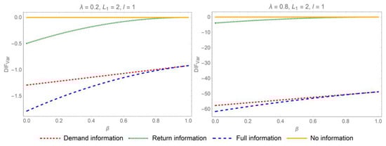
Figure 2.
Impact of the auto-regression coefficient on bullwhip reduction when the e-tailer’s lead time exceeds the return lead time.
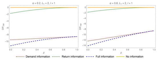
Figure 3.
Impact of the replacement rate on bullwhip effect reduction when the e-tailer’s lead time exceeds the return lead time.
When , we derive variance differences: . However, and depend on , , , , , and . Consequently, the dissemination of return and replacement information can serve to curb the bullwhip effects. The impact of demand information on bullwhip effects depends on the auto-regression coefficient, the replacement rate, the remanufacturing yield rate, the lead times, and the random shocks.
Proposition 2.
In scenarios where the e-tailer’s lead time is less than the return lead time, the sharing of return and replacement information can effectively diminish the bullwhip effect encountered by the distributor in the online CLSC.
Proof.
see Appendix B. □
Proposition 2 suggests that, when , the product return and replacement information plays a pivotal role in mitigating the bullwhip effect, whereas the impact of demand IS on bullwhip effects cannot be directly observed from the formulas. Accordingly, the demand IS mechanism is graphically represented in Figure 4 and Figure 5.
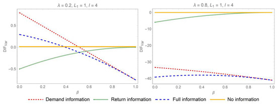
Figure 4.
Impact of the auto-regression coefficient on bullwhip effect reduction when the return lead time exceeds the e-tailer’s lead time.
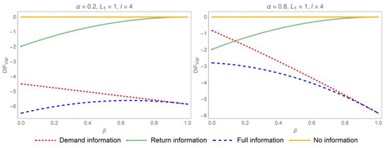
Figure 5.
Impact of replacement rate on bullwhip effect reduction when the return lead time exceeds the e-tailer’s lead time.
In order to quantify the extent of bullwhip effect mitigation when and , we conduct an analytical examination of the relationship between the reduction in the bullwhip effect attributable to IS and several key influencing parameters. To simplify the illustration, we set . Figure 2, Figure 3, Figure 4 and Figure 5 graphically depict the impacts of the yield rate, the replacement rate, and the auto-regression coefficient on the extent to which the bullwhip effect is mitigated from IS. The Y-axis, , illustrates the bullwhip effect reduction from demand and/or return IS in two supply chain contexts. All in all, when the online retailer’s lead time is greater than the return lead time, the strategic implementation of the demand and return IS can significantly mitigate the bullwhip effect. On this occasion, full IS is theorized to result in the lowest bullwhip effect compared to other IS strategies. Contrastively, when the e-tailer’s lead time is less than the return lead time, return and replacement IS still exerts a positive influence on bullwhip reduction. However, demand information has a counterintuitive and distinctive effect on bullwhip effects, especially when demand is lowly auto-correlated.
Figure 2 and Figure 4 reveal that the reduction magnitude is positively influenced by the auto-regression coefficient regardless of the interplay between the replenishment and return lead times. The reduction degree is positively affected by the auto-regression coefficient in two supply chain contexts. When demand exhibits high levels of auto-correlation, the potential for IS to mitigate the bullwhip effect is significantly enhanced. Figure 3 and Figure 5 depict the effect of the replacement rate on the mitigation extent of bullwhip effect from demand IS in two supply chain contexts. When the online retailer’s lead time is larger than the return lead time, the efficacy of demand IS in suppressing information distortion is more pronounced with a high replacement rate. Contrastively, when the online retailer’s lead time is less than the return lead time, a lower replacement rate has a more prominent effectiveness of demand IS in mitigating the bullwhip.
Figure 2, Figure 3, Figure 4 and Figure 5 disclose the different influences of the yield rate on the mitigation extent of bullwhip effect from demand and/or return IS in two supply chain contexts. When the online retailer’s lead time is larger than the return lead time, the reduction extent of the bullwhip effect from demand and return information decreases as the yield rate increases. Contrastively, when the e-tailer’s lead time is shorter than the return period, the yield rate will be positively related to the reduction extent of the bullwhip effect from demand information and negatively related with that from the return and replacement information.
Figure 4 indicates that the demand IS may deteriorate the operational performance. Extensive research has been conducted to mitigate distortions in market dynamics across supply chain networks through IS. The positive impact of sharing demand information on reducing the bullwhip effect has been well documented through numerous empirical and theoretical studies. However, we present a counterintuitive finding: when an online retailer shares only demand information, omitting product return and replacement details, the supply chain may experience an intensified bullwhip effect compared to scenarios without any IS. Moreover, this counterintuitive conclusion is rational. Product replacement inherently prompts decision-makers to place larger orders to offset anticipated inventory losses. This sign of amplifying demand is conveyed to upstream enterprises via e-tailer’s ordering, thereby amplifying information volatility in the online CLSC. Specifically, if the e-tailer does not share product return and replacement information with other supply chain partners, then the distributor is unable to fully understand the components that make up the total demand. Consequently, the demand forecasts developed by the distributor are prone to deviate from the actual demand distribution. By examining Equation (9), the variability in the estimated replacement quantity appears to be greater when compared to when . In other words, the information variability resulting from the product return and replacement is more drastic when the return lead time exceeds the e-tailer’s lead time. Accordingly, when there is a significant information mutation due to returns and replacements, sharing demand information alone may not be sufficient to restrain the bullwhip effects.
It is noteworthy that the influence of demand IS on the operational performance fluctuates considerably depending on the interplay between the replenishment lead time and the return lead time. When the return lead time is less than the replenishment lead time, the dampening impact on the bullwhip effect is more pronounced. Nevertheless, when return lead time exceeds the replenishment lead time, the bullwhip effect may be amplified. This could be due to the retailer’s capacity to swiftly modify demand forecasts and ordering choices when returns and replacements happen in a single ordering cycle. Additionally, having access to anticipated demand data can help mitigate the signal of rising demand and, as a result, bolster the information stability of online CLSCs.
6.2. Value of Information Sharing on Inventory Cost
We conducted a comparative analysis of the inventory costs under four distinct IS mechanisms in two supply chain contexts, manifesting the differential impact of each IS strategy on the distributor’s expected inventory costs. As a reference point, the inventory cost with full IS is designated as the benchmark. By comparing the inventory costs against the benchmark, we can more effectively evaluate the different efficacy of each IS mechanism on cost reduction.
The inventory cost differences in four information setting are set as , , and . The findings illustrate the impacts of alternative IS mechanisms on anticipated inventory costs relative to complete IS. In two supply chain contexts, we compute cost differences that , , and . Therefore, either sharing demand information or return information can reduce the expected cost in online CLSCs, regardless of the interplay between an e-tailer’s replenishment and return lead times.
Proposition 3.
The implementation of either demand IS or return IS is projected to result in a reduction in the expected inventory costs of the distributor in two supply chain contexts.
Proof.
see Appendix A. □
Proposition 3 demonstrates that complete IS is the optimal mechanism for the distributor to minimize the inventory cost in two supply chain settings. The beneficial impact of IS on reducing expected costs has been extensively validated by a multitude of studies. While IS may not confer direct benefits to the online retailer, it consistently proves advantageous for the upstream provider, such as the distributor.
To quantitatively assess the extent of the cost savings achievable through IS, we graphically illustrate the relationships between the cost reduction and the auto-regression coefficient, the replacement rate, and the yield rate, as shown in Figure 6, Figure 7, Figure 8 and Figure 9. The Y-axis, , represents cost reduction in different IS mechanisms. First of all, demand or return IS serves as an efficacious strategy for reducing inventory costs in two supply chain contexts. By facilitating the transparency of demand and return information, supply chain participants can make more precise inventory management decisions, leading to a decrease in inventory costs. Similarly, the extent of cost reduction is positively correlated with the auto-regression coefficient. The impact of IS on reducing costs is more pronounced when demand exhibits a high degree of auto-correlation. Moreover, as the replacement rate increases, the potential for cost reduction through the sharing of demand information also rises. However, returns and replacements often signify the unnecessary consumption of resources, leading to inefficiencies and disruptions in ordering decisions. Therefore, it is strategically advisable to minimize replacement rates whenever feasible. When e-tailer’s lead time surpasses the return lead time, a lower yield rate, which indicates a less efficient reintegration of returned products into the supply chain, paradoxically leads to greater potential savings in inventory costs through IS. This counterintuitive outcome suggests that, under conditions of lower yield rates, there is a heightened incentive to improve inventory management practices to offset the inefficiencies associated with product returns. However, this interplay may not persist if demand exhibits high auto-correlation, as the strong predictability of future demand from historical patterns could diminish the relative impact of IS on cost savings.
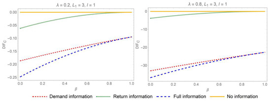
Figure 6.
Impact of the auto-regression coefficient on cost reduction when the e-tailer’s lead time exceeds the return lead time.
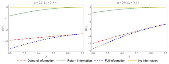
Figure 7.
Impact of the replacement rate on cost reduction when the e-tailer’s lead time exceeds the return lead time.
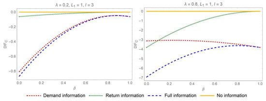
Figure 8.
Impact of the auto-regression coefficient on cost reduction when the return lead time exceeds the e-tailer’s lead time.
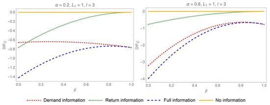
Figure 9.
Impact of the replacement rate on cost reduction when the return lead time exceeds the e-tailer’s lead time.
6.3. Impact of Replacement Rate
We examine how the replacement rate and the yield rate impact the bullwhip effect and inventory cost for the e-tailer. Recognizing the unique characteristics of online CLSCs is essential for developing effective strategies and operational tactics that enhance performance.
Proposition 4.
The effect of yield rate substantiates that, when and , in the interval, , , and . Hence, and are negatively related with the replacement rate, .
Proposition 4 shows that a higher yield rate in remanufacturing will lower the bullwhip effect and expected cost of the e-tailer in an online CLSC. The counterintuitive viewpoint is actually rational. Remanufactured products, when subjected to rigorous quality control and restoration processes, are capable of fulfilling market demand to an extent comparable to that of newly produced goods. An increased yield in the remanufacturing process signifies that a higher volume of returned items will be reintegrated into the e-tailer’s stock. This reintegration serves to partially offset the fluctuations in market demand, thereby mitigating the information distortion. Furthermore, online retailers have the capability to revise the projections of future true demand with greater timeliness, thereby enhancing the accuracy of the ordering decisions. Previous studies have demonstrated the restraining effect of reverse logistics on the bullwhip effects.
Proposition 5.
The influence of replacement rate on e-tailer’s ordering variance exhibits that, when and , in the interval, and . Hence, is positively related with the replacement rate, .
Proposition 6.
The influence of replacement rate on e-tailer’s inventory cost exhibits several distinct properties:
- (a)
- When , in the interval, and . Hence, is positively related with the replacement rate, .
- (b)
- When , in the interval, , is not related to the replacement rate, .
Propositions 5 and 6 posit that returns and replacements in e-retail inherently contribute to an increase in information volatility and inventory costs for the retailer, thereby potentially impairing the operational efficiencies. In the context of online CLSCs, product replacement tends to inflate the actual demand experienced by the e-tailer and subsequently transmits a sign of heightened demand to upstream suppliers. Therefore, the defective products will suffer more severe bullwhip effects and higher inventory costs compared to intact ones in e-commerce.
7. Conclusions
7.1. Theoretical Contribution
This research explores the optimal IS mechanisms in online CLSC systems. This study offers a comprehensive examination of the impact of product returns and replacements on the bullwhip effect and inventory costs, providing fresh insights into the operational dynamics of online CLSCs. We uncover strategies that can enhance both economic efficiency and customer satisfaction, thereby contributing to the overall effectiveness of supply chain management. The key contributions of this research are multifaceted and are summarized here.
First, the results underscore the vital importance of incorporating return and replacement information into supply chain management practices. It is essential for distributors and online retailers to identify the most effective IS decisions based on particular supply chain contexts when forming robust supply chain partnerships. A distributor who fails to account for the return and replacement dynamics in e-business may experience detrimental operational performance. The transparency of return and replacement information is crucial for enhancing the operational efficiency of online CLSCs. By leveraging this information, distributors and retailers can make more informed decisions regarding demand forecasting and inventory management. This can lead to reduced operational costs and a lower bullwhip effect.
Second, online CLSCs exhibit distinctive anomalies when the return lead time extends beyond an e-tailer’s lead time. Specifically, sharing demand information can unexpectedly exacerbate the bullwhip effect, which runs counter to the prevailing view from prior theoretical research that IS generally boosts supply chain performance [40,42,43]. This counterintuitive outcome suggests that the dynamics of online CLSCs may be more complex than initially understood, and that the benefits of IS are not universally applicable across all scenarios.
Third, under the condition where the e-tailer’s lead time exceeds the return lead time, sharing both return and demand information can be a significant advantage for the distributor, minimizing the bullwhip effect and the inventory cost. This comprehensive IS allows for a more accurate assessment of market dynamics and consumer behavior, leading to improved inventory management and a more responsive supply chain [1,36,37,54]. This finding underscores the importance of a holistic approach to information management in supply chains, where detailed and timely data can lead to better decision making and improved performance. The critical role of comprehensive IS in bolstering supply chain efficiency is well established in both theoretical [28] and empirical research [46,47,48].
Fourth, the analysis contributes significant knowledge for managers on enhancing the reduction effects of bullwhip and inventory costs from IS in an online CLSC. The efficacy of information transparency in mitigating the bullwhip effect and reducing inventory costs is significantly modulated by the auto-regression coefficient [43], the replacement rate, and the lead times. These findings highlight the complex interplay between supply chain contexts and the efficacy of IS in supply chain management.
Finally, this study investigates the impact of exchange behaviors in e-commerce on CLSCs. However, it is evident that returns and exchanges in reverse logistics have significantly different effects on operational performance. The findings of this research indicate that product exchanges amplify the bullwhip effect and increase inventory costs, which contrasts with the conclusions drawn from studies on product returns, which suggest that returns can mitigate the bullwhip effect in supply chains [9,28].
7.2. Managerial Implication
This research provides valuable practical guidance for managers aiming to optimize their IS practices and enhance supply chain resilience in the dynamic of online CLSCs. By offering actionable insights for supply chain management and information decision making, this study equips managers with the strategies necessary to navigate the challenges of modern supply chain operations. The key managerial implications of this research are summarized here.
First, the study highlights the critical need for supply chain managers to integrate detailed return and replacement data into their decision-making processes. By sharing detailed product return information, both manufacturers and online retailers can achieve better demand forecasting, improved inventory management, and enhanced overall operational efficiency. Upstream companies should develop collaborative partnerships with other supply chain partners and invest in advanced information systems capable of capturing and analyzing detailed return and replacement data. These systems provide real-time insights that facilitate quick decision making and improve supply chain responsiveness.
Second, supply chain managers need to optimize their IS decisions according to different supply chain contexts. If a supply chain’s objective is to directly maximize cost reduction, the optimal mechanism is full IS. This strategy ensures that all relevant data are leveraged to make informed decisions, thereby enhancing supply chain efficiency and potentially increasing profitability. Moreover, the study also reveals a critical insight for supply chain managers operating in environments where the primary goal of an online CLSC is to minimize information distortion; here, the potential optimal strategy is to share only return information and not demand information when return lead times exceed e-tailer’s lead times. This counterintuitive finding suggests that, in certain contexts, selective IS can be more effective than comprehensive sharing in achieving supply chain objectives.
Finally, it is imperative for online retailers to strategically control the replacement rate, which can be achieved by partnering with higher-quality suppliers. Online retailers should implement rigorous quality assurance programs to further enhance the reliability of products. For instance, regular quality checks, audits, and performance evaluations of suppliers can ensure consistent product quality and reduce the likelihood of defects. By sourcing products from suppliers with a proven track record of quality and reliability, online retailers can potentially reduce the incidence of defective products, thereby lowering the replacement rate. This reduction in product exchange is expected to attenuate the bullwhip effect, leading to a decrease in inventory costs and an increase in supply chain efficiency.
7.3. Limitations
The assumptions utilized in this study streamline the analysis of supply chain dynamics, yet they also impose certain limitations. First, the assumption that remanufactured items perform equivalently to new products may not fully capture the potential variability in product quality and reliability. In practice, remanufactured items might exhibit slightly lower performance or durability, which could influence customer satisfaction and inventory management decisions. Second, the study assumes that remanufacturing time delays are negligible, disregarding the complexities and potential delays intrinsic to the remanufacturing process. These overlooked delays can compromise the precision of demand forecasts and inventory levels, possibly resulting in stockouts or overstock situations. Third, the assumption posits no information asymmetry between the e-tailer and the remanufacturer, which may not mirror the actual supply chain operations where information disparities are prevalent due to varying data access, communication lags, or strategic behaviors. This discrepancy can lead to suboptimal coordination and synchronization within the supply chain. Fourth, the immediate reshipment of new products after confirming replacement requirements may not always be feasible due to logistical constraints, processing times, or supply availability. This could lead to unrealistic expectations for customer service levels and operational efficiency. Fifth, the study also simplifies the model by assuming that both the e-tailer and the distributor utilize the MMSE forecasting method. In bullwhip effect research, minimum mean squared error (MMSE), moving average (MA), and exponential smoothing (ES) are the most common forecasting methods. Each forecasting method has distinct advantages and limitations in demand forecasting. MMSE achieves the lowest prediction error and highest accuracy but has a complex model structure, complicating the analysis of the bullwhip effect and inventory cost properties. Sixth, we assume that a minor probability of a negative replacement quantity stems from a substantial constant term in demand. However, in practice, incorrect shipping orders and quantities are indeed a common phenomenon in e-commerce. When a negative replacement quantity occurs, it implies that, in addition to the quantity required by the order, the retailer has shipped extra products to the consumer. This typically indicates an error in the retailer’s order fulfillment, which is an issue that must be avoided. Finally, the assumption that redelivered items are in perfect condition and consumers will not initiate a second-round return process overlooks the possibility of multiple returns due to dissatisfaction or product issues. This could result in underestimating the complexity of managing returns and exchanges, potentially leading to higher costs and reduced customer satisfaction.
Future research could address these limitations by incorporating more nuanced models that account for the potential variability in remanufactured product quality and the inherent delays in the remanufacturing process. Investigating the impact of information asymmetry and developing robust IS mechanisms could enhance supply chain coordination and synchronization. Additionally, exploring different inventory management and forecasting strategies could provide more realistic insights into supply chain dynamics. Future studies could also consider the potential for multiple rounds of returns and exchanges, developing more comprehensive models to manage these complexities effectively. By addressing these limitations, future research can contribute to a more robust and realistic understanding of supply chain operations, ultimately leading to improved decision making and operational efficiency.
Author Contributions
All authors contributed to all aspects of the study, reviewed the results. All authors have read and agreed to the published version of the manuscript.
Funding
This work was supported by the Youth Program of National Natural Science Foundation of China (72202216), and the Major Program of National Natural Science Foundation of China (72192830/72192833/72192834).
Data Availability Statement
The original contributions presented in the study are included in the article.
Conflicts of Interest
The authors declare no conflicts of interest.
Abbreviations
The following abbreviations are used in this manuscript:
| IS | information sharing |
| CLSC | closed-loop supply chain |
| MMSE | minimum mean squared error |
| MA | moving average |
| ES | exponential smoothing |
| AR | auto-regressive |
| Y | yes |
| N | no |
Appendix A
The variances of forecasting errors for the e-tailer are derived as follows.
When ,
When ,
The variances of the forecasting errors of the distributor, , , and are derived as follows.
When ,
When ,
where
When ,
where .
When ,
where
When ,
where .
When ,
where .
Appendix B
The order variances for the distributor , , and are derived as follows.
When ,
When ,
When ,
where when . It is formulated as:
When ,
where when . It is formulated as:
When ,
where when . It is formulated as:
When ,
where when . It is formulated as:
This completes the proof.
References
- Gao, D.; Wang, N.; Jiang, B.; Gao, J.; Yang, Z. Value of information sharing in online retail supply chain considering product loss. IEEE Trans. Eng. Manag. 2022, 69, 2155–2172. [Google Scholar] [CrossRef]
- Niu, Y.; Wu, J.; Jiang, S.; Jiang, Z. The bullwhip effect in servitized manufacturers. Manag. Sci. 2024, 71, 1–20. [Google Scholar] [CrossRef]
- Cui, G.; Imura, N.; Nishinari, K. Should firms invest in demand forecasting? Benefits of improving forecasting accuracy on order smoothing, dual-sourcing and multi-stage supply chain problems. Int. J. Prod. Res. 2025. [Google Scholar] [CrossRef]
- Lingkon, M. Bullwhip effect on closed-loop supply chain considering lead time and return rate: A study from the perspective of Bangladesh. Decis. Sci. Lett. 2024, 13, 565–586. [Google Scholar] [CrossRef]
- Yin, X.; Tang, W. The value of market information and the bullwhip effect. J. Oper. Res. Soc. 2024, 75, 2241–2252. [Google Scholar] [CrossRef]
- Tombido, L.; Louw, L.; van Eeden, J. The bullwhip effect in closed-loop supply chains: A comparison of series and divergent networks. J. Remanuf. 2020, 10, 207–238. [Google Scholar] [CrossRef]
- Chen, F.; Simchi-Levi, D. Quantifying the Bullwhip Effect in a Simple Supply Chain: The Impact of Forecasting, Lead Times, and Information. Manag. Sci. 2000, 46, 436–443. [Google Scholar] [CrossRef]
- Gao, D.; Wang, N.; He, Z.; Zhou, L. Analysis of bullwhip effect and inventory cost in the online closed-loop supply chain. Int. J. Prod. Res. 2023, 61, 6808–6828. [Google Scholar] [CrossRef]
- Hosoda, T.; Disney, S.M. A unified theory of the dynamics of closed-loop supply chains. Eur. J. Oper. Res. 2018, 269, 313–326. [Google Scholar] [CrossRef]
- Papanagnou, C.I. Measuring and eliminating the bullwhip in closed loop supply chains using control theory and Internet of Things. Ann. Oper. Res. 2022, 310, 153–170. [Google Scholar] [CrossRef]
- Udenio, M.; Vatamidou, E.; Fransoo, J.C. Exponential smoothing forecasts: Taming the bullwhip effect when demand is seasonal. Int. J. Prod. Res. 2023, 61, 1796–1813. [Google Scholar] [CrossRef]
- Darmawan, A.; Wong, H.W.; Fransoo, J. Supply chain network design with the presence of the bullwhip effect. Int. J. Prod. Econ. 2025, 286, 109668. [Google Scholar] [CrossRef]
- Li, Q.Y.; Gaalman, G.; Disney, S.M. Dynamic analysis of the proportional order-up-to policy with damped trend forecasts. Int. J. Prod. Econ. 2025, 285, 109612. [Google Scholar] [CrossRef]
- Patil, C.; Prabhu, V. Supply chain cash-flow bullwhip effect: An empirical investigation. Int. J. Prod. Econ. 2024, 267, 109065. [Google Scholar] [CrossRef]
- Singhal, V.; Wu, J. The Bullwhip Effect and Stock Returns. Prod. Oper. Manag. 2024, 33, 303–322. [Google Scholar] [CrossRef]
- Jalali, H.; Menezes, M.B. Product portfolio adjustments and the bullwhip effect: The impact of product introduction and retirement. Eur. J. Oper. Res. 2024, 318, 87–99. [Google Scholar] [CrossRef]
- Du, K.; Jia, F.; Chen, L. The impact of customers’ MD&A sentiment on the bullwhip effect: A dyadic buyer-supplier perspective. Int. J. Prod. Econ. 2025, 284, 109614. [Google Scholar]
- Giri, B.C.; Glock, C.H. The bullwhip effect in a manufacturing/remanufacturing supply chain under a price-induced non-standard ARMA(1,1) demand process. Eur. J. Oper. Res. 2022, 301, 458–472. [Google Scholar] [CrossRef]
- Tai, P.D.; Buddhakulsomsiri, J.; Duc, T.T.H. Revisiting measurement of compound bullwhip with asymmetric reference price. Comput. Ind. Eng. 2022, 172, 108510. [Google Scholar] [CrossRef]
- Dominguez, R.; Cannella, S.; Ponte, B.; Framinan, J.M. On the dynamics of closed-loop supply chains under remanufacturing lead time variability. Omega 2020, 97, 102106. [Google Scholar] [CrossRef]
- Tombido, L.; Louw, L.; van Eeden, J.; Zailani, S. A system dynamics model for the impact of capacity limits on the bullwhip effect (bwe) in a closed-loop system with remanufacturing. J. Remanuf. 2022, 12, 1–45. [Google Scholar] [CrossRef]
- Cannella, S.; Ponte, B.; Dominguez, R.; Framinan, J.M. Proportional order-up-to policies for closed-loop supply chains: The dynamic effects of inventory controllers. Int. J. Prod. Res. 2021, 59, 3323–3337. [Google Scholar] [CrossRef]
- Zhang, M.L.; Wang, Y.N.; Zhang, Y.J. Research on Supply Chain Coordination Decision Making under the Influence of Lead Time Based on System Dynamics. Systems 2024, 12, 32. [Google Scholar] [CrossRef]
- Ponte, B.; Framinan, J.M.; Cannella, S.; Dominguez, R. Quantifying the Bullwhip Effect in closed-loop supply chains: The interplay of information transparencies, return rates, and lead times. Int. J. Prod. Econ. 2020, 230, 107798. [Google Scholar] [CrossRef]
- Tombido, L.; Baihaqi, I. The impact of a substitution policy on the bullwhip effect in a closed loop supply chain with remanufacturing. J. Remanuf. 2020, 10, 177–205. [Google Scholar] [CrossRef]
- Ponte, B.; Cannella, S.; Dominguez, R.; Naim, M.M.; Syntetos, A.A. Quality grading of returns and the dynamics of remanufacturing. Int. J. Prod. Econ. 2021, 236, 108129. [Google Scholar] [CrossRef]
- Zhou, L.; Naim, M.M.; Disney, S.M. The impact of product returns and remanufacturing uncertainties on the dynamic performance of a multi-echelon closed-loop supply chain. Int. J. Prod. Econ. 2017, 183, 487–502. [Google Scholar] [CrossRef]
- Hosoda, T.; Disney, S.M.; Gavirneni, S. The impact of information sharing, random yield, correlation, and lead times in closed loop supply chains. Eur. J. Oper. Res. 2015, 246, 827–836. [Google Scholar] [CrossRef]
- Delavar, H.; Gilani, H.; Sahebi, H. A system dynamics approach to measure the effect of information sharing on manufacturing/remanufacturing systems’ performance. Int. J. Comput. Integr. Manuf. 2022, 35, 859–872. [Google Scholar] [CrossRef]
- Huang, F.; Pan, Y.; Zhao, Z.; Song, H.; Liu, Y.Y. Manufacturer Channel-Selection Strategy Considering Information Sharing Under Uncertain Demand. Systems 2025, 13, 108. [Google Scholar] [CrossRef]
- Jiao, L.L.; Deng, F.M. The Impact of Platform Information Sharing on Manufacturer's Choice of Online Distribution Mode and Green Investment. Systems 2024, 12, 127. [Google Scholar] [CrossRef]
- Nagaraja, C.H.; McElroy, T. The multivariate bullwhip effect. Eur. J. Oper. Res. 2018, 267, 96–106. [Google Scholar] [CrossRef]
- Teunter, R.H.; Babai, M.Z.; Bokhorst, J.A.; Syntetos, A.A. Revisiting the value of information sharing in two-stage supply chains. Eur. J. Oper. Res. 2018, 270, 1044–1052. [Google Scholar] [CrossRef]
- Sarkar, M.; Dey, B.K.; Ganguly, B.; Saxena, N.; Yadav, D.; Sarkar, B. The impact of information sharing and bullwhip effects on improving consumer services in dual-channel retailing. J. Retail. Consum. Serv. 2023, 73, 103307. [Google Scholar] [CrossRef]
- Hosoda, T.; Disney, S.M. On variance amplification in a three-echelon supply chain with minimum mean square error forecasting. Omega-Int. J. Manag. Sci. 2006, 34, 344–358. [Google Scholar] [CrossRef]
- Agrawal, S.; Sengupta, R.N.; Shanker, K. Impact of information sharing and lead time on bullwhip effect and on-hand inventory. Eur. J. Oper. Res. 2009, 192, 576–593. [Google Scholar] [CrossRef]
- Zhang, S.H.; Cheung, K.L. The impact of information sharing and advance order information on a supply chain with balanced ordering. Prod. Oper. Manag. 2015, 20, 253–267. [Google Scholar] [CrossRef]
- Ma, Y.; Wang, N.; Che, A.; Huang, Y.; Xu, J. The bullwhip effect under different information-sharing settings: A perspective on price-sensitive demand that incorporates price dynamics. Int. J. Prod. Res. 2013, 51, 3085–3116. [Google Scholar] [CrossRef]
- Wang, N.; Lu, J.; Feng, G.; Ma, Y.; Liang, H. The bullwhip effect on inventory under different information sharing settings based on price-sensitive demand. Int. J. Prod. Res. 2016, 54, 4043–4064. [Google Scholar] [CrossRef]
- Dai, H.; Li, J.; Yan, N.; Zhou, W. Bullwhip effect and supply chain costs with low- and high-quality information on inventory shrinkage. Eur. J. Oper. Res. 2016, 250, 457–469. [Google Scholar] [CrossRef]
- Yan, R.; Cao, Z. Product returns, asymmetric information, and firm performance. Int. J. Prod. Econ. 2017, 185, 211–222. [Google Scholar] [CrossRef]
- Lee, H.L.; Padmanabhan, V.; Whang, S. Information Distortion in a Supply Chain: The Bullwhip Effect. Manag. Sci. 1997, 43, 546–558. [Google Scholar] [CrossRef]
- Lee, H.L.; So, K.C.; Tang, C.S. The Value of Information Sharing in a Two-Level Supply Chain. Manag. Sci. 2000, 46, 626–643. [Google Scholar] [CrossRef]
- Atasu, A.; Toktay, L.B.; Van Wassenhove, L.N. How collection cost structure drives a manufacturer’s reverse channel choice. Prod. Oper. Manag. 2013, 22, 1089–1102. [Google Scholar] [CrossRef]
- Jena, S.K.; Sarmah, S. Price competition and co-operation in a duopoly closed-loop supply chain. Int. J. Prod. Econ. 2014, 156, 346–360. [Google Scholar] [CrossRef]
- Li, S.; Ragu-Nathan, B.; Ragu-Nathan, T.S.; Rao, S.S. The impact of supply chain management practices on competitive advantage and organizational performance. Omega 2006, 34, 107–124. [Google Scholar] [CrossRef]
- Zhou, H.; Womack, B.C. Supply chain practice and information sharing. J. Oper. Manag. 2007, 25, 1348–1365. [Google Scholar] [CrossRef]
- Prajogo, D.; Olhager, J. Supply chain integration and performance: The effects of long-term relationships, information technology and sharing, and logistics integration. Int. J. Prod. Econ. 2012, 135, 514–522. [Google Scholar] [CrossRef]
- Wang, X.; Disney, S.M. The bullwhip effect: Progress, trends and directions. Eur. J. Oper. Res. 2016, 250, 691–701. [Google Scholar] [CrossRef]
- Geary, S.; Disney, S.M.; Towill, D.R. On bullwhip in supply chains—Historical review, present practice and expected future impact. Int. J. Prod. Econ. 2006, 101, 2–18. [Google Scholar] [CrossRef]
- Sahin, F.; Robinson, E.P. Flow coordination and information sharing in supply chains: Review, implications, and directions for future research. Decis. Sci. 2002, 33, 505–536. [Google Scholar] [CrossRef]
- Yang, Y.; Lin, J.; Liu, G.; Zhou, L. The behavioural causes of bullwhip effect in supply chains: A systematic literature review. Int. J. Prod. Econ. 2021, 236, 108120. [Google Scholar] [CrossRef]
- Wang, C.X.; Webster, S. Channel coordination for a supply chain with a risk-neutral manufacturer and a loss-averse retailer. Decis. Sci. 2007, 38, 361–389. [Google Scholar] [CrossRef]
- Qamar, A.; Clegg, B.; Bryson, J.; Du, B. Risk mitigation, adaptability and sectoral resilience: Buffering in automotive supply chains prior & post disruption. Transp. Res. Part E 2025, 201, 104263. [Google Scholar]
Disclaimer/Publisher’s Note: The statements, opinions and data contained in all publications are solely those of the individual author(s) and contributor(s) and not of MDPI and/or the editor(s). MDPI and/or the editor(s) disclaim responsibility for any injury to people or property resulting from any ideas, methods, instructions or products referred to in the content. |
© 2025 by the authors. Licensee MDPI, Basel, Switzerland. This article is an open access article distributed under the terms and conditions of the Creative Commons Attribution (CC BY) license (https://creativecommons.org/licenses/by/4.0/).