Abstract
Mixed-flow assembly lines are widely employed in industrial manufacturing to handle diverse production tasks. For mixed flow assembly lines that involve mold changes and greater processing difficulties, there are currently two approaches: batch production and production according to order sequence. The first approach struggles to meet the processing constraints of workpieces with higher production difficulty, while the second approach requires the development of suitable scheduling schemes to balance mold changes and continuous processing. Therefore, under the second approach, developing an excellent scheduling scheme is a challenging problem. This study addresses the mixed-flow assembly shop scheduling problem, considering continuous processing and mold-changing constraints, by developing a multi-objective optimization model to minimize additional production time and customer waiting time. As this NP-hard problem poses significant challenges in solution space exploration, the conventional NSGA-II algorithm suffers from limited local search capability. To address this, we propose an enhanced NSGA-II algorithm (RLVNS-NSGA-II) integrating deep reinforcement learning. Our approach combines multiple neighborhood search operators with deep reinforcement learning, which dynamically utilizes population diversity and objective function data to guide and strengthen local search. Simulation experiments confirm that the proposed algorithm surpasses existing methods in local search performance. Compared to VNS-NSGA-II and SVNS-NSGA-II, the RLVNS-NSGA-II algorithm achieved hypervolume improvements ranging from 19.72% to 42.88% and 12.63% to 31.19%, respectively.
1. Introduction
Emerging digital technologies such as blockchain and AI-driven optimization transform supply-side production model from manufacturing resource allocation to personalized orders. To meet the challenges associated with personalized orders, manufacturing enterprises typically use mixed-flow assembly lines to complete production tasks in scenarios such as automotive assembly. Compared with traditional assembly lines, mixed-flow production lines can manufacture a variety of product types. Therefore, under the premise that high productivity, high efficiency, and high quality can increase competitiveness, the scheduling optimization problem of mixed-flow assembly lines has attracted widespread attention from both academia and industry [1,2,3]. The production approaches for mixed-flow assembly lines can generally be divided into two types. The first approach is to produce according to the order of the orders. The second approach involves categorizing similar products into the same batch for production. Both production approaches have their respective limitations. The first approach involves frequent changes in tools and molds, and existing research has pointed out the negative impacts of this approach [4]. Although the second approach reduces the frequency of tool and mold changes, different machined workpieces have varying levels of processing difficulty, making it challenging for some workstations to continuously process multiple workpieces that are more difficult to machine. To address these limitations, optimizing scheduling on mixed-flow assembly lines while considering both workstation overload and mold changes has become a critical issue for production-oriented enterprises.
The mixed-flow production line scheduling optimization problem is a subclass of flexible workshop scheduling optimization problems, and academia has conducted research on different mixed-flow assembly scenarios. Next, this article introduces the research status from the perspectives of the characteristics of the research scenarios and the characteristics of the solution methods. Wu et al. [5] developed a multi-stage model for personalized orders, whereas Shen et al. [6] and Zhang et al. [7] created balanced scheduling frameworks for shop floors. Su et al. [8] discussed the constraints of continuous processing in certain production scenarios and constructed a hybrid flow shop scheduling problem considering continuous processing and resource constraints. Wang et al. [9] further advanced the field by integrating logistics constraints with production scheduling. Many scholars have investigated production scheduling optimization for mixed-flow lines under multi-objective frameworks. For example, Guan et al. [10] constructed a multi-objective scheduling optimization model considering the continuous casting scenario, using iterative information to enhance the solving effectiveness of the heuristic algorithm. Laili et al. [11] examined flexible scheduling in shared manufacturing equipment scenarios and solved the resulting multi-objective problem. Zhang et al. [12] studied multi-objective scheduling for vehicle production under unexpected disruptions. Unlike most studies that focus on minimizing the makespan, Liu et al. [13] prioritized the optimization of assembly waiting time as the primary objective.
Currently, heuristic algorithms have emerged as a primary solution approach for mixed-flow assembly line scheduling problems with particular emphasis on enhancing local search mechanisms. For example, Geng et al. [14] developed an automated guided vehicle (AGV) compatible hybrid heuristic incorporating process skipping to optimize both global and local search performance. Wu et al. [15] addressed the long-cycle, high-energy-consumption characteristics of steel pipe production by developing a hybrid flow shop scheduling model considering batch processing and re-entrant flows, improving heuristic algorithms via a diversity-based local search mechanism. Wallrath et al. [16] studied a flow shop scheduling optimization problem that considers batch and resource allocation, using an improved heuristic algorithm for solving it. Gao et al. [17] implemented a digital twin-oriented local search operator for dynamic scheduling scenarios. Ding et al. [18] designed a multi-operator genetic algorithm specifically for resource-constrained flow shop scheduling. However, these studies focused primarily on refining local search rules without leveraging iterative algorithm data to guide heuristic optimization. Reinforcement learning (RL) offers potential through its self-learning capability via environmental interaction [19], showing promise for heuristic enhancement. Specifically, RL has been applied to parameter tuning, fitness evaluation, solution initialization, and local search operator selection [20]. Traditional random or exhaustive operator selection methods either risk missing optimal solutions or require excessive computation time [21]. To address this, several studies have adopted RL for operator selection, including: (1) Q-table-based hybrid heuristics by Yüksel et al. [22] and Li et al. [23] for local search decisions; and (2) Q-learning-guided PSO by Li et al. [24]. However, Q-table approaches suffer from adaptability constraints due to discrete state requirements. Deep reinforcement learning (DRL) resolves this limitation through deep learning. Ding et al. [25] developed a DRL-based parameter adaptation mechanism to balance global and local search, and Zheng et al. [26] used iterative algorithm states as DRL inputs to guide optimization. Yuan et al. [27] improved the genetic algorithm via deep reinforcement learning operators and designed a hybrid reward mechanism that combines delayed immediate rewards with global rewards. This paper summarizes the similarities and differences between existing studies and the present work, as outlined in Table 1. Among them, ✖ and ✔ indicate whether the literature did not consider/considered the elements, and ‘experience guidance’ means that the algorithm used effective information from the iterative process to guide subsequent algorithmic solutions.

Table 1.
Current and Previous Studies.
Prior research has rarely integrated workload balancing, efficiency, and delivery performance within scheduling models. From a methodological perspective, some studies have employed DRL-driven operators to leverage iterative optimization data for solving mixed-flow assembly line scheduling problems, but this idea has not yet been applied to solve the problem studied in this paper.
In mixed-flow assembly lines, consecutive processing of high-difficulty workpieces can cause overload constraints, reducing overall efficiency. To address this: (1) This study constructs a mixed-flow assembly line scheduling optimization model considering overload constraints, with objectives to minimize additional production time and delivery deviation (a multi-objective optimization problem). (2) To overcome NSGA-II’s computational complexity and weak local search, we enhance it with a DRL operator that utilizes real-time optimization data to direct search processes. The experimental results validate the algorithm’s superior performance.
2. Problem Description and Modeling
2.1. Problem Description
The growing diversification of market demand has driven widespread adoption of mixed-flow assembly lines in manufacturing enterprises. In contrast, this approach enhances production flexibility, but significant variations in workpiece processing complexity present operational challenges. Consecutive scheduling of high-complexity workpieces can induce overload constraints, resulting in unplanned production interruptions and degraded overall efficiency.
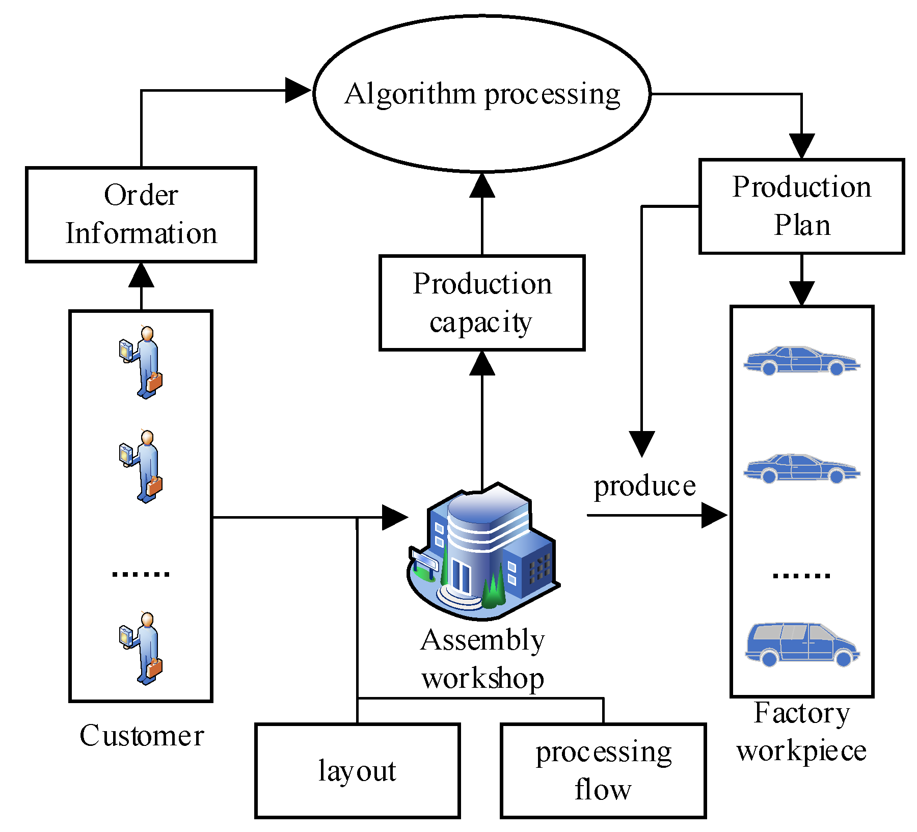
This study addresses a mixed-flow assembly line scheduling optimization problem, which is defined as follows: A manufacturing plant produces types of workpieces, where each type has configurations, denoted as . The layout and processing flow of the mixed-flow assembly line are known. These workpieces require types of components in total. The demand for each configuration is known and represented as . Customer orders are time sensitive, meaning that the quantity of each workpiece type to be delivered by period t is given by . Workstation tooling requirements and assembly times vary significantly across different workpiece configurations. Configurations with higher assembly complexity frequently induce overload constraint conditions. While assembly times remain fixed (being process-dependent), production efficiency improvements are achieved through sequence optimization, measured via two key metrics: (1) additional production time (combining overload and mold-changing durations) and (2) delivery deviation. The mixed-flow assembly line scheduling problem studied in this work is illustrated in Figure 1.

Figure 1.
Schematic diagram of the scheduling optimization problem for a mixed-flow assembly line.
To formulate the mixed-flow assembly line scheduling optimization problem, the following assumptions are made:
- The quantity of workpieces to be produced in each period is known in advance.
- Each assembly task at any workstation involves installing only one component.
- A workstation may handle one or multiple types of components.
- If a workstation consecutively assembles components exceeding a predefined difficulty threshold, overload time is needed, and production must wait until completion.
- If the component type changes at a workstation, a mold-changing time is incurred before the next assembly task can begin.
- Owing to uncertainties in order placement and delivery timelines, the customer waiting time in the model considers only scheduling-related delays (not external factors).
- No stochastic disruptions are considered; the completion time of each order depends solely on the production schedule.
2.2. Notations
This article constructs a mathematical model based on the optimization model of flexible workshop production scheduling. The key symbols and their definitions used in the mixed-flow assembly line scheduling problem with continuous processing constraints and mold-changing constraints are summarized in Table 2.
Table 2.
Symbol Definition Table.
2.3. Model formulation
The mixed-flow assembly line scheduling optimization model is a type of flexible workshop production scheduling optimization model, typically based on production scenarios such as electric vehicle manufacturing. Mixed-flow assembly line scheduling optimization traditionally prioritizes production efficiency and customer satisfaction. While improvements in the assembly process are beyond the scope of this study, we optimized the assembly sequence to reduce the additional production time. The integer programming model is formulated as follows:
Objective Functions:
Equation (1) calculates the additional production time , combining mold-changing time and overload processing time. The specific calculation approach is to sum the mold change waiting time and the overload processing time for each workpiece at each station for each cycle. Equation (2) computes the completion deviation , quantifying the discrepancy between the expected and actual production quantities per workpiece type per period. The specific calculation method calculates the difference between the order quantity for each configuration and the actual production quantity for each period.
The model incorporates virtual workpieces to represent workstation waiting states, occurring in two scenarios: (1) when awaiting upstream completion before starting, or (2) when awaiting downstream completion before finishing. These artificial elements enable computational efficiency while avoiding representation of actual workpieces.. They have zero processing time. When a virtual workpiece is processed at workstation , it indicates that the workstation is waiting for workpieces to arrive. For workstation , any workpiece processed in a position smaller than its workstation number is considered a virtual workpiece.
To accurately characterize the time constraints for workpieces entering workstations, we divide the constraints into two cases: one is when the workpiece is in the first position of a production cycle and at the first workstation, and the other is when the workpiece is in other positions of a production cycle or in the first position workpiece entering other workstations. For the first case, we have Constraints (3) and (4):
Constraint (3) indicates that the start time of the pipeline is 0 in any cycle. Constraint (4) represents the calculation constraint for the entry time of virtual workpieces.
For the second case, the entry time of a workpiece into a workstation is determined by the maximum completion time of the previous production positions across all workstations, as shown in Constraint (5):
Constraint (6) is established to characterize the mold-changing time between different production tasks. The specific calculation approach is to determine whether the task-related component is processed on , and whether this component is different from the component processed previously.
The processing start time for a workpiece at a workstation is determined by both its entry time and the required mold-changing time. Constraint (7) accordingly defines the workpiece processing start time:
The assembly time calculation accounts for both normal and overload conditions by distinguishing between two operational modes: (1) normal assembly time without overload, whose calculation constraint is the normal processing time. (2) Overload the assembly time when consecutive processing exceeds the threshold, which is calculated as the normal processing time plus the overload time. The assembly time calculation constraints are formulated as follows:
where represents the overload time penalty. The calculation of overload time depends on the number of consecutive workpieces processed at the workstation. When workstation j processes more than threshold of component , , and vice versa. Therefore, Constraint (10) is set as follows:
The completion time of workpiece at workstation depends on its start time and processing time. Therefore, constraint (11) is set to characterize the time when the workpiece leaves the workstation. The calculation method for the workpiece leaving the workstation is the start processing time plus the processing time.
Each accessory is completed by only one workstation. Therefore, constraint (12) is set to describe the processing constraints of the workstation and the operation:
In addition, any workstation can process one or more components. Constraint (13) is set as follows:
For the workpieces produced within each production cycle, constraint (14) is formulated to represent the output of workpieces during a given cycle. The calculation method for production during the period is the sum of the indicator variables. represents the indicator variable, returning 1 when is satisfied, and 0 otherwise.
Furthermore, the model has constraints on the values of decision variables (15):
3. Deep-Reinforcement Learning-Driven Enhanced NSGA-II
The nondominated sorting genetic algorithm (NSGA-II) represents an improved variant of genetic algorithms. Compared with conventional genetic algorithms, NSGA-II enhances its performance in solving multi-objective optimization problems through three key improvements: nondominated sorting, crowding distance comparison, and the elitist strategy. These characteristics render the approach particularly effective for solving the mixed-flow assembly line scheduling optimization problem under investigation. However, NSGA-II suffers from inherent limitations in local search capability, which manifests in two primary aspects when solving our proposed optimization model. First, the designed model requires decision-making for production planning of multiple workpiece types across various production cycles, resulting in an extensive solution space. Second, permutations of production sequences among nonoverloaded positions may not affect the objective function values, a characteristic further amplified in multi-objective optimization scenarios.
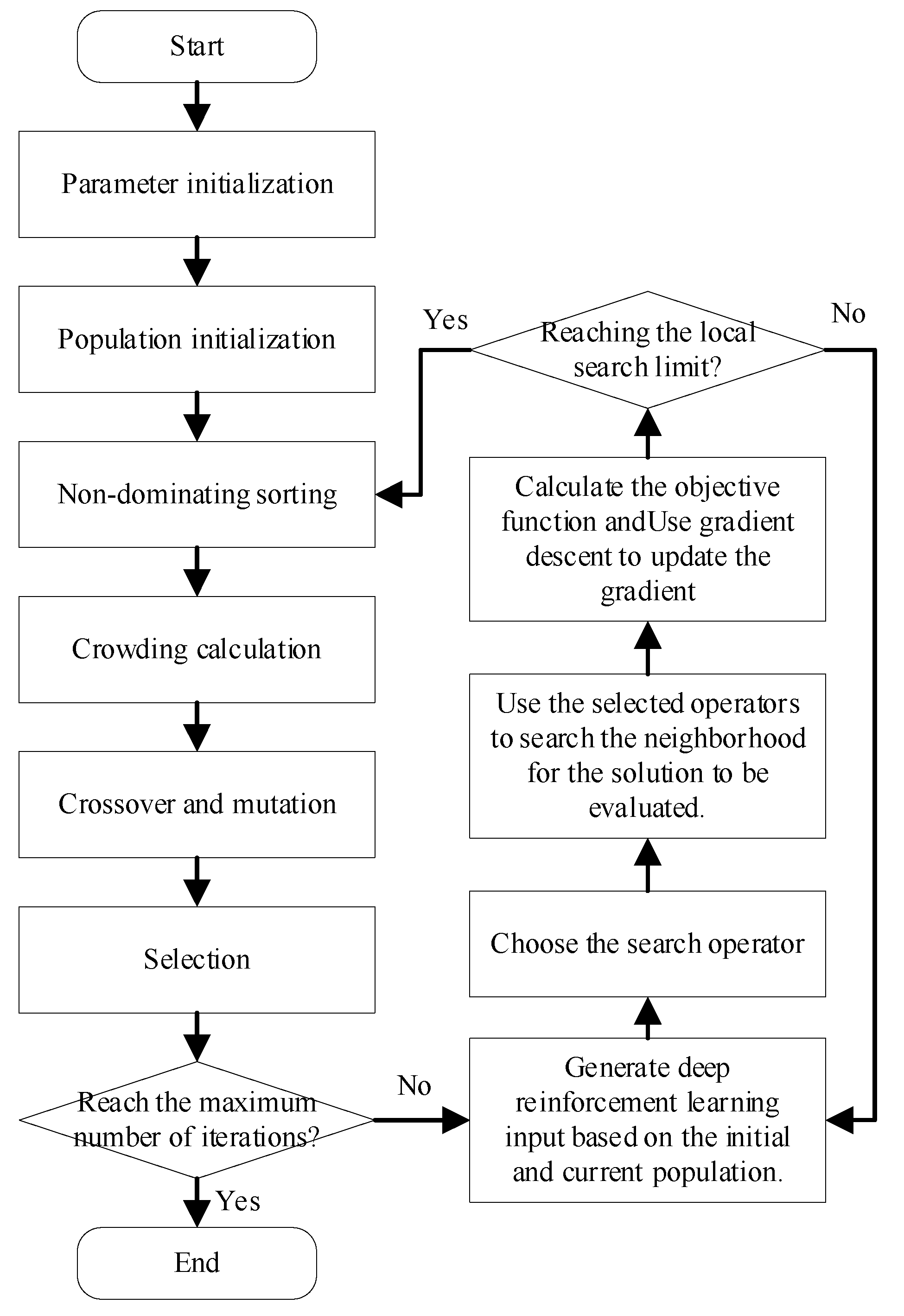
To address these challenges, we introduce a deep reinforcement learning-driven variable neighborhood search (VNS) operator. Compared with conventional VNS algorithms, our proposed operator achieves superior performance because it intelligently selects neighborhood search operators on the basis of multiple types of information collected during the iterative process. Figure 2 presents the solution framework of the enhanced NSGA-II algorithm incorporating deep reinforcement learning. The left side of Figure 2 shows the solving process of NSGA-II, whereas the right side presents the RL-VNS operator designed in this paper. Notably, since the various operators designed in this paper do not alter the nondominated sorting and crowding distance calculations of NSGA-II, their algorithmic complexity remains [28]. Here, M is the number of objectives, and N is the population size. The following subsections detail three core components: (1) the encoding scheme, (2) variable neighborhood search operators, and (3) the deep reinforcement learning-driven operator selection mechanism. The pseudocode of the solution process is shown in Algorithm 1.
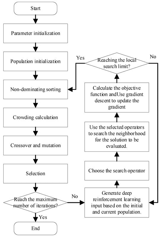
Figure 2.
Improved NSGA-II process driven by deep reinforcement learning.
| Algorithm 1 The pseudocode of improved NSGA-II process driven by deep reinforcement learning |
| Input: Demand data, processing technology data for various workpieces, and processing capability data for workstations. Output: Production scheduling scheme. 1 Initialize relevant parameters. 2 Load the deep reinforcement learning driven operator. 3 Initialize population. 4 Calculate the objective function of the initial population. 5 While the iteration limit is not reached, do: 6 Use crossover operations to search the current population. 7 Use mutation operations to search the current population. 8 Perform local search on the population using RL-VNS and update the gradient. 9 Calculate the crowding degree and perform fast non-dominated sorting. 10 Select the next generation individuals based on the elite retention strategy. 11 Output results and obtain statistical indicators. |
3.1. Encoding Scheme
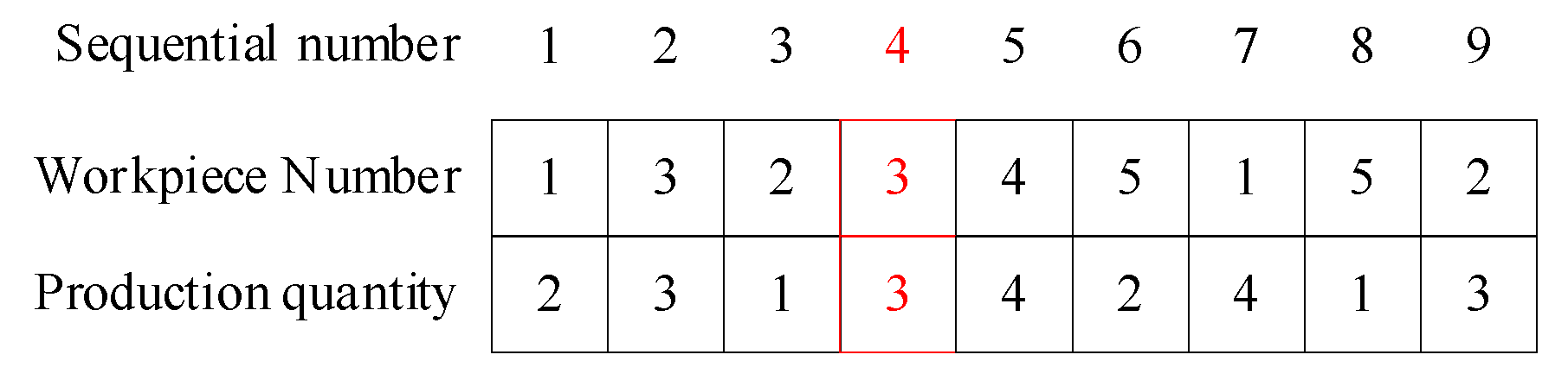
The encoding scheme selection significantly influences the computational efficiency of the enhanced NSGA-II algorithm for mixed-flow assembly line scheduling optimization. The proposed approach implements a dual-layer integer encoding strategy for chromosome representation. The first layer elements represent workpiece types corresponding to order positions, whereas the second layer elements indicate production quantities for respective order positions. Compared with single-layer chromosome encoding, this approach effectively reduces chromosome length. For example, Figure 3 presents a chromosome encoding example for a workshop that produces workpieces with five different configurations.
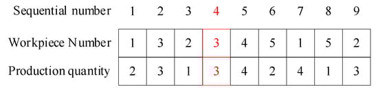
Figure 3.
Schematic diagram of chromosome coding.
As shown in Figure 3, the above chromosome indicates that the production sequence of the production plan is 1->3->2->3…, producing 2, 3, 1, 4… pieces respectively. The highlighted positions indicate overloaded positions, meaning that the quantity of workpieces being processed exceeds the threshold, and some production tasks will have additional production time.
3.2. Variable Neighborhood Search Operators
For heuristic algorithms exhibiting limited local search capabilities, performance enhancement typically involves integrating specialized local search operators. Accordingly, this study develops an enhanced NSGA-II algorithm through the implementation of variable neighborhood search operators to improve local search effectiveness. Specifically, we introduce six neighborhood search operators from two perspectives: production sequence and production quantity. These operators include the insertion search operator, reverse search operator, shuffling search operator, workload adjustment operator based on overload conditions, production position adjustment operator based on the satisfaction level, and production sequence merging operator.
The insertion, reverse, and shuffling search operators aim to identify superior production schemes by adjusting production sequences and quantities. The algorithm operates in two phases: (1) identification of search points across production cycles, followed by (2) generation of new solutions through the application of insertion, reversal, or shuffling operations. These operators implement a variable neighborhood search strategy, progressively expanding from smaller to larger search spaces. The above ideas are reflected in the first to third parts of Figure 4.
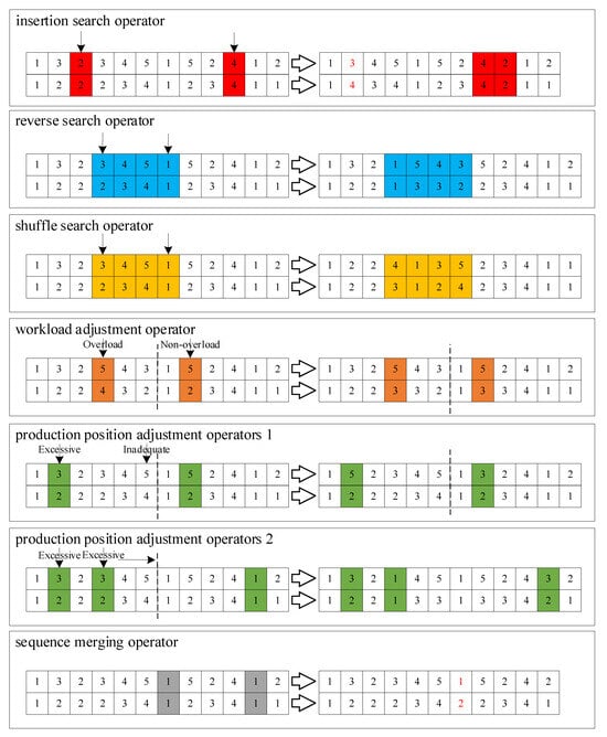
Figure 4.
Schematic diagram of local search operators.
The workload adjustment operator, designed based on overload conditions, modifies production tasks in response to the overload status of workstations. The implementation proceeds as follows: (1) randomly select an overloaded position in the current solution; (2) identify potential positions capable of transferring the entire overloaded quantity; (3) if found, transfer the overload; otherwise, partially transfer the workload until reaching the position’s capacity limit. The above idea is reflected in the fourth part of Figure 4.
Two production position adjustment operators (Operator 1 and Operator 2) were developed based on satisfaction level criteria. While both operators modify production sequences and quantities in response to delivery deviations across cycles, they employ distinct strategies: Operator 1 reallocates production by decreasing one workpiece’s quantity to increase another's, whereas Operator 2 achieves balance by redistributing specific workpieces’ production quantities across cycles. The specific mechanisms are as follows:
- Operator 1: (1) randomly select a production cycle with surplus production; (2) identify workpieces with production deficits in subsequent cycles; (3) swap their production positions.
- Operator 2: (1) Identify workpieces with surplus production; (2) locate cycles where the same workpiece shows production deficits; (3) exchange positions with other workpieces having production surplus in those cycles.
The above idea is reflected in the fifth and sixth parts of Figure 4.
The production sequence merging operator combines production quantities of the same workpiece across different positions. The procedure includes (1) randomly selecting a nonoverloaded position; (2) identifying merge-compatible positions that will not cause overload after merging; and (3) randomly selecting and merging with a compatible position. The above idea is reflected in the final part of Figure 4.
Figure 4 demonstrates the VNS operator solution process, with production positions and quantities in red font indicating merged encoding results. Unlike fixed-neighborhood local search operators, VNS employs multiple neighborhood structures. Since solutions optimal within a single neighborhood may not represent global optima, the VNS algorithm enhances search capability through diverse neighborhood exploration. This approach increases the probability of discovering superior solutions while improving overall algorithmic performance.
3.3. Deep-Reinforcement Learning-Driven Operator
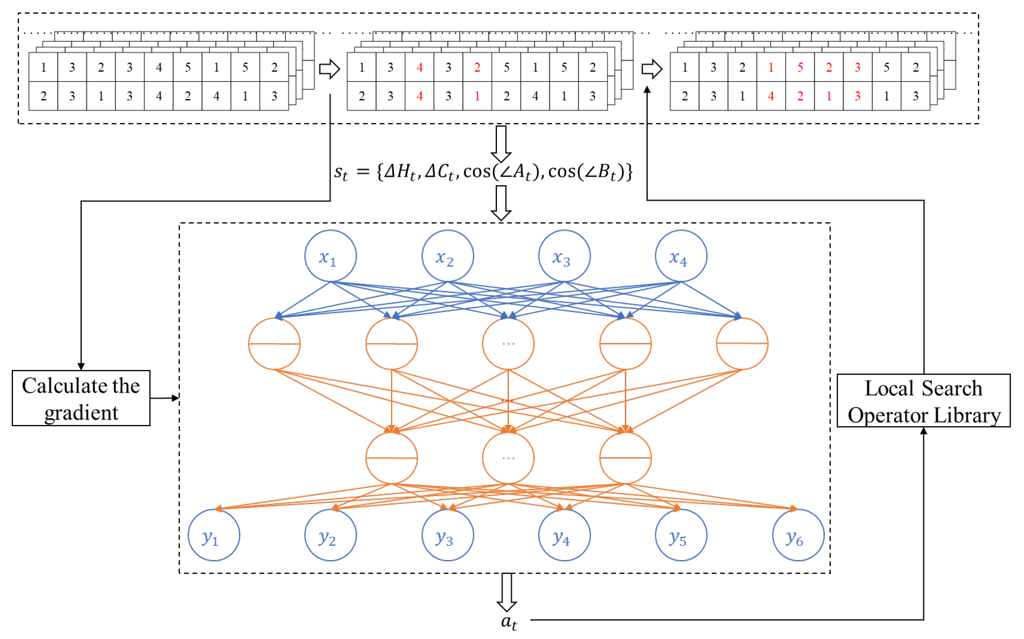
Previous research has extensively explored heuristic algorithm improvements. However, growing problem complexity and incomplete understanding of problem characteristics make heuristic design increasingly challenging [26]. Reinforcement learning offers potential solutions through environment-state-based action selection, though traditional Q-table implementations face limitations in terms of environmental definition and action space handling. Deep reinforcement learning overcomes these constraints by employing neural networks to support continuous environment representations. Building on these advances, this study develops a deep reinforcement learning-driven operator to enhance heuristic algorithms. The proposed operator dynamically collects and analyzes information about both search objects and population states during iterations, using these insights to intelligently select search operators. A schematic diagram of this approach is shown in Figure 5. The deep reinforcement learning-driven operator first obtains the network input on the basis of the population information of the current search target and then acquires the action values of each local search operator through forward propagation. A roulette wheel decision-making process is used to select the search operator on the basis of the current action values. The selected search operator is used to obtain a new population. Finally, on the basis of this new population, the effectiveness of the previous search operator is evaluated, and the gradient of the neural network is updated.
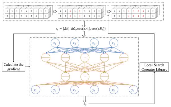
Figure 5.
Diagram of the operator driven by deep reinforcement learning.
In the deep reinforcement learning-driven operator in this study, the state space is defined via two key information types during iterations: (1) population diversity metrics (hypervolume change percentage and crowding distance change percentage from the previous action), and (2) the current search object’s objective function information. Specifically, the environmental components are as follows:
where represents the percentage change in hypervolume after the previous action, and where denotes the percentage change in the population crowding distance after the previous action. The hypervolume serves as a performance metric for multi-objective optimization algorithms and quantifies the volume of space enclosed between the optimal solution set and a reference point. The calculation formulas for hypervolume (), , and are as follows:
where represents the number of optimal solutions at time , and where indicates the volume of space enclosed between the -th solution and the reference point.
Furthermore, to characterize the relative positional relationship of a solution within the Pareto front, this study employs and to define the deep reinforcement learning state. Specifically, represents the angle formed between the search target at time t and the two extreme solutions of the optimal Pareto front before the search initiation, whereas denotes the angle formed between the search target at time t and the two extreme solutions of the current optimal Pareto front. and correspond to the cosine values of these angles.
In the deep reinforcement learning operator, the action () is defined as the selection of neighborhood search operators: . When the selected search operator yields improvements at time t, a reward () is assigned; otherwise, . Upon completing the search, the neural network weights and biases in the deep reinforcement learning operator are updated accordingly. The pseudocode for the deep reinforcement learning-driven local search operator is presented as Algorithm 2:
| Algorithm 2 The pseudocode of deep reinforcement learning-driven local search operator |
| Input: Population to be searched, deep reinforcement learning agent Output: Population after search 1 While the search task for all search objectives is not completed, do: 2 if the number of iterations < the upper limit of iterations, do: 3 Update 4 Calculate the return values of various actions under by the deep reinforcement learning operator. 5 Select the corresponding local search operator for local search based on the return values. 6 Check if the new population has improvements? Determine the reward value . 7 Determine . 8 Use to update the gradient of deep reinforcement learning. |
4. Simulation Experiments
4.1. Test preparation and parameter settings
The coding was implemented via MATLAB 2022b. The experimental environment for the simulation tests was configured as follows: CPU: 13600KF (@3.5 GHz), RAM: DDR4 32GB 4000 MHz, Hard Disk: ZHITAI Tiplus5000 2TB. The parameter settings were as follows: maximum number of iterations: 200, local search attempts: 20, population size: 20, number of hidden layers: 3, number of neurons in the hidden layers: , number of output layers: , Discount Factor: , learning rate: and activation functions: .
4.2. Algorithm Comparison Experiments
The case study data for this comparative experiment comes from the mixed-flow assembly line of BYD electric vehicles located in the Yuhua District of Changsha City, Hunan Province, China, which is responsible for the production tasks of 11 different models. Specifically, this article performs comparative experiments using 7 cases, with the experimental scenarios covered by each case shown in Table 3 below.
Table 3.
Comparison of the number of nondominated solutions (NNSs).
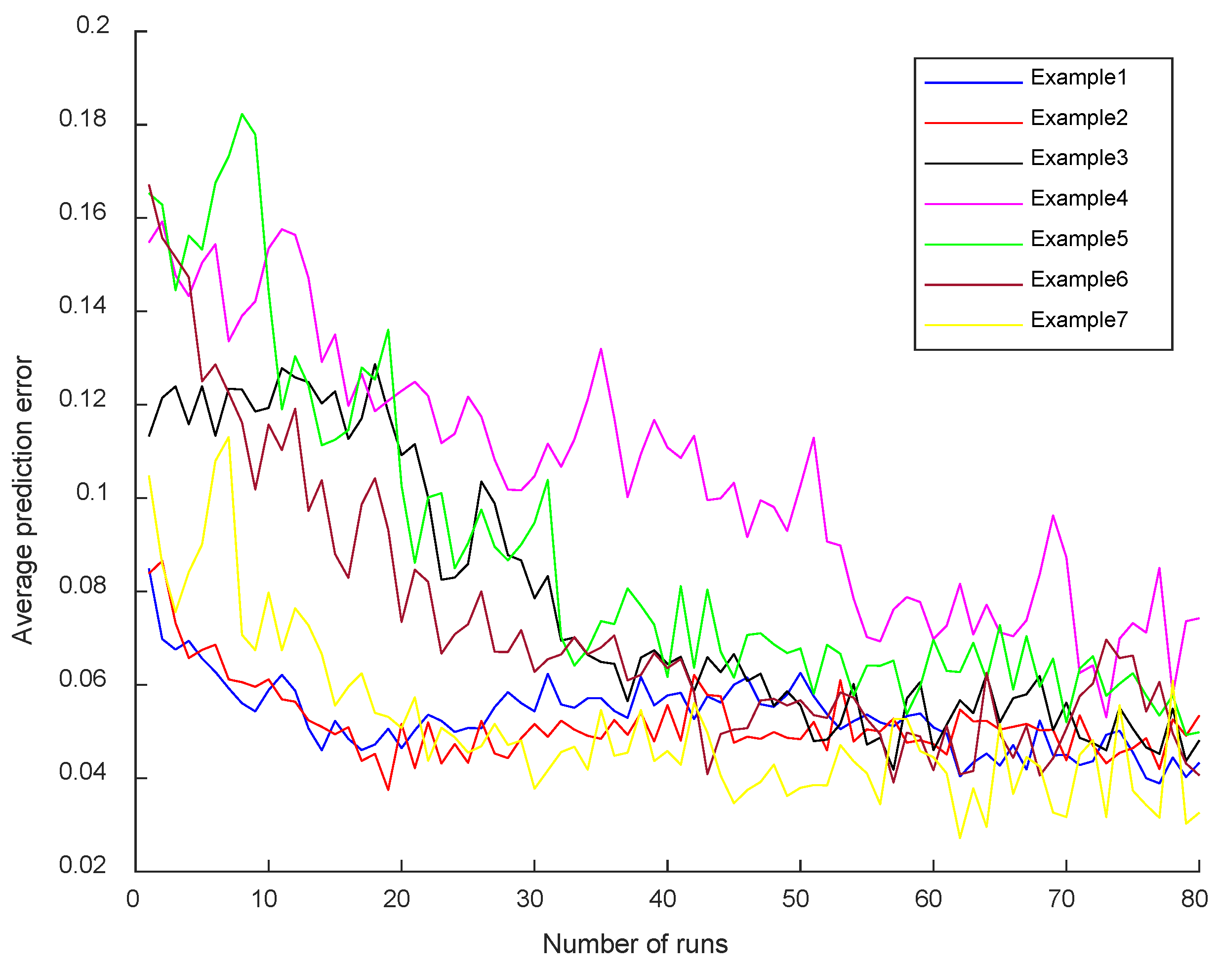
In order to verify that the deep reinforcement learning-driven operator designed in this article can effectively and accurately evaluate various states, this paper first ran the RLVNS-NSGA-II 80 times. Since the maximum number of iterations was set to 200 and the number of local searches to 30, each run of the algorithm trained the deep reinforcement learning model for times. Furthermore, this paper recorded the average estimation error of the deep reinforcement learning operator for the State Value during each run, resulting in the convergence graph of prediction errors shown in Figure 6 below.
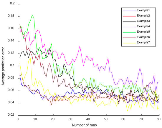
Figure 6.
Diagram of the operator driven by deep reinforcement learning.
The above prediction error diagram shows that the deep reinforcement learning-driven operator designed in this paper effectively converges to the prediction error during the learning process. This proves that the deep reinforcement learning operator gradually converges during the training process. In other words, the deep reinforcement learning operator progressively and accurately evaluates the effectiveness of each local search operator within the solution space during the iterative process, thereby guiding the algorithm to select the most appropriate operator to enhance search efficiency.
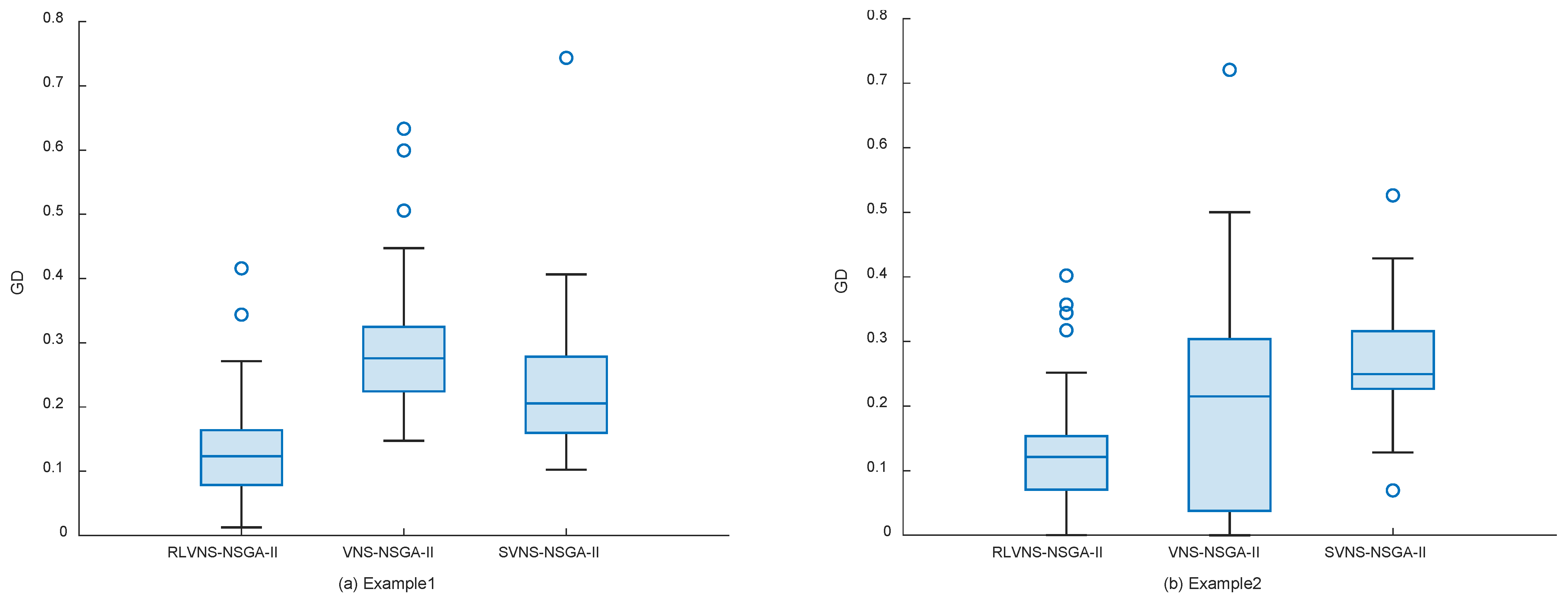
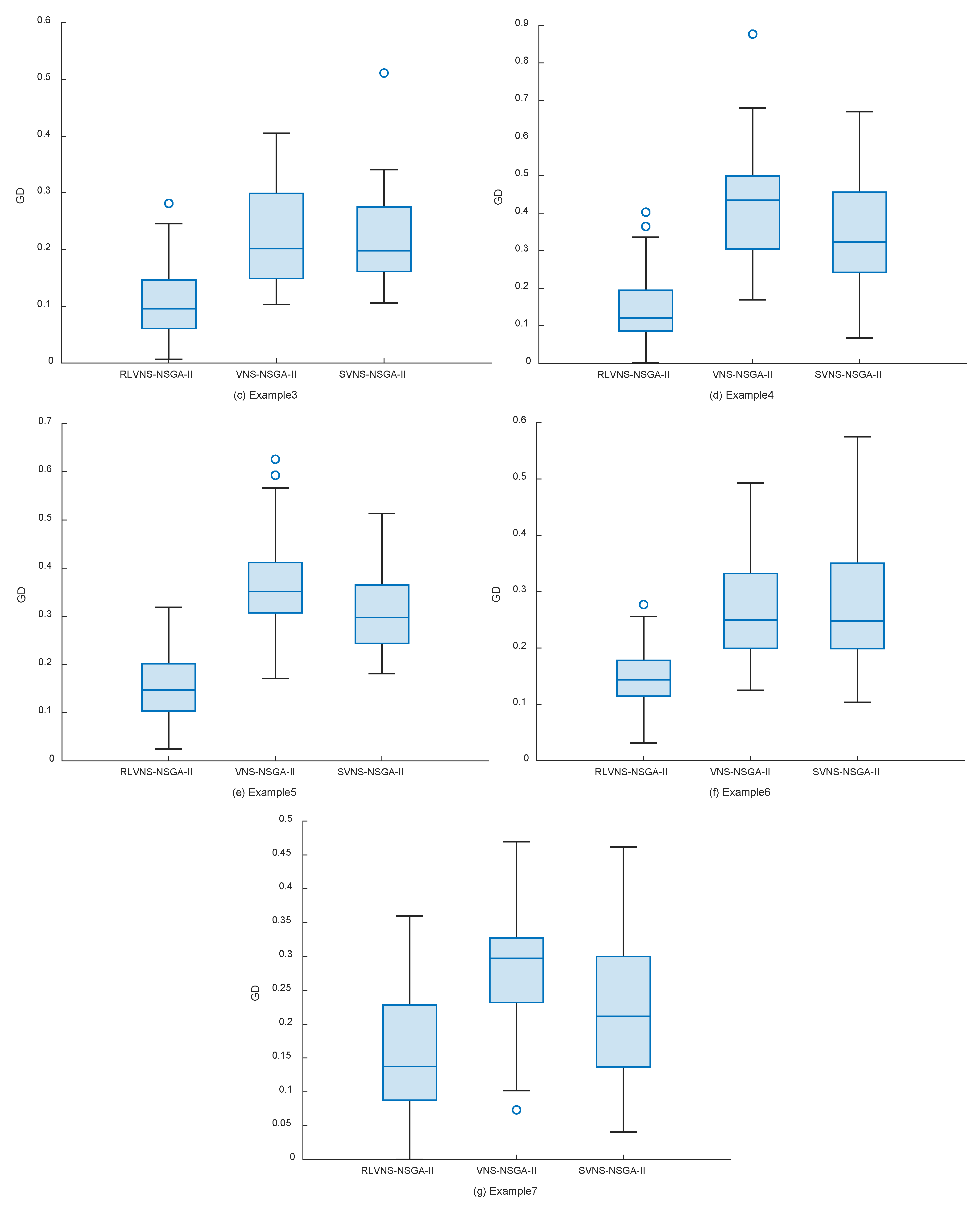
To evaluate the algorithm's performance in multi-objective optimization, the following metrics were selected: the number of nondominated solutions (), where larger values indicate more nondominated solutions in the results; the generational distance (), where smaller values indicate results closer to the Pareto front and convergence of solutions; and the hypervolume (), where larger values indicate better comprehensive performance. NSGA-II, VNS-NSGA-II improved by variable neighborhood search, and SVNS-NSGA-II with random variable neighborhood search were selected as comparison algorithms, with each algorithm running 40 times per test case. The comparison results of these metrics are shown in Table 4, Table 5 and Table 6 and Figure 7. The data for Example 1 to Example 7 are represented by (a) to (g) in Figure 7.
Table 4.
Comparison of the number of nondominated solutions (NNSs).
Table 5.
Comparison of generation distance (GD).
Table 6.
Comparison of hypervolume (HV).
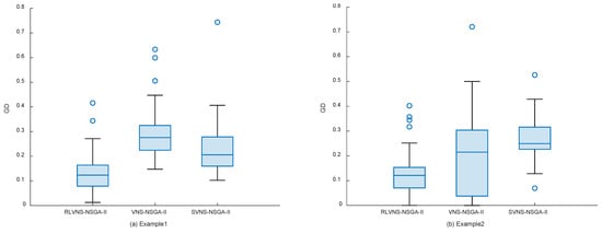
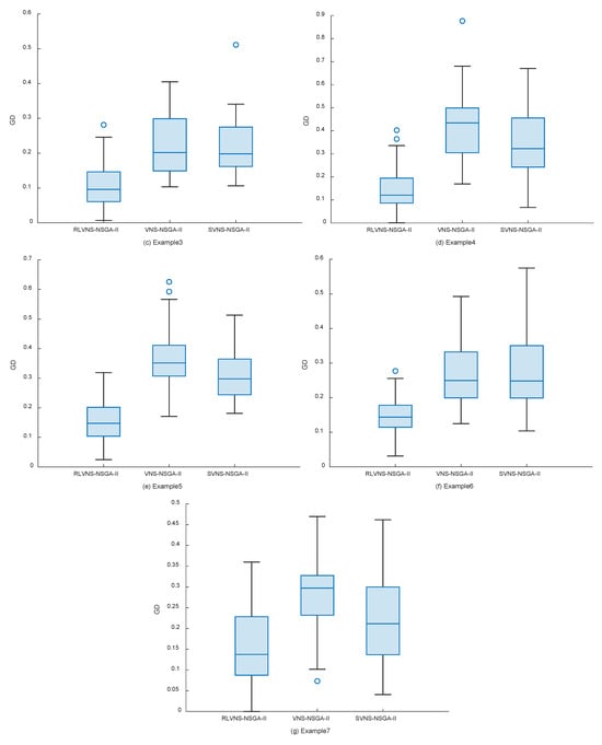
Figure 7.
Generation distance (GD) box plot.
According to Table 4, the proposed RLVNS-NSGA-II outperforms the other two algorithms in terms of the number of nondominated solutions for most test cases. This metric indicates that RLVNS-NSGA-II can obtain more nondominated solutions during optimization, thereby providing better solutions.
According to Table 5 and Figure 7, the proposed RLVNS-NSGA-II demonstrates better solving performance for most test cases: from both mean values and median distributions, RLVNS-NSGA-II’s results show smaller generational distances, and from the distributions of upper and lower quartiles, RLVNS-NSGA-II's results are all smaller than those of the other two algorithms. This metric indicates that RLVNS-NSGA-II has better convergence capability and stability than the other two algorithms.
While the above results demonstrate RLVNS-NSGA-II’s convergence capability, further evidence from Table 6 shows that the solution set obtained by this algorithm has better distribution uniformity and spread: the hypervolume of RLVNS-NSGA-II is greater than that of VNS-NSGA-II and SVNS-NSGA-II across all the examples. When VNS-NSGA-II is compared with SVNS-NSGA-II, the leading margins of hypervolume are 19.72–42.88% and 12.63–31.19%, respectively.
The aforementioned predictive errors demonstrate that the deep reinforcement learning operator can accurately assess the current state value. Furthermore, RLVNS-NSGA-II drives the operator’s decision-making process with deep reinforcement learning, whereas the other two algorithms determine the search operators on the basis of fixed or random rules. All experiments employed an identical local search operator library. The results collectively demonstrate that the proposed deep reinforcement learning-driven operator effectively guides the algorithm to: (1) leverage population diversity information, (2) utilize objective function characteristics of search objects, and (3) select appropriate search operators. This adaptive mechanism consistently improves algorithmic performance across diverse test cases.
5. Conclusion
This study develops a mixed-flow assembly line scheduling optimization model incorporating mold-changing and overload constraints, balancing production efficiency with customer satisfaction. The dual-objective formulation minimizes both additional production time and delivery deviation. To solve this model effectively, we enhance NSGA-II through: (1) integration of six neighborhood search operators, and (2) implementation of a deep reinforcement learning mechanism that guides operator selection based on population diversity and objective function information. The results demonstrate that the proposed algorithm significantly improves NSGA-II’s local search capability and outperforms both VNS-NSGA-II and SVNS-NSGA-II variants: RLVNS-NSGA-II outperforms VNS-NSGA-II and SVNS-NSGA-II with hypervolume improvements of 19.72–42.88% and 12.63–31.19%, respectively.
The practical value of this study is demonstrated in several ways. In production settings involving personalized orders, such as electric vehicle manufacturing, the proposed models and methods can support decision-making for production planning. Leveraging the characteristics of multi-objective scheduling optimization, decision-makers can generate scheduling plans that effectively balance production efficiency with customer satisfaction. Moreover, the models and methods presented in this study can be integrated into manufacturing execution systems, thereby enhancing their functionality and intelligence.
However, this study has several limitations. Future research could be enriched in the following aspects:
- Research on scheduling strategies considering inventory constraints in line-side warehouses in mixed-flow assembly scenarios is conducted.
- A bilevel programming model considering AGV routing in mixed-flow assembly scenarios is established, and scheduling strategies are studied.
Author Contributions
Conceptualization, B.Y. and T.R.; methodology, B.Y.; software, B.Y.; validation, B.Y., J.C. and T.R.; formal analysis, J.C.; investigation, X.X.; resources, B.Y., J.C., and X.X.; data curation, B.Y. and S.L.; writing—original draft preparation, B.Y. and T.R.; writing—review and editing, B.Y. and T.R.; visualization, B.Y. and J.C.; supervision, S.L. and T.R.; project administration, T.R. All authors have read and agreed to the published version of the manuscript.
Funding
This work was supported by the National Social Science Fund of China [22BJL114].
Data Availability Statement
The original contributions presented in this study are included in the article. Further inquiries can be directed to the corresponding author.
Acknowledgments
The authors would like to thank the anonymous reviewers and the editor for their positive comments.
Conflicts of Interest
The authors declare no conflicts of interest.
Abbreviations
The following abbreviations are used in this manuscript:
| DRL | deep reinforcement learning |
| NP-hard | non-deterministic polynomial |
| NSGA-II | non-dominated sorting genetic algorithm II |
| VNS | variable neighborhood search |
| HV | Hypervolume |
| GD | Generation Distance |
| IGD | Inverse Generation Distance |
| NNS | number of non-dominated solutions |
References
- Zhang, Q.B.; Si, H.Q.; Qin, J.Y.; Duan, J.G.; Zhou, Y.; Shi, H.X.; Nie, L. Double Deep Q-Network-Based Solution to a Dynamic, Energy-Efficient Hybrid Flow Shop Scheduling System with the Transport Process. Systems 2025, 13, 170. [Google Scholar] [CrossRef]
- Li, R.; Wang, L.; Gong, W.Y.; Chen, J.F.; Pan, Z.x.; Wu, Y.T.; Yu, Y. Evolutionary computation and reinforcement learning integrated algorithm for distributed heterogeneous flowshop scheduling. Eng. Appl. Artif. Intell. 2024, 135, 108775. [Google Scholar] [CrossRef]
- Zhou, F.S.; Hu, R.; Qian, B.; Shang, Q.X.; Yang, Y.Y.; Yang, J.B. Spatial decomposition-based iterative greedy algorithm for the multi-resource constrained re-entrant hybrid flow shop scheduling problem in semiconductor wafer fabrication. Comput. Ind. Eng. 2025, 208, 111330. [Google Scholar] [CrossRef]
- Wang, Y.; Ma, H.S.; Yang, J.H.; Wang, K.S. Industry 4.0: A way from mass customization to mass personalization production. Adv. Manuf. 2017, 5, 311–320. [Google Scholar] [CrossRef]
- Wu, Y.T.; Wang, L.; Li, R.; Xu, Y.X.; Zheng, J. A learning-based dual-population optimization algorithm for hybrid seru system scheduling with assembly. Swarm Evol. Comput. 2025, 94, 101901. [Google Scholar] [CrossRef]
- Shen, Z.Y.; Tang, Q.; Huang, T.; Xiong, T.Y. Solution of multistage flow shop scheduling model for leveling production. Comput. Integr. Manuf. Syst. 2019, 25, 2743–2752. [Google Scholar]
- Zhang, T.R.; Wang, Y.K.; Xie, W.; Xu, J.N.; Wang, R.L. Improved backtracking search algorithm oriented the problem of mixed flow production line sequencing. Modul. Mach. Tool Autom. Manuf. Tech. 2021, 8, 44–47+51. [Google Scholar]
- Su, Z.S.; Deng, C.; Chiong, R.; Jiang, S.L.; Zhang, K. Hybrid flow shop scheduling with continuous processing and resource threshold constraints: A case of steel plant. Expert Syst. Appl. 2025, 284, 127247. [Google Scholar] [CrossRef]
- Wang, H.; Sheng, B.Y.; Lu, X.C.; Fu, G.C.; Luo, P.P. Task package division method for the integrated scheduling framework of mixed model car-sequencing problem. Comput. Ind. Eng. 2022, 169, 108144. [Google Scholar] [CrossRef]
- Guan, L.; Wang, Y.L.; Tan, X.J.; Liu, C.L.; Gui, W.H. Machine scheduling optimization via multi-strategy information-aware genetic algorithm in steelmaking continuous casting industrial process. Control Eng. Pract. 2025, 164, 106404. [Google Scholar] [CrossRef]
- Laili, Y.J.; Peng, C.; Chen, Z.L.; Ye, F.; Zhang, L. Concurrent local search for process planning and scheduling in the industrial Internet-of-Things environment. J. Ind. Inf. Integr. 2022, 28, 100364. [Google Scholar] [CrossRef]
- Zhang, Y.H.; Hu, X.F.; Cao, X.F.; Wu, C.X. An efficient hybrid integer and categorical particle swarm optimization algorithm for the multi-mode multi-project inverse scheduling problem in turbine assembly workshop. Comput. Ind. Eng. 2022, 169, 108148. [Google Scholar] [CrossRef]
- Liu, G.Q.; Xi, H.; Wang, Y.; Wang, Z.Y. Optimization of mixed-model automobile assembly line sequencing problem based on improved genetic algorithm. Comput. Appl. Softw. 2021, 38, 78–83+137. [Google Scholar]
- Geng, K.F.; Ye, C.M. Joint scheduling of machine and AGVs in green hybrid flow shop with missing operations. Control Decis. 2022, 37, 2723–2732. [Google Scholar]
- Wu, X.L.; Cao, Z. Re-entrant hybrid flow shop scheduling problem with continuous batch processing machines. Comput. Integr. Manuf. Syst. 2022, 28, 3365–3378. [Google Scholar]
- Wallrath, R.; Zondervan, E.; Franke, M.B. Modified benders-DES algorithm for real-world flow shop and job shop scheduling problems. Comput. Chem. Eng. 2025, 202, 109221. [Google Scholar] [CrossRef]
- Gao, Q.L.; Liu, J.H.; Li, H.T.; Zhuang, C.B.; Liu, Z.W. Digital twin-driven dynamic scheduling for the assembly workshop of complex products with workers allocation. Rob. Comput. Integr. Manuf. 2024, 89, 102786. [Google Scholar] [CrossRef]
- Ding, X.J.; Gong, Z.C.; Yang, Y.P.; Shi, X.; Peng, Z.K.; Cao, X.B.; Hu, S.T. Modeling and scheduling a triply-constrained flow shop in biomanufacturing systems. J. Manuf. Syst. 2024, 76, 333–350. [Google Scholar] [CrossRef]
- Wang, L.; Pan, Z.X.; Wang, J.J. A review of reinforcement learning based intelligent optimization for manufacturing scheduling. Complex Syst. Model. Simul. 2021, 1, 257–270. [Google Scholar] [CrossRef]
- Karimi-Mamaghan, M.; Mohammadi, M.; Pasdeloup, B.; Meyer, P. Learning to select operators in meta-heuristics: An integration of Q-learning into the iterated greedy algorithm for the permutation flowshop scheduling problem. Eur. J. Oper. Res. 2023, 304, 1296–1330. [Google Scholar] [CrossRef]
- Leng, J.W.; Guo, J.W.; Zhang, H.; Xu, K.L.; Qiao, Y.; Zheng, P.; Shen, W.M. Dual deep reinforcement learning agents-based integrated order acceptance and scheduling of mass individualized prototyping. J. Clean. Prod. 2023, 427, 139249. [Google Scholar] [CrossRef]
- Yüksel, D.; Kandiller, L.; Taşgetiren, M.F. Q-learning guided algorithms for bi-criteria minimization of total flow time and makespan in no-wait permutation flowshops. Swarm Evol. Comput. 2024, 89, 101617. [Google Scholar] [CrossRef]
- Li, Z.; Wang, Y.T.; Han, Y.Y.; Gao, K.Z.; Li, J.Q. Q-Learning-Driven Accelerated Iterated Greedy Algorithm for Multi-Scenario Group Scheduling in Distributed Blocking Flowshops. Knowl.-Based Syst. 2025, 317, 113424. [Google Scholar] [CrossRef]
- Li, W.; Liang, P.; Sun, B.; Sun, Y.F.; Huang, Y. Reinforcement learning-based particle swarm optimization with neighborhood differential mutation strategy. Swarm Evol. Comput. 2023, 78, 101274. [Google Scholar] [CrossRef]
- Ding, L.S.; Luo, D.; Mudassar, R.; Yue, L.; Meng, L.L. A novel deep self-learning method for flexible job-shop scheduling problems with multiplicity: Deep reinforcement learning assisted the fluid master-apprentice evolutionary algorithm. Swarm Evol. Comput. 2025, 94, 101907. [Google Scholar] [CrossRef]
- Zheng, X.; Chen, Z. An improved deep Q-learning algorithm for a trade-off between energy consumption and productivity in batch scheduling. Comput. Ind. Eng. 2024, 188, 109925. [Google Scholar] [CrossRef]
- Yuan, M.H.; Ye, Y.; Huang, H.Y.; Zhang, Z.; Pei, F.Q.; Gu, W.B. Multi-objective energy-efficient scheduling of distributed heterogeneous hybrid flow shops via multi-agent double deep Q-Network. Swarm Evol. Comput. 2025, 98, 102076. [Google Scholar] [CrossRef]
- Deb, K.; Pratap, A.; Agarwal, S.; Meyarivan, T. A fast and elitist multiobjective genetic algorithm: NSGA-II. IEEE Trans. Evol. Comput. 2002, 6, 182–197. [Google Scholar] [CrossRef]

Disclaimer/Publisher’s Note: The statements, opinions and data contained in all publications are solely those of the individual author(s) and contributor(s) and not of MDPI and/or the editor(s). MDPI and/or the editor(s) disclaim responsibility for any injury to people or property resulting from any ideas, methods, instructions or products referred to in the content. |
© 2025 by the authors. Licensee MDPI, Basel, Switzerland. This article is an open access article distributed under the terms and conditions of the Creative Commons Attribution (CC BY) license (https://creativecommons.org/licenses/by/4.0/).