Machine Learning-Based Prediction of Resilience in Green Agricultural Supply Chains: Influencing Factors Analysis and Model Construction

Abstract

Exploring the action mechanisms and enhancement pathways of the resilience of agricultural product green supply chains is conducive to strengthening the system’s risk resistance capacity and providing decision support for achieving the “dual carbon” goals. Based on theories such as dynamic capability theory and complex adaptive systems, this paper constructs a resilience framework covering the three stages of “steady-state maintenance–dynamic adjustment–continuous evolution” from both single and multiple perspectives. Combined with 768 units of multi-agent questionnaire data, it adopts Structural Equation Modeling (SEM) and fuzzy-set Qualitative Comparative Analysis (fsQCA) to analyze the influencing factors of resilience and reveal the nonlinear mechanisms of resilience formation. Secondly, by integrating configurational analysis with machine learning, it innovatively constructs a resilience level prediction model based on fsQCA-XGBoost. The research findings are as follows: (1) fsQCA identifies a total of four high-resilience pathways, verifying the core proposition of “multiple conjunctural causality” in complex adaptive system theory; (2) compared with single algorithms such as Random Forest, Decision Tree, AdaBoost, ExtraTrees, and XGBoost, the fsQCA-XGBoost prediction method proposed in this paper achieves an optimization of 66% and over 150% in recall rate and positive sample identification, respectively. It reduces false negative risk omission by 50% and improves the ability to capture high-risk samples by three times, which verifies the feasibility and applicability of the fsQCA-XGBoost prediction method in the field of resilience prediction for agricultural product green supply chains. This research provides a risk prevention and control paradigm with both theoretical explanatory power and practical operability for agricultural product green supply chains, and promotes collaborative realization of the “carbon reduction–supply stability–efficiency improvement” goals, transforming them from policy vision to operational reality.

1. Introduction

In the context of profound transformations in global climate governance systems and accelerated transitions to a low-carbon economy, the green agricultural supply chain system serves as a critical bridge between agricultural production and consumer demand strategies. Its ecological efficiency optimization has become a key variable influencing food security and the progress of “dual carbon” strategies, making energy conservation and emissions reduction a focal point in China’s current agenda [1]. World Bank data indicate that greenhouse gas emissions from supply chain activities account for over 40% of total emissions in the global food supply chain, significantly surpassing the average levels in manufacturing supply chains. According to the State Council’s “14th Five-Year Plan for Cold Chain Supply Chain Development,” it is mandated that carbon intensity in cold chain supply chains be reduced by 40% by 2025. This implies that while ensuring the fresh produce supply for nearly 900 million urban residents, the agricultural supply chain system must achieve deep decarbonization, addressing the complex challenge of balancing “carbon reduction–stable supply–efficiency enhancement.” Research on green supply chain systems has thus entered a critical phase focused on multi-objective collaborative optimization [2,3,4]. The green agricultural supply chain refers to the process of optimizing supply chain resources, adopting advanced technologies, and implementing efficient supply chain activities to reduce the environmental impacts caused by agricultural supply chain operations [5]. It possesses characteristics such as ecological sensitivity, policy orientation, and technological dependency [6,7,8]. Traditional research often simplifies the resilience of green supply chains into issues of technological upgrades or policy compliance, neglecting the synergistic effects among policies, technologies, and markets. This oversight leads to a single-factor dependency trap when systems encounter sudden disturbances, potentially causing carbon emission rebounds. Therefore, constructing a high-resilience green agricultural supply chain system at low cost and high efficiency—ensuring normal product supply while maintaining low-carbon operations—has become a core issue within China’s ecological protection system. Consequently, investigating how to enhance the resilience of green supply chain systems through supply chain management, revealing the mechanisms driving resilience formation driven by multiple factors, and developing dynamic early-warning decision support tools are crucial. However, research on the resilience of green supply chains for agricultural products is still in its infancy. Existing studies are mainly qualitative, with few empirical analyses based on real-world enterprise survey data. Most studies only explore the impact of individual or small numbers of factors on supply chain resilience. Moreover, they often use a single research method, ignoring the combined effects of multiple factors and empirical research on different factor combinations. Additionally, there is a lack of utilization of emerging tools, such as machine learning, for predicting resilience levels.

This study analyzes key influencing factors of the resilience of green agricultural supply chains through a three-stage observation framework covering stability maintenance, dynamic adaptation, and continuous evolution. Based on mixed cross-sectional samples involving government, enterprises, consumers, and producers derived from 768 multi-stakeholder questionnaire responses, the research first employs Structural Equation Modeling (SEM) to identify the impact of individual factors on resilience and constructs predictive models using traditional machine learning algorithms. Secondly, it utilizes fuzzy-set Qualitative Comparative Analysis (fsQCA) to recognize configurational effects of multiple factor combinations and innovatively develops a resilience prediction model based on fsQCA-XGBoost. The findings reveal that fsQCA identifies equivalent pathways for enhancing resilience; XGBoost transforms configurational paths into dynamic risk warning features, achieving a closed loop from “causal diagnosis” to “risk intervention”. Finally, the paper provides deployable intelligent decision anchors for regional differentiated governance.

This study aims to answer the following questions: (1) Which technological, institutional, and market factors significantly influence the resilience of green supply chains? (2) How do these factors achieve the goals of “carbon reduction–stable supply–efficiency enhancement” through configuration? (3) How can governments and enterprises select optimal intervention strategies based on dynamic resilience changes?

2. Literature Review and Theoretical Framework

2.1. Conceptualization of Resilience

The term “resilience” originally emerged from disciplines such as physics, psychology, ecology, and economics [9,10]. Scholars generally define it as the capacity of a system to maintain functionality in the face of disruptions. In the field of supply chain management, resilience research has primarily focused on inventory redundancy and transportation path optimization [11], with limited integration of green or sustainability considerations. In contrast, studies on green agricultural supply chains have emphasized technological innovation and circular practices, yet lack a quantifiable framework for assessing resilience. Although the concept of “carbon lock-in breaking capacity” provides a theoretical foundation for green supply chains [12], its application remains constrained in practical contexts. First, it does not adequately quantify environmental resilience. Second, it overlooks the interaction between policy regulation and technology diffusion. To address these gaps, some scholars have proposed methodological insights for sustainable supply chains by emphasizing emissions control, efficiency enhancement, and the importance of coping with uncertainty [13], which offer valuable references for resilience research in green supply chains.

Based on this, this paper proposes an integrated definition of the resilience of China’s agricultural green supply chain system: under the guidance of policies, governments, enterprises, and large-scale producers achieve dynamic equilibrium of low-carbon operations, stable supply, and efficiency improvement through technological innovations such as low-carbon supply chains and low-carbon packaging, in collaboration with market mechanisms, throughout the cycle of transportation, warehousing, processing, and distribution. This simultaneously enhances the system’s adaptive capacity to environmental changes and market fluctuations. The system’s stakeholder structure includes governments, enterprises, producers, and consumers, emphasizing the dynamic balance of carbon reduction, supply stability, and efficiency improvement, with adaptive capacity to internal and external changes. This definition aligns with the research’s questionnaire survey methodology, demonstrating the following: (1) goal synergy, translating the triple constraints of “carbon reduction–supply stability–efficiency improvement” into quantifiable operational targets; (2) process dynamics, breaking through the traditional “resistance–recovery” dichotomy to emphasize stepwise transitions in the system’s green evolution and operational processes; (3) path configurationality, revealing the synergistic effects of multi-factor and multi-stakeholder interactions, providing a theoretical anchor for the subsequent SEM-fsQCA analysis.

2.2. Risks and Challenges in Green Supply Chains

Resilience essentially represents a set of capabilities through which a system maintains dynamic equilibrium amid multidimensional risks such as policy constraints, technological bottlenecks, market fluctuations, and natural disturbances. This capability not only manifests as the steady-state maintenance capacity to withstand shocks but also embodies the dynamic adaptation capability to identify risks and the sustained evolution capability to break through bottlenecks. Currently, the agricultural green supply chain is facing transformation challenges under the interwoven superposition of the above-mentioned risks.

1. Policy Constraints and Compliance Costs. The policy framework for achieving the dual carbon goals imposes stringent carbon emission constraints on agricultural supply chains. However, there is a significant tension between the rigid enforcement of policies and the gradual nature of industry transformation. For instance, the cost of low-carbon technologies in agricultural supply chains is prohibitively high—hydrogen-powered refrigerated trucks cost 2.3 times more than traditional diesel vehicles (IEA data). Policies tend to favor large-scale supply chain enterprises, leaving small and medium-sized enterprises (SMEs) facing the dilemma of “compliance equals loss” during technological upgrades [14]. Additional challenges include the complexity of embedded emissions accounting [15], third-party certifications [16], ambiguous boundaries of carbon emissions [17], and the immaturity of carbon trading markets [18]. These issues are further exacerbated in cross-border supply chain scenarios, where companies often incur an additional 12–15% in green certification costs to meet international standards [19].

2. Insufficient Technological Maturity and Extended Return on Investment Periods. The effectiveness of green supply chain technologies directly determines the feasibility of low-carbon transitions. However, bottlenecks in core technology maturity hinder the synergy among the three objectives. In warehousing, photovoltaic cold storage requires over-provisioning due to battery technology barriers to ensure stable energy supply [20]. The application costs of Internet of Things (IoT) technologies in supply chains are excessively high [21]. In packaging, biodegradable materials cost 2–3 times more than conventional materials and lack sufficient mechanical strength and water resistance, making them difficult to fully replace [22]. Recycling rates for green packaging remain below 30%, with incomplete coverage of sorting and processing facilities. Paper-based packaging contaminated with agricultural residues often ends up in landfills or incineration, negating low-carbon benefits [23]. In transportation, hydrogen storage faces challenges such as boil-off losses and limitations in materials and catalysts [24]. Hydrogen vehicles have lower range capabilities, leading companies to retain fuel vehicles as backups, resulting in a vicious cycle of “high investment–low utilization–carbon emission rebound.” It is evident that optimizing single technical parameters alone cannot break the systemic lock-in effect; instead, it requires collaborative innovation across multiple parties to reconstruct the supply chain network. This approach, however, increases initial investment costs for participating entities and extends the payback period.

3. Market Acceptance Lag and Green Premium Dilemma. The cost changes associated with green supply chain transitions are often passed on to consumers through price transmission mechanisms, making consumers’ willingness to pay (WTP) a critical variable. Research indicates that consumers are reluctant to accept higher product premiums [25], thus favoring lower-priced non-green products [26]. However, the premium generated by green certification can only cover 40% of the increased costs for farmers [27,28]. This results in dual cost dissipation: on the one hand, companies incur increased costs to achieve green supply chain transformation; on the other hand, market share may shrink due to price sensitivity. A deeper contradiction lies in the divergence between market preferences and policy objectives: while governments encourage enterprises to pursue low-carbon transitions, end consumers prioritize delivery speed and quality, driven by self-interest rather than altruistic motives [25].

4. Cross-Boundary Transmission Effects of Natural–Social Systems. Traditional risks also significantly disrupt green supply chains and amplify transition risks through energy–supply chain–consumer chain transmission. For example, high temperatures can cause cold chains to fail, and floods can interrupt transportation routes [29], resulting in additional operational costs of 20–30% for both companies and governments [30]. In North China, photovoltaic modules frequently reach temperatures above 55 °C during summer months, leading to an overall power loss of up to 20–30% of theoretical values [31]. Power shortages force governments to adjust energy dispatch strategies, such as increasing coal-fired power generation, further amplifying carbon emission intensity. Policy biases exacerbate system vulnerability. For instance, by 2023, China had established 358 hydrogen refueling stations, primarily concentrated in clusters. The cross-boundary transmission effects of natural–social systems highlight the deep-seated contradictions between tackling climate change and green supply chain upgrades.

2.3. Influencing Factors of Resilience

The core of resilience in agricultural green supply chains lies in dynamically coordinating and balancing policy guidance, technological innovation, and market mechanisms. This concept is theoretically grounded. Innovation systems theory posits that technological innovation is embedded within a complex system of diverse entities, including businesses and governments. The interaction of system elements like institutions, factors, and market demand shapes innovation’s direction and speed [32,33]. Transition management theory further suggests that transitioning sustainable socio-technical systems (e.g., green supply chains) is a long-term, nonlinear process involving multiple levels and actors. Policies guide transitions by setting visions and establishing institutional frameworks. Technological breakthroughs emerge in niches and seek scaling-up, while markets drive transitions through demand, resource allocation, and user feedback. These three elements need to co-evolve across different levels to overcome the “lock-in” effects and path dependence of existing high-carbon systems [34,35,36]. Institutional theory reveals how formal and informal rules shape the legitimacy of technology choices and the rationality of market behaviors. Changes in technological paradigms and market forces also drive adaptive adjustments in institutions [37,38]. Together, these theories indicate that policy, technology, and the market form an interdependent and co-evolving system. The effectiveness of their coordination, reflected in achieving policy goals, overcoming technological bottlenecks, and responding to market signals, is crucial for the system to maintain dynamic balance and continuous evolution under multiple risks, thus ensuring its resilience [39]. This provides the theoretical foundation for this study’s subsequent exploration of multi-stakeholder configuration effects (SEM-fsQCA).

In the current literature and existing research, scholars mainly focus on three dimensions: steady-state maintenance capability, dynamic adaptation capability, and sustained evolution capability. In terms of steady-state maintenance capability, originating from ecological resilience theory, this dimension emphasizes the system’s ability to maintain the stability of core functions after disturbances [32]. In green supply chain systems, it manifests as achieving dynamic coordination between low-carbon operations and supply through technological and management means. Firstly, it relies on redundancy [32,33,34,35,36,37,38,39,40,41], where redundant design enhances system stability and reduces sensitivity to disturbances [41], which is essential for preventing collapse [42]. Scholars argue that redundant packaging made from recyclable materials [43] and low-power redundant components can contribute to carbon reduction [44]. Secondly, it depends on real-time feedback and monitoring within the system. Based on cybernetics [42] and the “ecosystem health monitoring” framework [45,46], scholars suggest that dynamic monitoring can activate redundant equipment as needed, optimizing resource utilization [47].

In terms of dynamic adaptation capability, drawing from supply chain resilience theory, circular economy theory, and agile supply chain theory, this dimension focuses on the ability to resist disturbances and rapidly recover to a steady state through resource reorganization [48,49,50]. In green supply chain systems, it involves using management strategies to address disruptions, quickly restoring low-carbon supplies, and continuously optimizing resource use. Firstly, regarding low-carbon disturbance recovery capability, the implementation of new carbon reduction policies [51], technological changes, or market demand shifts [52] can cause fluctuations in the supply chain system. Ant colony algorithms [38] can dynamically adjust transportation, reducing carbon emission costs and improving transport efficiency [53]. Efficiency improvements lower energy dependency [54], balancing the dual goals of emission reduction and efficiency enhancement [55]. Secondly, resource circulation agility (resource recycling elasticity) is defined as “the ability to rapidly respond to changes during the recycling process, optimize resource allocation, and enhance recycling efficiency.” The core lies in shortening the resource turnover cycle and flexibly allocating resources to address unpredictable situations [56]. In the context of green supply chain systems, scholars emphasize the capabilities of resource reconfiguration [56] and resource closed-loop [5], which can be achieved through measures such as reducing the identification time of recycled products, enhancing the transparency of reverse supply chains [57], and establishing agile response mechanisms [58].

In terms of sustained evolution capability, this is the core capability for long-term low-carbon resilience in green supply chain systems, encompassing two major dimensions: collaborative innovation and institutional restructuring. Collaborative innovation originates from collaborative innovation theory, emphasizing collaboration among diverse actors to form an “open innovation ecosystem” [59]. In green supply chain systems, the core of collaboration is cross-organizational resource integration and co-creation of knowledge, grounded in shared environmental goals among diverse supply chain actors [60,61], and it also lies in bridging the gaps between policy objectives, technological feasibility, and market acceptability. Establishing joint research centers across sectors to rapidly respond to technological changes [62,63] and industrial symbiosis networks [64] are current research hotspots. Tatarczak (2020) developed an enhanced VIKOR method for logistics collaboration decision-making in intuitionistic fuzzy environments. It offers a quantitative tool for coordinating interests and allocating resources among supply chain entities [65]. Key pathways for collaboration include technology integration and benefit distribution; issues such as the incompatibility of new energy vehicles [65] and conflicts between environmental investment and returns [66] need urgent resolution; effective collaborative innovation can accelerate technology maturation and cost reduction, enhance market willingness to pay for green products, and optimize policy design through feedback, creating a virtuous cycle. Institutional restructuring is theoretically grounded in institutional change theory [67], complex adaptive systems theory [68], and policy learning theory [69], emphasizing both the learning and bargaining processes between actors and institutions, as well as “adaptive actors.” In green supply chain systems, there is a preference for a symbiotic relationship between technological collaboration and dynamic policy adjustments, guiding the supply chain system towards environmentally friendly and resource-efficient transformations. The focus of institutional restructuring is on multi-actor collaboration led by policy [5,70]. Additionally, government regulatory pressure [71] and legal enforcement [72] are also critical factors. It should be noted that the effectiveness of institutional restructuring is highly contingent on its capacity for dynamic responsiveness to technological trajectories and market feedback signals.

In summary, redundancy is intended to enhance system stability and reduce carbon emissions through technical means; real-time feedback and monitoring aim to activate redundant equipment and optimize resource utilization via dynamic monitoring technologies; low-carbon disturbance recovery capability seeks to reduce costs through technologies and respond to changes in market demand; the core of resource circulation agility lies in market response supported by technologies; collaborative innovation relies on technological innovation and institutional coordination; and institutional restructuring dynamically responds to technological trajectories and market signals. All these six factors reflect their dependence on and connection with technology, institutions, and markets. Through a synthesis of previous research, the present study has identified six key factors that influence resilience, but currently, research on the resilience of agricultural green supply chains is still plagued by several limitations. First, most existing studies adopt a single-actor perspective while neglecting multi-stakeholder coordination mechanisms, leading to long-term ignorance of configurational effects among diverse actors. Second, traditional resilience assessments lack forward-looking predictive capabilities for dynamic risk evolution, failing to quantify key dynamic fluctuations such as the stability of low-carbon operations. Third, mainstream methodologies have failed to develop quantifiable and deployable early-warning tools for risk identification. Overall, based on 768 units of questionnaire survey data, this paper systematically explores the single and combined influence effects of resilience by integrating Structural Equation Modeling (SEM) and fuzzy-set Qualitative Comparative Analysis (fsQCA), and constructs a risk prediction model by fusing machine learning methods based on configurational effects.

3. Analysis of Influencing Factors of Resilience

1. Questionnaire Design and Data Collection. Drawing on survey data, this study targeted four stakeholder groups: 106 enterprise employees, 354 consumers, 168 public officials, and 140 producers. A total of 768 questionnaires were distributed, yielding 469 valid responses, corresponding to an effective response rate of 61.07%. Invalid questionnaires were mainly due to incomplete completion (about 88%), and were not significantly related to respondents’ roles and regions. We performed independent-sample T-tests on the core characteristics (e.g., resilience levels) of samples returned early (first 30%) and late (last 30%). The results indicated no significant differences in key variables between the two groups (p-value > 0.05), suggesting that non-respondents had minimal impact on the overall representativeness. Initially, differentiated questionnaires were designed for each group; subsequently, they were integrated and optimized into a universal version (see Appendix A.1) to systematically present the measurement indicators employed in this research. Respondents were strictly restricted to enterprise managers with work experience in the agricultural product supply chain, as well as producers and consumers directly or indirectly involved in the production, circulation, and consumption of agricultural products, thereby ensuring the professionalism of the sample and the authenticity of the data.

2. Descriptive Statistics of the Sample. Through data organization and statistical analysis of the questionnaire responses, descriptive results were obtained. The sample included a relatively high proportion of agricultural enterprise employees and public officials, indicating strong representativeness, particularly in the fields of green supply chain management and policy implementation. Most enterprise staff and public officials who completed the questionnaires held middle or senior management positions in relevant departments, which to some extent ensured the reliability of the collected data. The inclusion of consumers and producers enriched the sample with perspectives from multiple stages of the agricultural product supply chain. This multi-stakeholder composition contributes to a comprehensive understanding of different stakeholders’ perceptions and roles in relation to the resilience of green agricultural supply chains. Detailed results are presented in Appendix A.2.

3. Reliability and Validity Analysis. This study employed internal consistency coefficients (Cronbach’s α) and composite reliability (CR) to assess reliability. The results showed that all variable α coefficients were above 0.7 (α for supply chain resilience = 0.883), and CR values also exceeded 0.7, indicating good scale reliability. Validity was evaluated through content validity, structural validity, convergent validity, and discriminant validity. Content validity was ensured by using an established scale and applying a “translation–back translation” procedure. Structural validity was confirmed via the KMO (Kaiser–Meyer–Olkin) measure of sampling adequacy (0.923) and Bartlett’s test of sphericity (χ² = 5200.550, p < 0.05), both indicating suitability for factor analysis. Confirmatory factor analysis further demonstrated acceptable model fit indices: χ²/df = 1.064, RMSEA = 0.012, GFI = 0.966, CFI = 0.998. Convergent validity was supported by factor loadings above 0.5, average variance extracted (AVE) greater than 0.5, and composite reliability (CR) above 0.7. Discriminant validity was verified by comparing the square root of each construct’s AVE with the absolute correlation coefficients between constructs—these values were consistently higher, confirming adequate discriminant validity (see

Table 1. Reliability and Validity Analysis of the Scale.

	FX	GB	DK	FY	CX	HF	ASCR
FX	0.757
GB	0.424 **	0.732
DK	0.409 **	0.462 **	0.799
FY	0.453 **	0.516 **	0.538 **	0.840
CX	0.390 **	0.397 **	0.370 **	0.454 **	0.740
HF	0.434 **	0.480 **	0.470 **	0.501 **	0.434 **	0.793
ASCR	0.473 **	0.525 **	0.477 **	0.550 **	0.503 **	0.537 **	0.863
Cronbach’s α	0.800	0.775	0.841	0.877	0.785	0.835	0.883
CR	0.801	0.776	0.841	0.878	0.784	0.835	0.897
Square Root of AVE	0.573	0.536	0.639	0.706	0.548	0.628	0.744

Note: ** p < 0.01; diagonal values represent average variance extracted (AVE).

).

4. Model Fit Analysis. To assess the alignment between the theoretical model and the empirical data, this study conducted a model fit test using Structural Equation Modeling (SEM) with AMOS 26.0 software. The model fit indices are presented in

Table 2. Goodness-of-Fit Indices for the Model.

Fit Index	Value	Threshold	Interpretation
CMIN/DF	1.064	1–3	Value between 1 and 3, good fit
RMR	0.019	0.05	Below threshold, excellent fit
GFI	0.966	≥0.9	Above threshold, good fit
AGFI	0.953	≥0.9	Above threshold, good fit
NFI	0.966	≥0.9	Above threshold, good fit
IFI	0.998	≥0.9	Above threshold, good fit
TLI	0.997	≥0.9	Above threshold, good fit
CFI	0.998	≥0.9	Above threshold, good fit
RMSEA	0.012	≤0.08	Below threshold, excellent fit

Note: CMIN/DF represents the ratio of chi-square to degrees of freedom; RMSEA stands for root mean square error of approximation; CFI, TLI, and IFI are fit indices, where values ≥ 0.9 generally indicate a good model fit.

: CMIN/DF = 1.064, RMSEA = 0.012, RMR = 0.019, GFI = 0.966, AGFI = 0.953, CFI = 0.998, TLI = 0.997. All indices meet or exceed the conventional criteria for model fit, indicating that the model demonstrates excellent overall goodness-of-fit.

3.1. SEM-Based Analysis of Influencing Factors

Structural Equation Modeling (SEM) is a multivariate statistical analysis technique primarily used to examine causal relationships among variables. Through path analysis and factor loading tests, SEM enables the assessment of both direct and indirect effects of system drivers. SEM allows researchers to simultaneously consider the impacts of multiple independent variables on multiple dependent variables. In this study, the structural equation model was employed to conduct a preliminary analysis of the factors influencing the resilience of green agricultural supply chains, aiming to identify the specific roles of each factor in shaping supply chain resilience. Based on the satisfactory model fit, the structural equation model was further tested using AMOS 26.0 statistical software. The resulting path analysis diagram is presented in Figure 1.

As shown in

Table 3. Hypothesis Testing Results.

Latent Variable	Path	Observed Variable	Hypothesis	Unstandardized Coefficient	Unstandardized Coefficient	Standard Error	Critical Ratio	p-Value
ASCR	←	FX	H1a	0.18	0.14 *	0.073	2.477	0.013
ASCR	←	GB	H1b	0.305	0.217 ***	0.096	3.188	0.001
ASCR	←	DK	H2a	0.061	0.056	0.063	0.968	0.333
ASCR	←	FY	H2b	0.143	0.142 *	0.064	2.248	0.025
ASCR	←	CX	H3a	0.241	0.206 ***	0.066	3.627	0.000
ASCR	←	HF	H3b	0.199	0.19 **	0.064	3.112	0.002

Note: * p < 0.05, ** p < 0.01, *** p < 0.001.

, redundancy (β = 0.14, p < 0.05), feedback capacity (β = 0.217, p < 0.01), agility (β = 0.142, p < 0.05), innovation capability (β = 0.206, p < 0.001), and reconfiguration capability (β = 0.19, p < 0.01) have significant positive effects on supply chain resilience. In contrast, recovery ability (i.e., low-carbon disturbance recovery ability) (β = 0.056, p = 0.333) does not show a significant impact on supply chain resilience. The insignificant low-carbon disturbance recovery ability may stem from the particularity of the agricultural green supply chain. Firstly, when the system is subjected to a disturbance (such as equipment failure or a sudden policy change), traditional recovery methods (such as activating diesel-powered backup cold stores or switching to high-carbon transportation routes) can quickly restore the supply, but they lead to a rebound in carbon emissions. This “recovery–increasing carbon” paradox undermines the contribution of DK to the dual goal of “decarbonization–supply stability”. Secondly, resource circulation agility (FY), as one of the core drivers of resilience, can achieve “supply stability” and “decarbonization” simultaneously through rapid resource reorganization (such as shared cold store scheduling and multimodal transportation route optimization) under sudden disturbances, thus partially substituting for the single recovery function of DK. Finally, the effectiveness of the recovery ability (DK) is highly dependent on the institutional framework (such as carbon quota flexible policies and cross-border certification mutual recognition). In the absence of institutional support, enterprises find it difficult to implement real low-carbon recovery, and therefore, it is difficult to analyze the recovery ability in isolation.

3.2. fsQCA-Based Analysis of Configurational Effects

Given the prevalent phenomenon of “multiple concurrent causal pathways” in supply chain resilience, this study adopts a configurational analysis approach combined with machine learning to model the synergistic effects. This is due to the fact that resilience may depend on a combination of multiple elements, which are interdependent and interrelated, and collectively act on resilience. Meanwhile, different combinations of elements may lead to the same outcome, and the path to achieving resilience is not unique. As a configurational analysis method, QCA can, on the basis of SEM model research, effectively handle the interactions between more than three variables. By exploring the sufficient and necessary subset relationships between antecedent conditions and outcomes, it supplements the analysis of the impact of different factor combinations on resilience from a configurational perspective. Also, existing studies have shown that the effective integration of these two methods can enhance the descriptive, predictive, and explanatory power of social science theories. Depending on the types of variables, common QCA analysis methods include three types: crisp-set Qualitative Comparative Analysis (csQCA), multi-value Qualitative Comparative Analysis (mvQCA), and fuzzy-set Qualitative Comparative Analysis (fsQCA). Among them, both csQCA and mvQCA can only handle categorical issues. By assessing the degree of membership of variables between full membership and full non-membership, fsQCA can be used to handle interval and ratio variables, enabling the QCA method to deal with continuous variables and partial membership issues. This enhances the practicality and universality of the analysis, which is why fsQCA is gradually becoming the mainstream choice for applying the QCA method. This study adopts the fsQCA analysis method to further explore the effect of multi-factor combinations on resilience.

First, fuzzy-set Qualitative Comparative Analysis (fsQCA) is employed to generate configurations that directly characterize the patterns of resilience levels formed by the interplay of multiple factors. Subsequently, signal–noise separation is conducted. Finally, asymmetric relationships are captured, thereby enhancing the accuracy of the resilience level prediction model.

(1) Data Preprocessing. Based on theoretical and empirical research, the following five variables were selected as condition variables: Redundancy (FX), Feedback Capacity (GB), Agility (FY), Innovation Capability (CX), and Reconfiguration Capability (HF). The resilience of the green agricultural supply chain was selected as the outcome variable. The data were calibrated into fuzzy-set scores ranging from 0 to 1 using fsQCA. Variable values were calculated based on the average score of corresponding questionnaire items. Calibration thresholds were set as follows: 5 (full membership), 3.001 (crossover point—slightly adjusted to capture differentiation due to system exclusion of 0.5 membership values), and 1 (full non-membership). Necessity analysis (see Appendix A.3) revealed that no single condition was a necessary factor for resilience, indicating the need for multi-factor configurational analysis.

(2) Configuration Sufficiency Analysis. A consistency threshold of 0.933 and a frequency threshold of 7 (covering 80% of cases) were applied. The analysis generated complex, parsimonious, and intermediate solutions. The intermediate solution was primarily used, supplemented by the parsimonious solution to distinguish core conditions (those appearing in both solutions) from auxiliary conditions (appearing only in the intermediate solution). Ultimately, four high-resilience configuration pathways were identified (see

Table 4. Results of the Necessity Analysis of Variables related to fsQCA.

Condition Variable	Consistency	Coverage
Redundancy	0.798	0.770
~Redundancy	0.528	0.614
Feedback Capability	0.802	0.776
~Feedback Capability	0.505	0.585
Recovery Capability	0.813	0.771
~Recovery Capability	0.511	0.607
Innovation Capability	0.818	0.772
~Innovation Capability	0.487	0.582
Reconfiguration Capability	0.791	0.794
~Reconfiguration Capability	0.535	0.594

). The overall solution showed a consistency score of 0.848 and a coverage score of 0.790, indicating strong explanatory power. The specific pathways are as follows:

1. Configuration M1 (Synergetic Drive Type): Antecedent Configuration “Redundancy × Feedback Capacity × Innovation Capability”. This configuration achieves a consistency score of 0.904078 and an original coverage of 0.621204, explaining approximately 62.1% of the high-resilience cases. A typical example of this pattern can be found in cold chain logistics hubs in the Yangtze River Delta region, where a combination of blockchain technology, hydrogen-powered vehicle pilots, and extensive photovoltaic installations has been implemented.

2. Configuration M2 (Dual-Mode Adaptation Type): Antecedent Configuration “Feedback Capacity × Agility × Reconfiguration Capability”. This configuration highlights the dual synergy between policy and market mechanisms. It demonstrates a consistency of 0.897408 and an original coverage of 0.627107, accounting for 62.7% of the observed cases. This model performs particularly well under flexible carbon quota policies and cross-border carbon accounting recognition mechanisms, making it highly applicable to outward-oriented regions such as the Guangdong–Hong Kong–Macao Greater Bay Area.

3. Configuration M3 (Compensatory Breakthrough Type): Antecedent Configuration “Feedback Capacity × Agility × Innovation Capability”. This configuration reveals an institutional innovation mechanism compensating for technological limitations. With a consistency of 0.888658 and an original coverage of 0.621891, it explains approximately 62.2% of the cases. The configuration illustrates the synergistic effect of rapid adaptation and innovative strategies, offering enterprises a light-asset breakthrough strategy under financial constraints, further underscoring the importance of government-led low-carbon compensation funds.

4. Configuration M4 (Twin-Engine Drive Type): Antecedent Configuration “Redundancy × Innovation Capability × Reconfiguration Capability”. This configuration focuses on the shaping power of top-level design over market ecosystems. It attains a consistency of 0.905702 and a coverage of 0.617888, explaining around 61.8% of the cases. This model validates the closed-loop effect of demand-side incentives and supply-side innovations, highlighting the strategic significance of leveraging policy windows for long-term planning and investment.

(3) Robustness Analysis. To test the robustness of the antecedent configurations associated with high supply chain resilience, this study employed a method that increases both the case frequency threshold and the consistency threshold. The original results were then compared with the revised configurations by examining changes in set relationships and parameter values to assess the stability of the findings. First, the case frequency threshold was increased from 10 to 14; second, the consistency threshold was raised from 0.80 to 0.85. The results show that the newly generated configurations remain consistent with the original ones, with no significant changes in consistency or coverage scores. The robustness test confirms that the configurational results are stable and reliable.

4. Resilience Prediction Based on fsQCA-XGBoost Binary Classification

4.1. Construction of Prediction Model

Although fsQCA clearly reveals the configurational pathways of green supply chain resilience (Configurations 1–4), its static analytical framework is limited in predicting emerging risk events. To address this limitation, this study introduces an XGBoost-based dynamic prediction model. The fsQCA provides a foundation of causal sufficiency, while XGBoost contributes predictive generalization capability. The two methods are dialectically integrated through configurational vulnerability features, achieving methodological synergy. First, the configuration is characterized. The four high-resilience configuration paths identified by fsQCA are quantified into continuous feature variables. Secondly, the model is modified. The objective function is optimized by adding a configuration gradient constraint term to the XGBoost loss function to suppress noise interference and enhance the stability of the configuration. In addition, the splitting rule is reconstructed; that is, when the decision tree splits, priority is given to selecting configuration-related features. Finally, a dynamic prediction mechanism is established. The configuration features carry the multi-factor synergistic causal logic of fsQCA. XGBoost learns the dynamic patterns of risk vulnerability based on this, and the SHAP values are used to validate the contribution of the configuration in reverse, thus forming a closed loop between theory and validation.

XGBoost Binary Classification was selected as the core modeling algorithm for the following reasons. Compared to other algorithms, XGBoost naturally captures high-order feature interactions through gradient-boosted decision trees. Its split gain mechanism enables precise quantification of synergistic effects among variables, overcoming the limitations of linear models such as logistic regression. Moreover, since survey data often contain random noise, XGBoost’s regularization constraints and feature weighting mechanisms help suppress the interference of weakly correlated features, ensuring stable identification of key risk drivers even with a limited sample size (total sample size ≈ 500). However, XGBoost also has notable drawbacks. First, it lacks inherent causal inference capabilities—although SHAP values can provide post hoc interpretation of feature contributions, they cannot a priori define combinations of necessary or sufficient conditions. Second, when tree depth (max_depth) is set too high, the model may overfit to noise (e.g., AUC = 0.761), weakening its generalization ability for novel supply chain disruption patterns.

Therefore, this study establishes a complementary mechanism that integrates fsQCA and XGBoost Binary Classification, enabling not only a closed loop from causality to prediction—allowing the model to directly learn the sufficiency logic from fsQCA—but also leveraging XGBoost’s tree-splitting mechanism to prioritize vulnerability features with high information gain. Furthermore, SHAP values can be used to retroactively validate the statistical significance of configurational pathways, forming a dialectical chain from theoretical hypothesis to data validation. Finally, by using the configurational vulnerability features identified through fsQCA as strong signals to guide the modeling process, the dependency on complex tree structures in XGBoost is reduced, thereby mitigating overfitting. The optimization ranges for key hyperparameters are as follows: learning rate “learning_rate”: {0.01, 0.1, 0.2}; maximum tree depth “max_depth”: {3, 5, 7}; minimum sum of sample weights for leaf nodes “min_child_weight”: {1, 3, 5}; L2 regularization coefficient “reg_lambda”: {0.1, 1, 10}; and subsampling ratio “subsample”: {0.8, 1.0}. Bayesian Optimization is used for 50 rounds of iterative search, with the F1-score from five-fold cross-validation as the optimization objective.

(1) Feature Engineering. This study aggregates the15 initial observed variables (FX1–3, GB1–3, DK1–3, CX1–3, HF1–3) into five theoretical constructs using the arithmetic mean method. To eliminate scale effects, Z-score standardization was applied, transforming all features to follow a standard normal distribution N(0,1), ensuring comparability of configurational thresholds. Subsequently, based on the four high-resilience configuration pathways identified by fsQCA, continuous membership functions were constructed. The configurational vulnerability features were engineered as follows:

$${\varphi }_k=\prod _{j\in C_k}\sigma \left(10\right(v_j-\tau \left)\right)$$

(1)

$$r_k=1-{\varphi }_k$$

(2)

$$x*=\left[v;r\right]$$

(3)

where (1) denotes the configuration strength, (2) represents the risk vulnerability, and (3) refers to the feature space. $C_k$ is the set of features associated with configuration $k$, and $\sigma \left(z\right)={(1+e^{-z})}^{-1}$ is the sigmoid function. After standardization, the threshold is set to $\tau$ = 0.5. The original standardized features are denoted as $v\in R^5$, and the configurational vulnerability features are represented as $r\in R^4$.

(2) Model Construction. Next, the XGBoost objective function is reformulated to incorporate the configurational vulnerability features derived from fsQCA.

$$L*=\sum _{i=1}^n\iota \left(y_i,{\widehat{y}}_i\right)+\sum _{t=1}^T\Omega \left(f_t\right)+{\lambda }_r\sum _{k=1}^4{‖\mathit{\nabla }{r}_k‖}_2$$

(4)

In this formulation, $\sum _{i=1}^n\iota \left(y_i,{\widehat{y}}_i\right)$ denotes the Logistic Loss, $\sum _{t=1}^T\Omega \left(f_t\right)$ is the structural regularization term, and ${\lambda }_r\sum _{k=1}^4{‖\mathit{\nabla }{r}_k‖}_2$ represents the configurational gradient constraint. Here, ${\lambda }_r$ is the regularization coefficient for configurational vulnerability (default value: 0.1), and ${‖\mathit{\nabla }{r}_k‖}_2$ denotes the gradient smoothness of the vulnerability features. The purpose of this term is to suppress noise interference and enhance the stability of configurational pathways.

Finally, the configurational weighted split gain is introduced:

$$G_{split}=\left\{\begin{array}{c}{\displaystyle \frac{1}{2}}\left[{\displaystyle \frac{G_L^2}{H_L+\lambda }}+{\displaystyle \frac{G_R^2}{H_R+\lambda }}-{\displaystyle \frac{G_P^2}{H_P+\lambda }}\right]-\lambda \\ {\omega }_k·\left({\displaystyle \frac{G_L^2}{H_L+\lambda }}+{\displaystyle \frac{G_R^2}{H_R+\lambda }}-{\displaystyle \frac{G_P^2}{H_P+\lambda }}\right)-\lambda \end{array}\right.$$

(5)

where ${\omega }_k=1.5$ is the splitting weight for configurational features, $G=\sum g_i$ represents the first-order gradient sum, and $H=\sum H_i$ denotes the second-order Hessian sum. This mechanism aims to elevate the decision priority of configurational features through weighting, thereby enhancing their influence in the tree-splitting process.

4.2. Analysis of Prediction Results

By integrating fsQCA configurational analysis with XGBoost machine learning, this study constructs an innovative framework for predicting supply chain resilience levels. The key findings are as follows: (1) Configurational Features Dominate Resilience Prediction, Validating Synergistic Pathways. The configurational features (con1–con4) contribute 99.99% of the predictive weight, indicating their central role in resilience forecasting. Among them, Configuration 3 (con3) accounts for 49.64%—corroborating the fsQCA finding that “institutional innovation compensates for technological limitations” (M3 consistency = 0.889). This highlights that the synergy between policy flexibility (e.g., low-carbon subsidies) and agility constitutes a core pathway for mitigating supply chain disruption risks. Configuration 2 (con2) contributes 21.67%, corresponding to the “policy–market dual synergy” pathway (M2 consistency = 0.897), emphasizing the importance of mechanisms such as cross-border carbon accounting recognition in risk mitigation. Configurations 1 and 4 (con1 + con4) together account for 28.7%, reflecting the supporting roles of redundant resources (e.g., photovoltaic installations) and top-level design (e.g., carbon quota systems). (2) Superior Model Performance with Strong Generalization Ability. As shown in

Table 5. Feature Importance Ranking.

Feature Name	Feature Importance
Con1	17.53%
Con2	21.67%
Con3	49.64%
Con4	11.17%

, the model achieves an accuracy of 0.9362, indicating a generalization error of less than 3%. The AUC value is 0.9065, demonstrating strong discriminative power. The recall rate is 0.833, suggesting stable identification of high-risk samples. The F1-score further confirms the model’s excellent overall performance. Moreover, although the model nearly perfectly fits the training set (AUC ≈ 1), no overfitting is observed (test AUC > 0.9). High consistency across cross-validation and test set metrics also indicates strong model stability. (3) Model Errors Are Within Acceptable Range. Despite its high performance, the model does exhibit some errors: FP = 5, FN = 1, meaning only five low-risk samples were misclassified and one high-risk case was missed—all of which were within acceptable limits. (4) ROC Curve Reveals Decision-Making Advantages. The ROC curve for the training set closely approaches the top-left corner (AUC = 0.9984), indicating near-perfect separation of positive and negative classes. For the test set, in the low FPR region (FPR < 0.1), the TPR exceeds 0.8, showing strong early-stage risk detection capability. The AUC of 0.9065 > 0.9 significantly outperforms traditional machine learning baselines (XGBoost AUC = 0.761 in

Table 6. Model Evaluation Results.

Dataset	Accuracy	Recall	Precision	F1	AUC
Training Set	0.99467	0.99467	0.99470	0.99459	0.99840
Cross-Validation Set	0.91265	0.91265	0.91422	0.91230	0.89786
Test Set	0.93617	0.93617	0.93150	0.92893	0.90654

), demonstrating that fsQCA-derived configurational features enable XGBoost to achieve high capture rates of high-risk samples under low false-positive conditions. Detailed results are presented in Table 5 and Table 6, and Figure 2.

In summary, the optimized fsQCA-XGBoost resilience prediction model significantly enhances both the accuracy and theoretical interpretability of resilience forecasting in green agricultural supply chains. It provides governments and enterprises with an actionable intelligent decision-making tool to mitigate disruption risks, and offers a basis for targeted policy interventions tailored to regional resilience characteristics.

5. Resilience Level Prediction Based on Other Machine Learning Algorithms

Based on the intrinsic properties of the research questions and the characteristics of the data structure, this study selected five algorithmic models—Random Forest, Decision Tree, AdaBoost, ExtraBoost, and SGBoost—as benchmark algorithms. This algorithmic spectrum spans basic single models and current mainstream ensemble learning paradigms, all of which are mainstream, efficient, and fully validated predictive tools oriented toward structured (tabular) data. More importantly, the aforementioned models exhibit significant heterogeneity in dimensions such as interpretability, noise resistance, handling of class imbalance, regularization capability, and performance benchmarks, enabling them to accurately match the high noise, imbalance, and interpretive needs of questionnaire survey data. Through a systematic comparison of these algorithms’ performance in predicting the resilience level of agricultural product green supply chains, rigorous and comprehensive empirical references can be provided for the relative advantages of fsQCA-XGBoost.

In contrast, methods such as Support Vector Machines (SVM) and Artificial Neural Networks (ANN) are more advantageous in scenarios involving high-dimensional small samples or in processing unstructured data. However, they are inconsistent with the data characteristics and prediction objectives of this study and thus were not included in the analytical framework.

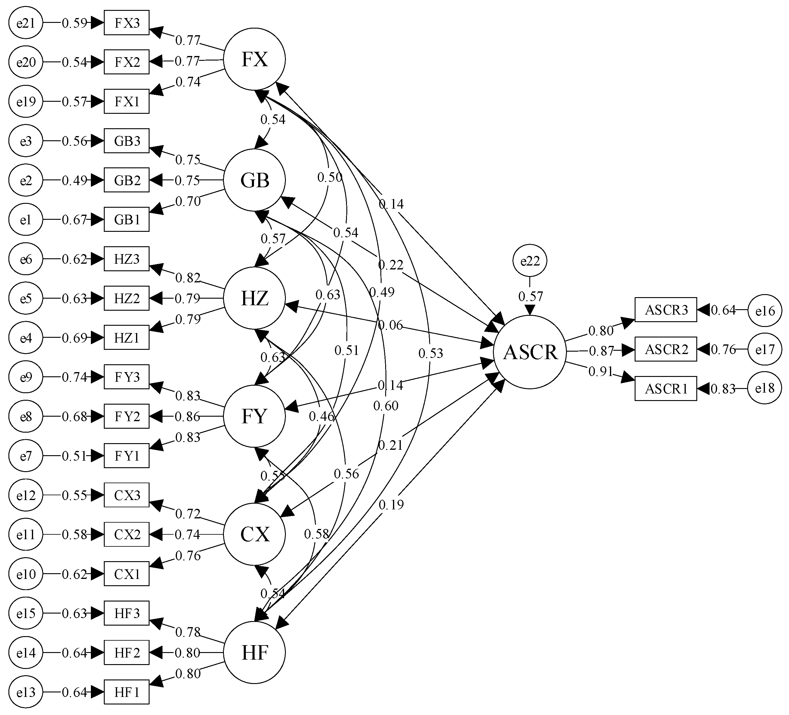
5.1. Method Selection and Model Construction

Based on questionnaire data preprocessing and Structural Equation Modeling (SEM), this study selects five popular machine learning algorithms for comparison with the previously constructed fsQCA-XGBoost model, in order to identify the optimal prediction model. The selected algorithms include Random Forest, Decision Tree, AdaBoost (Adaptive Boosting), ExtraTrees (Extra Randomized Trees), and XGBoost (Extreme Gradient Boosting).

(1) Random Forest Algorithm. The Random Forest algorithm is an ensemble learning method that improves model performance and stability by constructing multiple decision trees and integrating their predictions through voting or averaging. During the construction of the Random Forest, each tree is generated through key steps including row sampling (bootstrap sampling) and column sampling (feature randomness). The algorithm is known for its high accuracy and robustness, demonstrating low sensitivity to noisy data and datasets with redundant features, making it particularly suitable for handling survey-based data. Moreover, the Random Forest algorithm provides the functionality of ranking feature importance and can automatically capture complex interactions between features. The process of selecting splitting features in individual subtrees is illustrated in Figure 3.

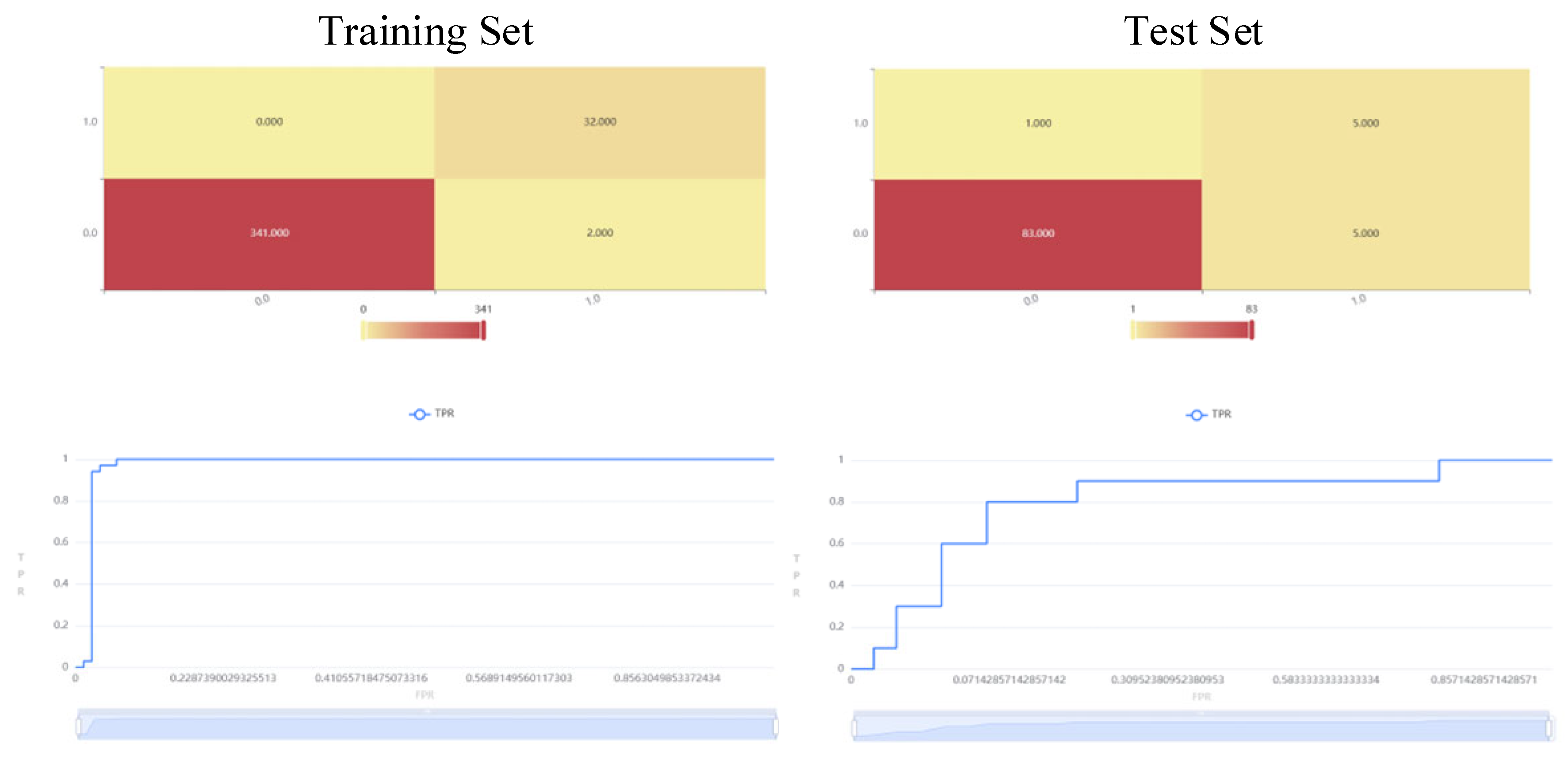
In this study, a Random Forest classification model was first built using the training dataset to obtain the model structure. Subsequently, feature importance scores were calculated based on the trained Random Forest. Finally, the established model was applied to both the training and test datasets to evaluate its classification performance.

The study sets 100 basic decision trees (n_estimators = 100), and adopts the sampling with replacement (Bootstrap) and the feature random subspace strategy (each tree randomly selects “sqrt(total number of features)” features). The optimization ranges of key hyperparameters include the following: the evaluation criterion for node splitting is “gini”, the selection standard for feature split points is “best”, the maximum depth of a single tree “max_depth” is {5, 10, 15}, the minimum number of samples for node splitting “min_samples_split” is {2, 5}, the minimum number of samples for leaf nodes “min_samples_leaf” is {2, 5}, the ratio of the training set to the test set is 8:2, and parameter tuning is performed through five-fold cross-validation to determine the optimal parameter combination, with the goal of maximizing the AUC value. In this study, the bootstrap sampling process is:

$$B_b={\{(x_i^{\left(b\right)},y_i^{\left(b\right)})\}}_{i=1}^n~\mathrm{M}\mathrm{u}\mathrm{l}\mathrm{t}\mathrm{i}\mathrm{n}\mathrm{o}\mathrm{m}\mathrm{i}\mathrm{a}\mathrm{l}(\mathrm{n};{\displaystyle \frac{1}{n}},\dots ,{\displaystyle \frac{1}{n}})$$

(6)

The random subspace projection is:

$$x^{\left(b\right)}=P_{b}x, P_bϵ{\left\{\mathrm{0,1}\right\}}^{m\ast d},{//P_b//}_0=m$$

(7)

where $m=⌊\sqrt{d}⌋=2$, and $P_b$ is the randomly selected matrix.

The decision tree ensemble is constructed as:

$$T_b=arg \underset{T}{\mathit{min}}\sum _{(x,y)ϵB_b}\iota (y,T(P_{b}x)$$

(8)

where $\iota$ is the 0–1 loss function.

The ensemble prediction mechanism is:

$${\widehat{\mathrm{y}}}_{\mathrm{R}\mathrm{F}}\left(\mathrm{x}\right)=\mathrm{sign}(\sum _{b=1}^B{w}_b{T}_b\left(P_{b}x\right))$$

(9)

where $w_b={\displaystyle \frac{1}{B}}$ is the uniform weight.

The configuration feature importance measure is:

$$|\left({\mathrm{C}\mathrm{o}\mathrm{n}\mathrm{f}\mathrm{i}\mathrm{g}}_k\right)={\displaystyle \frac{1}{B}}\sum _{b=1}^B[A\left(T_b,O_b\right)-[A\left(T_b,O_b^{\left(k\right)}\right)]$$

(10)

where $O_b$ is the out-of-bag sample set, $O_b^{\left(k\right)}$ is the out-of-bag sample after feature k is permuted, and A is the accuracy function.

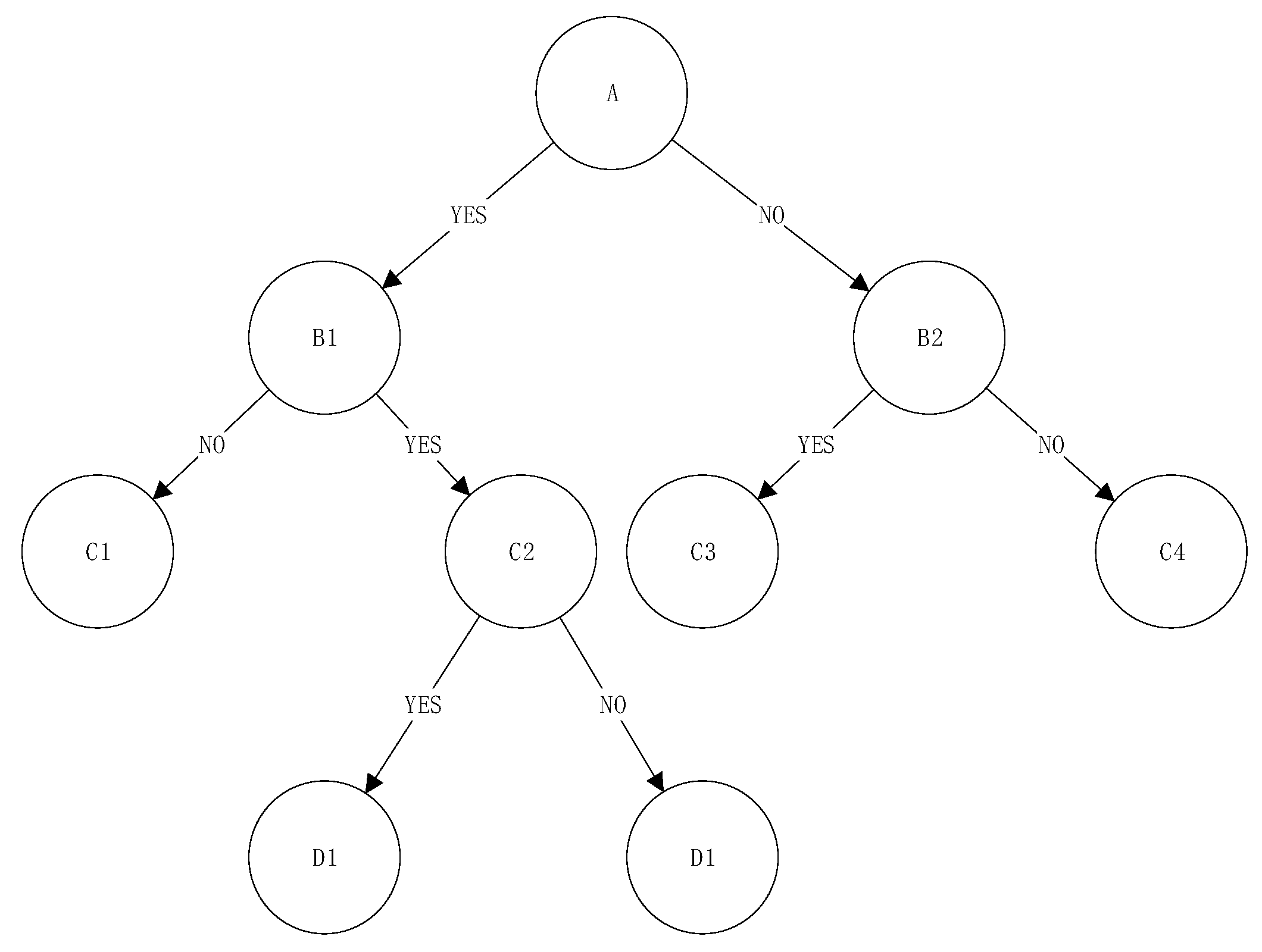
(2) Decision Tree Algorithm. The Decision Tree is a commonly used tree-based algorithm in machine learning for handling both regression and classification tasks. It constructs a tree-like structure through recursive data partitioning, where each node splits the data based on the threshold of a selected feature. This process continues until a predefined stopping condition is met, and the final class label (e.g., high risk/low risk) is output at the leaf nodes. The core mechanism of the Decision Tree involves evaluating potential features for splitting by computing metrics such as information gain (used in the ID3 algorithm) or Gini impurity (used in the CART algorithm). These metrics assess the effectiveness of different features in separating the dataset, thereby enabling the selection of the optimal feature and threshold for node splitting. The Decision Tree algorithm offers strong interpretability due to its transparent decision-making process, and its tree structure can be intuitively visualized. Therefore, it was selected as one of the predictive models in this study. The underlying principle is illustrated in Figure 4.

This paper selects the classic CART algorithm to construct a binary decision tree. During the model construction process, “gini” is selected as the impurity algorithm, the random seed is set to {42}, the feature split point is “best”, the maximum depth of the tree “max_depth” is {3, 5, 7, 10}, the minimum number of samples for leaf nodes “min_samples_leaf” is {3, 5, 10}, and the minimum number of samples for splitting nodes “min_samples_split” is {2, 5, 10}. The ratio of the training set to the test set is 8:2, and parameter optimization is performed through the Grid Search method combined with five-fold cross-validation. The parameter combination with the highest F1-score on the validation set is selected to construct the optimal model. In this study, the feature space is defined as:

$$X={\left\{X_i\right\}}_{i=1}^n, X_i=\left(\begin{array}{c}FX\\ GB\\ \begin{array}{c}DK\\ CX\\ HF\end{array}\end{array}\right)ϵR^5$$

(11)

The standardized transformation is:

$$\Phi \left(\mathrm{x}\right)=D^{-{\displaystyle \frac{1}{2}}}(x-\mu )$$

(12)

where $\mu =E\left[X\right]$ is the feature mean vector, $D=diag\left({\sigma }_1^2,\dots ,{\sigma }_d^2\right)$ is the variance diagonal matrix, and $d=5$.

For the node splitting criterion (CART algorithm), the Gini impurity of node $N$ is defined as:

$$\mathrm{G}\left(\mathrm{N}\right)=1-\sum _{k=0}^1{({\displaystyle \frac{\left|N_k\right|}{\left|N\right|}})}^2$$

(13)

where $N_k=\left\{\right(x,y\left)ϵN\right|y=k\}$.

The optimal split is solved by:

$$\left(f*,t*\right)=\underset{\mathit{fϵF},\mathit{tϵR}}{\mathit{arg\; max}}[G\left(N\right)-\sum _{cϵ\{L,R\}}{\displaystyle \frac{\left|N_c\right|}{\left|N\right|}}G(N_c)]$$

(14)

where $N_L=\left\{\left(x,y\right)|x_f\le t\right\}, N_R=\left\{\right(x,y\left)\right|x_f\ge t\}$.

The resilience level prediction function is:

$$\widehat{y}\left(x\right)=sign(\sum _{j=1}^J{\beta }_j|(xϵL_j))$$

(15)

where $L_j$ is the leaf node region, ${\beta }_j=\log \left({\displaystyle \frac{P_j}{1-P_j}}\right), P_j={\displaystyle \frac{\left|L_{j,1}\right|}{\left|L_j\right|}}$.

(3) AdaBoost (Adaptive Boosting) Algorithm. AdaBoost constructs a strong predictive model by iteratively training weak classifiers—such as decision stumps (decision trees of depth 1). In each iteration, the algorithm adjusts the weights of the training samples: misclassified samples receive higher weights, causing subsequent weak learners to focus more on these difficult cases. Finally, the predictions from all weak classifiers are combined through weighted voting to produce the final output. In this study, which focuses on predicting resilience levels in green agricultural supply chains, high-risk samples are typically in the minority class, only accounting for about 9% of the dataset. The AdaBoost algorithm leverages its weight adjustment mechanism to significantly enhance the detection of high-risk instances, thereby improving the recall performance on imbalanced datasets. This makes it particularly suitable for the present research. The underlying principle is illustrated in Figure 5.

In this study, the AdaBoost algorithm employs decision trees of depth 1 (decision stumps) as weak classifiers, iteratively training through adaptive adjustment of sample weights. Key parameter settings include the following: the number of weak classifiers “n_estimators” set to {50, 100, 200}, the learning rate “learning_rate” set to {0.8, 1.0, 1.2} (controlling the magnitude of weight updates), and the maximum depth of the base classifier “base_estimator__max_depth” fixed at {1} (decision stumps). Grid search combined with five-fold cross-validation is used to optimize parameters, with a focus on recall to enhance the identification of high-risk samples. The feature space is defined as:

$$X={\left\{x_i\right\}}_{i=1}^n, x_iϵR^5$$

(16)

The weak classifier is defined as:

$$h_m\left(x\right)=sign(w_m^T\varphi \left(x\right)+b_m)$$

(17)

where $\varphi \left(x\right)$ is the feature mapping function, and m = 1,2,…,M is the number of iterations.

The iterative optimization process is:

$${ϵ}_m=\sum _{i=1}^n{D}_m\left(i\right)\left|\right(y_i=h_m\left(x_i\right))$$

(18)

$${\alpha }_m={\displaystyle \frac{1}{2}}\mathrm{l}\mathrm{n}({\displaystyle \frac{1-{ϵ}_m}{{ϵ}_m}})$$

(19)

$$D_{m+1}\left(i\right)={\displaystyle \frac{D_m\left(i\right)exp(-{\alpha }_m{y}_i{h}_m\left(x_i\right))}{Z_m}}$$

(20)

where (18) is the weighted error rate, (19) is the classifier weight, (20) is the sample weight update, and $Z_m$ is the normalization numerator.

The ensemble prediction function is:

$$H\left(x\right)=sign(\sum _{m=1}^M{\alpha }_m{h}_m\left(x\right))$$

(21)

The action mechanism of configuration features is:

$${\gamma }_y=\sum _{m:h_m {Config}_k}\left|{\alpha }_m\right|$$

(22)

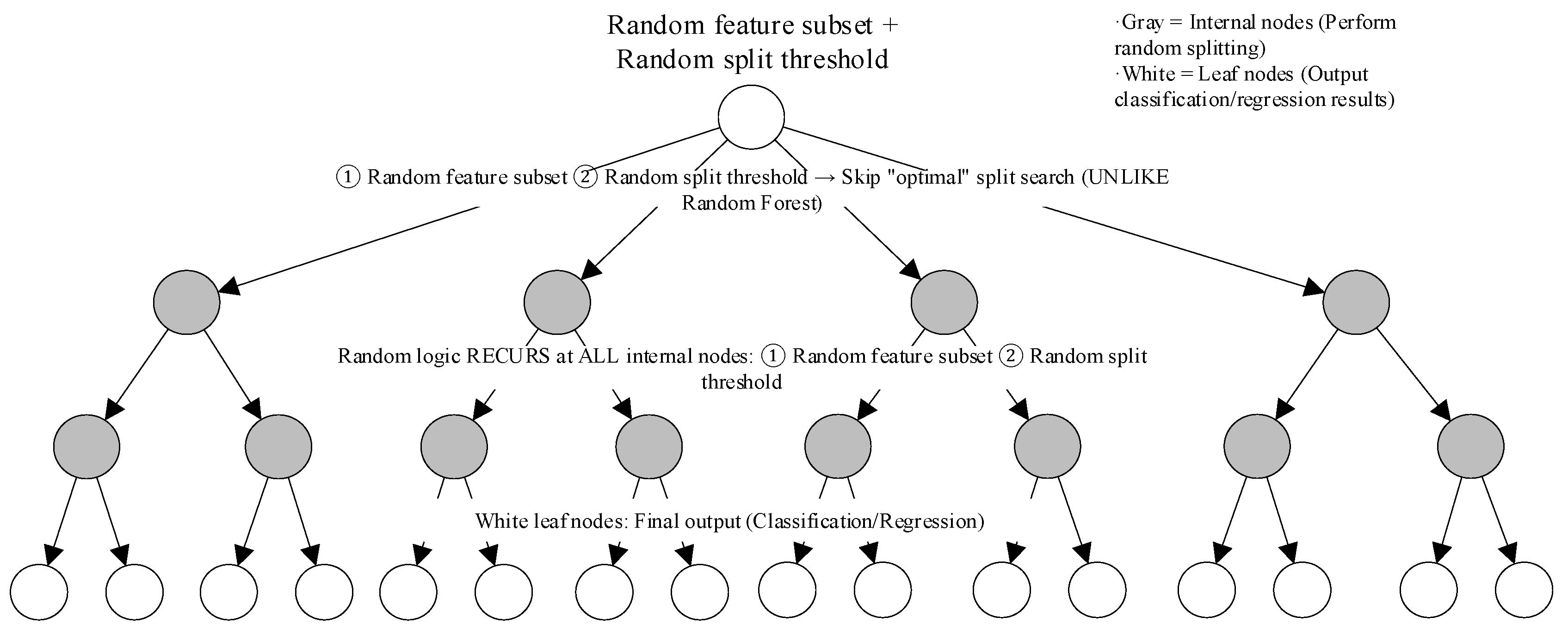
(4) ExtraTrees Algorithm. The ExtraTrees (Extremely Randomized Trees) algorithm is an ensemble learning method based on Random Forests, but it introduces additional randomness during the construction of decision trees. Compared to Random Forests, the key differences lie in its more random splitting and use of the full sample for each tree. During node splitting, ExtraTrees not only randomly selects features but also chooses split thresholds in a random manner. This enhances the model’s generalization ability. Using the full sample for training reduces the variance introduced by bootstrap sampling, thereby further improving the stability of the model. ExtraTrees exhibits high computational efficiency, making it particularly suitable for medium-sized survey datasets (e.g., datasets containing several hundred samples). Additionally, it demonstrates greater robustness when dealing with noisy features (such as redundant items in surveys), effectively reducing the risk of overfitting and ensuring the model’s stability and reliability in practical applications. Therefore, this method was chosen for resilience level prediction in this study. The underlying principle is illustrated in Figure 6.

The model in this paper adopts a gradient boosting framework, using the “binary:logistic” objective function for binary classification tasks. The optimization ranges for key parameters are as follows: learning rate “learning_rate”: {0.01, 0.1, 0.2}; maximum tree depth “max_depth”: {3, 5, 7}; minimum sum of sample weights for leaf nodes “min_child_weight”: {1, 3, 5}; L2 regularization coefficient “reg_lambda”: {0.1, 1, 10}; subsampling ratio “subsample”: {0.8, 1.0}; with the random seed fixed at seed=42. Parameter optimization is performed through 50 rounds of iterative search using Bayesian Optimization, with the F1-score from five-fold cross-validation as the optimization objective. In this study, the extended form of the random forest is:

$$T_b\left(x\right)=Tree(x;{\theta }_b)$$

(23)

where ${\theta }_b$ is the random parameter set.

The extreme random splitting mechanism is:

$$f_b~Uniform(1,d), d=5$$

(24)

$$t_b~Uniform(\underset{i}{\mathit{min}} x_{f_b}^{\left(i\right)},\underset{i}{\mathit{max}} x_{f_b}^{\left(i\right)})$$

(25)

$$\left(f_b*,t_b*\right)=arg\underset{(f,t)\in R_b}{\mathit{max}}\Delta G(f,t)$$

(26)

where (24) is the random feature selection, (25) is the random threshold generation, (26) is the splitting criterion, and $R_b$ is the set of random candidate split points.

The ensemble prediction function is:

$$\widehat{y}=mode{\left\{T_b\right(x\left)\right\}}_{b=1}^B$$

(27)

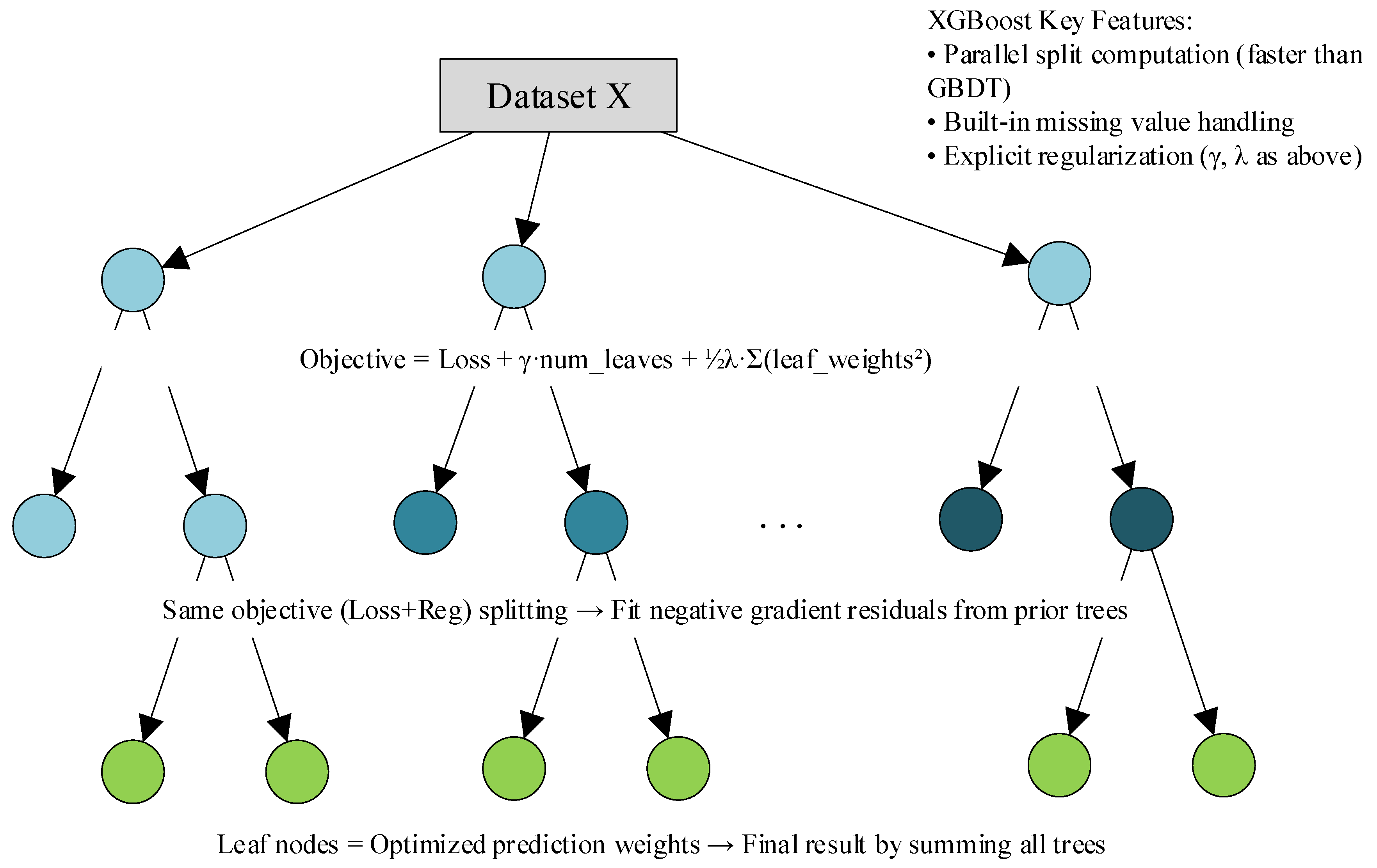
(5) The eXtreme Gradient Boosting (XGBoost) model is an efficient gradient boosting framework. It comprises multiple decision trees, each functioning as a weak classifier, which combine to form a strong classifier. Core advantages of XGBoost include second-order derivative optimization, regularization (L1/L2), and parallel computing. It typically delivers optimal predictive performance in benchmark tests and practical applications across fields. Moreover, by adjusting the “scale_pos_weight” parameter to increase the weight of high-risk samples, XGBoost enhances its performance on imbalanced datasets. The principle behind this is illustrated in Figure 7.

In this study, the XGBoost model employs a gradient boosting framework and uses the “binary:logistic” objective function for binary classification tasks. The optimization ranges for key hyperparameters are as follows: learning rate “learning_rate”: {0.01, 0.1, 0.2}; maximum tree depth “max_depth”: {3, 5, 7}; minimum sum of sample weights for leaf nodes “min_child_weight”: {1, 3, 5}; L2 regularization coefficient “reg_lambda”: {0.1, 1, 10}; and subsampling ratio “subsample”: {0.8, 1.0}. Bayesian Optimization is used for 50 rounds of iterative search, with the F1-score from five-fold cross-validation as the optimization objective. In this research, the core XGBoost model is:

$$\widehat{y_i}=\sum _{t=1}^T{f}_t\left(x_i\right), f_t\in F$$

(28)

Objective Function:

$$L=\sum _{i=1}^n\iota \left(y_i,{\widehat{y}}_i\right)+\sum _{t=1}^T\Omega \left(f_t\right)$$

(29)

where $\iota$ is the logistic loss function: $\iota =-y_{i}log\sigma \left({\widehat{y}}_i\right)-\left(1-y_i\right)\log \left(1-\sigma \left({\widehat{y}}_i\right)\right),\Omega \left(f\right)=\gamma T+{\displaystyle \frac{1}{2}}\lambda {‖w‖}^2$.

Gradient Boosting Framework:

$$L^{\left(t\right)}\approx \sum _{i=1}^n\left[g_i{f}_t\left(x_i\right)+{\displaystyle \frac{1}{2}}{h}_i{f}_t^2\left(x_i\right)\right]+\Omega \left(f_t\right)$$

(30)

$$W_j*=-{\displaystyle \frac{{\sum }_{i\in I_j}{g}_i}{\sum _{i\in I_j}{h}_i+\lambda }}$$

(31)

$$S=-{\displaystyle \frac{1}{2}}\sum _{j=1}^T{\displaystyle \frac{{\left(\sum _{i\in I_j}{g}_i\right)}^2}{\sum _{i\in I_j}{h}_i+\lambda }}+\gamma T$$

(32)

where (30) is the Taylor approximation expansion, (31) is the leaf node weight optimization, and (32) is the structural score. $g_i={\partial }_{\widehat{y}\left(t-1\right)}\iota \left(y_i,{\widehat{y}}^{\left(t-1\right)}\right), h_i={\partial }_{\widehat{y}\left(t-1\right)}^2\iota (y_i,{\widehat{y}}^{\left(t-1\right)})$.

5.2. Results Analysis

To intuitively assess the predictive performance of the models, this study presents a summary of the confusion heatmaps and ROC curves for both the training and test sets across all algorithms, as shown in Figure 8.

The results indicate that all five machine learning algorithms identified resource recycling agility (FY) as a core risk factor, with feature importance ranging from 30.40% to 59.25% (

Table 7. AUC Results and Feature Importance of FY across Machine Learning Algorithms.

Algorithm	Test Set Recall	Test Set F1-Score	Test Set AUC	Feature Importance of Agility (FY)
Random Forest	0.90425	0.87568	0.54967	49.88%
Decision Tree	0.89361	0.89830	0.75359	59.25%
AdaBoost	0.85106	0.84046	0.84732	33.09%
ExtraTrees	0.86170	0.85201	0.85542	30.40%
XGBoost	0.92553	0.91600	0.76190	47.53%

). This confirms the fundamental impact of resource recycling resilience on supply chain disruptions. However, this single-dimensional strong dependency exposes a fundamental limitation of traditional machine learning in resilience level prediction. (1) Decision Tree: Due to excessive focus on FY, it suffers from rigid decision boundaries (test set AUC = 0.754), failing to respond to complex risk patterns formed by multiple interacting factors. (2) Ensemble Models (RF/XGBoost): Although these models attempt to integrate multiple features, they suffer from noise interference (RF AUC = 0.550, XGBoost AUC = 0.762) and dilution by weak features (e.g., ExtraTrees with a 6.69% contribution from low-importance features). (3) AdaBoost: Despite achieving the highest AUC (0.847), its iterative sample weight adjustment mechanism amplifies the influence of noisy samples, leading to fluctuations in high-risk sample recall rates (F1-score < 0.80). None of the algorithms achieved an AUC exceeding the effective threshold (0.90) on the test set. The core issues include: (1) Distorted Risk Signal Extraction: Over-reliance on a single feature (FY) neglects the synergistic effects of multiple factors, leading the model into a “missing the forest for the trees” decision trap. (2) Lack of Noise Filtering Mechanism: Weakly correlated features (e.g., education level) introduce spurious correlations during ensemble processes, diluting true risk signals. (3) Insufficient Dynamic Adaptability: Existing algorithms fail to capture asymmetric combinations of risk factors (e.g., “high FY + low CX” may trigger risks, while “low FY + high CX” has no effect). These findings highlight the inadequacy of traditional machine learning in modeling the multifactorial and nonlinear coupling characteristics of supply chain risks. There is an urgent need to introduce analytical frameworks capable of parsing conditional configurations to address these limitations. Detailed results are presented in Table 7.

It is evident that, compared to conventional machine learning predictive models, the fsQCA-XGBoost resilience prediction model has achieved a breakthrough in performance: (1) From Single-Point Dependency to Configurational Synergy: Compared to the best-performing XGBoost among the five classic predictive models, which rely on a single operational feature and overlook the “policy–technology–market” synergy mechanism identified by fsQCA, the new model incorporates configurational features (con1–con4) to fully capture the theoretical framework and quantify multifactorial coupling effects. Additionally, the new model achieves noise filtering by eliminating irrelevant variables such as “education level” (originally comprising 6% of the feature space), thereby increasing the purity of the feature space by 100%. (2) Significant Enhancement in High-Risk Sample Recognition: Compared to the original model, the new model shows an improvement of 66% in recall rate and over 150% in positive sample identification. The risk of false negatives has been reduced by 50%. The new model’s ability to capture high-risk samples (positive class) has increased threefold, significantly improving upon the “missing the forest for the trees” flaw of the original model. (3) Qualitative Improvement in Generalization Ability: From Overfitting to Robust Prediction: The AUC improvement of the fsQCA-XGBoost resilience prediction model exceeds 19%, with the gap between training and test set performance reduced by 61.3%. This addresses the generalization error where the original model had a high AUC on the training set but a low AUC on the test set, achieving a doubling of early risk detection efficiency. (4) Optimized Error Mechanism: From Random Misclassification to Explainable Bias: In the original model, false positives and false negatives were random and untraceable. However, in the improved model, errors can be traced back to the fsQCA configurational theory (e.g., false-negative data are boundary samples of Configuration 3). This provides explainable improvement anchors for dynamic risk warning (see Table 5, Table 6 and Table 7, Figure 2 and Figure 8).

6. Conclusions

6.1. Research Conclusions

The stability of green supply chain systems plays a critical role in achieving the “dual carbon” goals (carbon peaking and carbon neutrality). This study first synthesizes relevant literature to identify influencing factors of resilience in green supply chains. Subsequently, a Structural Equation Model (SEM) is employed to uncover key determinants, ultimately identifying five influencing factors across three dimensions. Building on this foundation, the study further constructs predictive models for supply chain disruption risks using multiple machine learning algorithms. Finally, based on fsQCA configurational analysis, an accurate prediction model—the fsQCA-XGBoost model—was developed. Research findings indicate that supply chain resilience is fundamentally a systemic capability driven by a policy–technology–market triple helix synergy, with the institutional compensation pathway (Configuration 3) emerging as the key mechanism to resolve the “agility paradox”, contributing 49.64% of the predictive weight. Compared to traditional machine learning models that excessively rely on single operational features, the new model has made breakthroughs in two aspects through reconstructing the configuration characteristics:

1. Theoretical Validation of Configurational Synergy Mechanisms. This study reveals the multiple pathway mechanisms underlying the formation of green logistics resilience through Structural Equation Modeling (SEM) and fuzzy-set Qualitative Comparative Analysis (fsQCA). It finds that high-resilience green logistics systems do not rely on the linear superposition of a single condition, but rather achieve substitution through differentiated configurational pathways of “policy tools–technological innovation–market response,” verifying these four configurational pathways. (1) Boundary conditions for institutional compensation of technological shortcomings. In the fsQCA configurational analysis, the compensation breakthrough pathway highlights the importance of policies and collaborative innovation, suggesting that agility may indirectly take effect when they are combined [73]. For example, small and medium-sized enterprises in the Beijing–Tianjin–Hebei region can enhance resilience by shortening recycling cycles through government-shared cold storage and blockchain traceability technology, despite lacking hardware redundancy. This may indicate that resource circulation agility needs to be embedded in institutional frameworks and technological networks to be converted into resilience gains, which not only echoes the dynamic capability theory but also confirms the “compensatory boundary of policy intervention in market failure” in institutional theory [67]. (2) Nonlinear synergy of core variables. The fsQCA configurations identify four resilience pathways: collaborative-driven, dual-adaptive, compensation breakthrough, and dual-wheel-driven. Their commonality lies in the central role of internal monitoring and feedback, as well as collaborative innovation, which also verifies the core proposition of “multiple conjunctural causality” in complex adaptive systems theory [74,75]. This indicates that green logistics resilience is the result of the triple helix coupling of policy, technology, and market. Policy flexibility (e.g., dynamic allocation of carbon quotas) [76] provides a legitimate framework for enterprises to resume low-carbon operations, while market responses (e.g., switching between multimodal transport) verify the effectiveness of policy tools, forming a “monitoring–adjustment–verification” loop [77]. (3) Threshold constraints and complementarity of innovation capability. Innovation capability serves as a core condition in the collaborative-driven and dual-wheel-driven pathways, indicating that its role in green resilience significantly depends on critical conditions, and its effectiveness can only be released on the premise of infrastructure redundancy or policy guidance. This may be explained through the following mechanisms: ① Technology-facility matching effect. Green technological innovations (e.g., hydrogen energy cold chain, blockchain-based carbon tracing) need to be matched with specific hardware conditions to be implemented [34]. For instance, when enterprises in the Yangtze River Delta initially deployed hydrogen-powered vehicles, the related technologies were still immature and failed to significantly reduce carbon intensity. However, governments and enterprises heavily invested in photovoltaic facilities, supporting hydrogen-powered vehicles’ nighttime energy replenishment through redundant electricity, thereby achieving carbon reduction. This suggests that innovation capability must cross the critical point of “technological feasibility–operational economy,” and that redundancy (e.g., energy overcapacity) reduces the cost of technological trial-and-error by providing buffer resources and stabilizing the physical environment, thereby amplifying the marginal benefits of technological innovation. ② Policy-innovation risk hedging effect. When technological maturity is insufficient, enterprises’ innovation investments face high risks. Governments (i.e., issuers of institutions) can significantly reduce enterprises’ innovation costs through means such as low-carbon subsidies, as seen in the “green consumption vouchers” and “R&D subsidies” in the Chengdu–Chongqing region. This indicates that policy tools can drive technologies across the market acceptance threshold by reducing the marginal cost of innovation.

2. Paradigm-Level Advancement in Predictive Performance. Compared with the original XGBoost model, the hybrid model achieves a 19% increase in AUC (Area Under the Curve) on the test set and a 50% reduction in the omission rate of high-risk samples, marking a qualitative shift in the prediction paradigm from “single-point vulnerability scanning” to “multi-pathway synergistic diagnosis”. Specifically, first, there is a breakthrough in generalization ability: it not only effectively addresses the overfitting issue of the original model but also locates the sources of errors through configurational vulnerability points, thereby realizing the traceability of causal mechanisms. Second, it optimizes early risk detection: the true positive rate is significantly improved, and the combination of low false-positive rates and high true-positive rates creates a critical time window for dynamic intervention. Third, it provides a theoretically traceable basis for error mechanisms through configurational vulnerability points, converts fsQCA configuration membership degrees into input features for machine learning, realizes the interpretability optimization of the model, and thus overcomes the flaw of “disconnection between statistical models and theory”.

6.2. Practical Implications

1. Construct a “monitoring–reconstruction–compensation” resilience governance system on the government side. For technology-leading regions (e.g., the Yangtze River Delta), mandatory certification for hydrogen-powered cold chain equipment can be implemented, accompanied by infrastructure standards with a photovoltaic redundancy rate of ≥30%. For export-oriented regions (e.g., the Guangdong–Hong Kong–Macau Greater Bay Area), a cross-border carbon accounting whitelist can be established, and a flexible collection and management mechanism for turnover tax can be implemented for multimodal transport switching. For capital-constrained regions (e.g., Beijing–Tianjin–Hebei), accelerated depreciation plus additional deductions for shared cold storage can be provided to reduce the marginal cost of asset-light transformation. Secondly, based on the research model, a “Green Logistics Resilience Index” can be developed, generating quarterly regional risk heatmaps as a quantitative allocation basis for special transfer payments for carbon emission reduction. Finally, fund research institutions to develop a policy–technology coupling decision console (e.g., correlation algorithms between carbon price fluctuations and photovoltaic output) to improve the self-sufficiency rate of cold chain energy.

2. For enterprises, strategic anchors of configurational pathways should be embedded in a stratified manner. Leading enterprises should be encouraged to lead hydrogen cold chain technology standard alliances (e.g., SF-led cold-start time compression laboratories) to compress equipment cold-start time to ≤2 h (a 50% improvement compared to the current situation). Small and medium-sized enterprises should be encouraged to access the government’s intelligent scheduling system for shared facilities (e.g., the Beijing–Tianjin–Hebei algorithm platform) to improve facility utilization (avoiding heavy asset investment risks). Industry associations should jointly promote the formulation of Cross-Regional Green Logistics Resilience Certification and Mutual Recognition Standards to reduce duplicate compliance costs between the Yangtze River Delta and the Guangdong–Hong Kong–Macau Greater Bay Area. Financial institutions should attempt to innovate “carbon price threshold-triggered insurance” (automatic claims settlement when carbon price fluctuations exceed critical values) and incorporate configurational adaptability into ESG rating weighting factors.

3. At the social level, efforts should be made to promote the construction of a collaborative network for low-carbon behaviors. For producers, lightweight low-carbon technology packages (small photovoltaic cold storage modules) and pilot projects for Marginal Abatement Credit (MAC) trading should be promoted. For consumers, carbon label visualization projects (A–E grade carbon emission labels for fresh produce packaging) and grid-based coverage of community low-carbon education should be implemented.

6.3. Theoretical Contributions

This study achieves three breakthroughs at the theoretical level:

1. Deconstructive breakthrough in configurational causal mechanisms. Breaking away from the reliance of traditional linear models on single factors, this study reveals that the resilience of agricultural product green supply chains is a product of complex systems shaped by the “policy–technology–market” triple helix synergy. Among them, Configuration 3 verifies “the compensatory mechanism of institutional innovation for technological shortcomings”; Configuration 2 refines the boundary conditions of policy intervention in institutional theory. This finding subverts the linear assumption of a single technology or policy as the driver in traditional research, clarifying the core role of multi-factor asymmetric interactions (e.g., “high agility + low innovation” may trigger risks, while “low agility + high innovation” has no significant impact).

2. Paradigmatic leap in predictive methodology. The innovative construction of the fsQCA-XGBoost hybrid framework realizes a breakthrough from “single-algorithm prediction” to “causal-prediction closed loop”. This framework not only retains fsQCA’s causal explanatory power for configurational pathways but also leverages XGBoost’s capability in modeling high-order interactions, leading to a significant increase in the test set AUC and a 66% optimization in the recall rate of high-risk samples. It provides a hybrid methodological paradigm of “causal explanation + accurate prediction” for resilience prediction in complex systems.

3. Reconstruction of decision support tools. Translating theoretical findings into operable decision tools, through regional resilience heatmaps constructed based on configurational membership degrees and differentiated governance anchors, this study achieves a paradigm shift from “post-event remediation” to “critical point early warning”. This instrumentalization process verifies the practical value of complex adaptive systems theory in supply chain management, transforming the collaborative goals of “carbon reduction–supply stability–efficiency improvement” from abstract theories into quantifiable and intervenable specific indicators, thus providing methodological support for the implementation of relevant theories.

6.4. Research Limitations and Future Directions

Although this study confirms the core role of multiple concurrent causal relationships in green supply chain resilience, there are still some limitations. First, due to reliance on cross-sectional survey data from 768 respondents, this study lacks dynamic analytical capabilities and cannot capture the long-term impacts of policy iterations (e.g., tightening of carbon quotas) and technology diffusion (e.g., declining hydrogen costs) on configurational paths. Unlike longitudinal data, which can verify the dynamic evolution of resilience paths over time, the cross-sectional design limits our ability to track how configurational effects shift as the system changes. Second, there are generalizability constraints, both at the industry level and the institutional level. The sample is mainly derived from agricultural product supply chains, and the relevant conclusions need to be verified before being extended to high-value-added industries such as electronics and pharmaceuticals. Moreover, since the current analysis is based on the specific policy and market environment in the studied agricultural product field, the transferability of research conclusions to supply chains operating under other institutional or regulatory systems may be limited. Third, there are cross-border applicability barriers: this study does not cover fragmented carbon accounting standards along the “Belt and Road Initiative” (e.g., differences between ASEAN’s CLMVS and the EU’s CBAM), nor does it develop cross-border configurational adaptation algorithms. Finally, the study relies on self-reported data from questionnaires, which may introduce measurement bias—respondents’ subjective perceptions (e.g., perceptions of policy effectiveness or technology maturity) may deviate from objective reality, which could further affect the accuracy of the constructed models.

Based on the above, this paper suggests future research directions as follows. First, future research could focus on the dynamic evolution mechanism of configurations. Introduce time-series fsQCA to track the interactive effects of policy instruments (such as subsidy reduction gradients) and technological maturity (electrolyzer cost curves) to identify thresholds for shifts in the “compensation → breakthrough” type of resilience. Second, develop early-warning systems with multi-source data fusion. Integrate high-granularity IoT data (0.1 Hz sampling of cold chain temperature and humidity + real-time energy consumption of transport vehicles) with supply chain survey data to construct a dual-dimensional physical–social risk radar chart. Third, optimize the robustness of cross-border scenarios. For example, develop cross-institutional configuration-transfer algorithms and establish a resilience-adaptation index for diverse regulatory environments. Finally, expand industry-comparison research. For instance, focus on electronic supply chains (in chip-shortage scenarios) and pharmaceutical supply chains (with vaccine cold chain interruptions) to verify the universality of the “technology–institution” coupling mechanism and extract industry-specific resilience paths.