A Hybrid CNN–BiLSTM Framework Optimized with Bayesian Search for Robust Android Malware Detection

Abstract

With the rapid proliferation of Android smartphones, mobile malware threats have escalated significantly, underscoring the need for more accurate and adaptive detection solutions. This work proposes an innovative deep learning hybrid model that combines Convolutional Neural Networks (CNNs) with Bidirectional Long Short-Term Memory (BiLSTM) networks for learning both local features and sequential behavior in Android applications. To improve the relevance and clarity of the input data, Mutual Information is applied for feature selection, while Bayesian Optimization is adopted to efficiently optimize the model’s parameters. The designed system is tested on standard Android malware datasets and achieves an impressive detection accuracy of 99.3%, clearly outperforming classical approaches such as Support Vector Machines (SVMs), Random Forest, CNN, and Naive Bayes. Moreover, it delivers strong outcomes across critical evaluation metrics like F1-score and ROC-AUC. These findings confirm the framework’s high efficiency, adaptability, and practical applicability, making it a compelling solution for Android malware detection in today’s evolving threat landscape.

1. Introduction

The proliferation of Android devices—driven by their affordability, open-source nature, and widespread market presence—has made the platform a prime target for mobile malware. The availability of alternative app distribution platforms and the fundamental openness of the Android ecosystem further shape an environment favorable to the spread of malicious applications. Reports indicate a sharp rise in Android-targeted malware, with earlier estimates suggesting that a new malicious app emerged every seven seconds as early as 2018 [1,2,3]. According to AV-TEST, there were approximately 6.06 billion recorded malware attacks worldwide in 2023, marking a 10% rise compared to the previous year. As of 2024, the situation continues to deteriorate, with daily detections exceeding 450,000 new malware variants and potentially harmful applications (PUAs) by cybersecurity experts. This ongoing surge in threats reflects the increasing sophistication of Android malware and highlights the urgent need for more intelligent and resilient detection strategies [4].

Android malware appears in multiple forms, including trojans, ransomware, spyware, adware, and riskware, with each variant engineered to take advantage of specific flaws in the operating system or in user behavior [5,6,7]. According to Kaspersky, adware represented 46% of all mobile threats in Q1 2024, while RiskTool-type apps (categorized as riskware) accounted for 21.27% of detections [8,9]. The continued dominance of these threats underscores the persistent challenges in mobile security and the adaptive nature of malware authors. This diversity in malware functionality necessitates detection systems capable of analyzing both behavioral and structural patterns.

To mitigate these growing threats, researchers have developed a variety of detection strategies, including techniques such as static and dynamic program inspection, along with conventional machine learning and modern deep learning methodologies [10,11,12]. Although traditional detection systems have proven useful, they often struggle to counter advanced evasion strategies employed by modern and highly sophisticated malware variants [11,13]. In contrast, recent research highlights the potential of deep learning models, which are particularly effective at identifying intricate behavioral patterns and irregularities that static and rule-based systems frequently miss [10,14,15]. Among these, hybrid deep learning architectures have demonstrated particular promise, as they integrate mechanisms to extract both localized and sequential characteristics of application behavior, resulting in notable gains in detection accuracy and model resilience.

In light of this, the current research proposes a hybrid framework for Android malware detection that combines Convolutional Neural Networks (CNNs) with Bidirectional Long Short-Term Memory (BiLSTM) layers. To optimize the model, Mutual Information (MI) was chosen for feature selection due to its ability to capture non-linear dependencies between features and the target variable, its model-independence, and its efficiency in large feature spaces. Unlike wrapper-based methods such as Recursive Feature Elimination [10] or filter-based methods like chi-square, MI avoids classifier-specific biases and reduces computational overhead—critical in high-dimensional Android malware datasets [11]. Bayesian Optimization is then employed to systematically adjust key hyperparameters and maximize model efficiency. This architecture was selected due to its synergistic advantages: CNNs are well-suited for extracting localized behavioral signatures from app activity, and BiLSTMs effectively capture temporal patterns in both forward and backward sequences—essential for identifying complex malware behavior. When compared with earlier configurations, including those using LSTM–GRU chains or tuning methods based on the Earthworm Optimization Algorithm, this model exhibits superior accuracy, achieving a detection rate of 99.3%. The system has been rigorously validated using publicly available Android malware datasets and shows strong adaptability across a wide range of attack types and evaluation benchmarks.

The remainder of this paper is structured as follows: Section 2 provides a review of the related literature. Section 3 outlines the methodology employed in this study. Section 4 describes the experimental setup and presents the simulation results. Section 5 concludes the study and suggests potential avenues for future work.

2. Related Work

Recent advances in Android malware detection have seen a shift toward deep learning-based models, particularly those employing CNNs for automated feature extraction. Yu et al. [16] introduced a CNN-based approach that treated malware binaries as grayscale images, enabling classification through image recognition techniques. While effective in capturing visual patterns, the model’s high computational complexity poses challenges in real-time or resource-constrained environments. Moreover, its susceptibility to previously unseen obfuscation techniques limits its generalizability to evolving malware families.

To improve classification accuracy, researchers have increasingly explored feature selection techniques as a preprocessing step for traditional and deep learning models. Alamro et al. [17] proposed a multi-level feature selection framework that identified Optimal Static Feature Sets (OSFSs) and Most Important Features (MIFs) using a combination of machine learning algorithms. Their model achieved 96.2% accuracy using Random Forest classifiers. However, the reliance on static code attributes makes it less effective in capturing dynamic behavioral traits, and its performance may degrade across diverse malware datasets due to feature set dependency.

Other studies have emphasized cloud-native infrastructure and alternative approaches to feature engineering. Fevid et al. [18] proposed a cloud-integrated malware detection system, CloudIntellMal, utilizing Amazon Web Services (AWSs) to enable scalable data handling and computation. The framework applies a “Bag of n-grams” technique for feature extraction and shows strong results on the AMD dataset. While the approach is innovative, it lacks deep sequential modeling and spatial feature analysis, which limits its capacity to identify intricate behavioral patterns present in advanced Android malware.

Building on the strengths of both static and dynamic analysis techniques, Smmarwar et al. [19] proposed a deep learning-based malware detection system that interprets Portable Executable (PE) files as RGB images, allowing Convolutional Neural Networks (CNNs) to extract spatial features. Their model reported a detection accuracy of 99.06% on the Malimg dataset, surpassing several contemporary methods. Despite its promising results, the approach incurs high computational overhead and depends heavily on extensive data augmentation, which poses challenges for scalability and real-time deployment, especially in mobile contexts. Additionally, since the model is trained and tested primarily on Windows-based PE files, its relevance to Android malware detection remains limited.

In contrast, Shaukat [20] proposed a risk assessment framework based on machine learning to analyze Android applications. The method relies on evaluating app permissions to identify malicious intent, demonstrating strong performance across datasets such as M0Droid, Androzoo, and Drebin. Although effective in detecting privacy breaches, the model’s reliance on static permission attributes limits its resilience, especially against obfuscated or adversarially crafted applications. This limitation underscores the necessity for more resilient, behavior-driven detection systems that can capture both temporal dynamics and contextual patterns within application behavior.

Beyond individual deep learning architectures, ensemble and hybrid approaches have gained traction in malware detection. Dai et al. [21] proposed a parallel ensemble framework that combines several base classifiers with a neural meta-layer to boost detection accuracy. Their system incorporates Backpropagation and Particle Swarm Optimization (PSO) for fine-tuning and reported strong results across multiple datasets. Similarly, Shaukat [20] presented DMMal, a few-shot learning approach that improves semantic representation using multi-channel malware imagery and sharpness-aware optimization. Despite their effectiveness, these strategies often rely on intricate ensemble designs or elaborate data augmentation processes. In contrast, the CNN–BiLSTM architecture proposed in this study offers a more concise yet effective alternative, integrating spatial and temporal modeling with Mutual Information-based feature selection and Bayesian hyperparameter optimization to achieve robust Android malware detection.

Beyond neural architectures and ensemble-based strategies, behavioral similarity-based methods have also emerged as promising alternatives for Android malware detection. Zhu et al. [22] introduced Andro-AutoPsy, a detection system that leverages similarity analysis grounded in both behavioral patterns and author-linked metadata to group and identify malicious applications. The framework proved effective in uncovering zero-day threats by constructing composite behavioral profiles. Nevertheless, its dependence on predefined similarity criteria may hinder its capacity to differentiate between variants that are behaviorally similar yet functionally distinct, particularly in dynamic threat environments where malware evolves rapidly beyond established patterns. Likewise, Mohaisen et al. [23] developed AMAL, a behavior-based automated malware analysis framework that groups malware samples by behavioral similarity, demonstrating high-fidelity classification. However, these methods often depend on predefined similarity metrics, limiting their adaptability against functionally distinct but behaviorally similar variants.

Alasmary et al. [24] proposed a graph-based system for detecting emerging IoT malware by modeling structural dependencies within control flow graphs. Abusnaina et al. [25] extended this work with DL-FHMC, a fine-grained hierarchical deep learning framework for robust malware classification. Despite their effectiveness, such graph-based solutions often entail substantial computational costs and deployment complexity, making them less suitable for lightweight, on-device malware detection. Alasmary et al. [26] introduced Soteria, a defense mechanism targeting adversarial examples in graph-based malware classifiers.

In recent years, Large Language Models (LLMs) have also emerged as a promising paradigm for program analysis and malware detection tasks. Wang et al. [27] conducted a comprehensive survey of LLM-assisted program analysis, highlighting how models like GPT can analyze code semantics and vulnerabilities with high fidelity. Similarly, Gu et al. [28] proposed an iterative hybrid program analysis approach leveraging LLMs for automated test generation. These advancements demonstrate the potential of LLMs to enhance malware detection by understanding complex software behaviors and adapting to obfuscated code. While still an emerging field, integrating LLM-based techniques with existing deep learning frameworks could open new avenues for robust and adaptive Android malware detection systems.

Ali et al. [29] introduced a layered hybrid Bayesian belief network aimed at identifying Advanced Persistent Threats (APTs). Their approach integrates static code analysis, runtime behavior monitoring, and event-based evaluation within a hierarchical Bayesian structure, achieving a detection rate of 92.62% alongside an exceptionally low false-positive ratio. While effective in modeling sophisticated attack vectors, the method’s high architectural complexity and significant computational requirements make it less suitable for deployment in real-time or mobile contexts. Moreover, the framework is primarily tailored for enterprise-level security scenarios, limiting its adaptability to the broader and more dynamic landscape of Android malware targeting consumer devices. Similarly, Shen et al. [30] introduced a complex-flow-based model for Android malware detection, showing high performance but with substantial runtime costs.

Feature selection remains a pivotal factor in enhancing both the speed and accuracy of malware detection models. In a related effort, Ibrahim et al. [31] investigated the use of genetic algorithms to identify the most relevant features for Android malware detection across nine machine learning classifiers. Their approach yielded notable gains in both classification performance and computational efficiency when compared to traditional information gain techniques. Nonetheless, the study primarily focused on evolutionary selection methods and did not thoroughly assess more contemporary alternatives like Mutual Information or Recursive Feature Elimination. In contrast, this research adopts Mutual Information as a lightweight yet powerful technique to refine feature relevance, contributing to improved learning efficiency when integrated into a CNN–BiLSTM-based deep learning framework.

In the area of optimization-integrated malware detection, Maray et al. [32] developed a system named AAMD-OELAC, which integrates multiple classifiers, namely Least Squares Support Vector Machine (LS-SVM), Kernel Extreme Learning Machine (KELM), and Random Vector Functional Link Network (RRVFLN), into an ensemble framework. The ensemble’s parameters are refined using the Hunter–Prey Optimization (HPO) algorithm to enhance classification accuracy. Although the approach delivers strong detection performance, its dependence on multiple models and a computationally intensive optimization strategy limits its practicality for real-time mobile environments. In comparison, this study utilizes Bayesian Optimization, a more streamlined and scalable method for hyperparameter tuning, embedded within a single, cohesive deep learning framework.

Moreover, dynamic analysis methods have been introduced to more effectively capture malicious behaviors during an app’s execution. Ji et al. [33] introduced HeteroNet, a deep learning-based solution that leverages diverse runtime characteristics by combining API call sequences, resource utilization graphs, and function call graphs. Achieving a precision of 98.40%, the model outperforms conventional baselines. However, its reliance on multi-modal data inputs and complex architectural components results in high computational overhead, which limits its suitability for mobile or resource-constrained environments. In contrast, the proposed CNN–BiLSTM framework achieves a more efficient balance between behavioral insight and system performance by integrating effective feature selection with Bayesian-optimized training—delivering high accuracy without compromising scalability.

Shu et al. [34] tackled the issue of limited labeled data in Android malware detection by utilizing a Siamese neural network within a one-shot learning paradigm. Their approach achieved 98.9% accuracy on the Drebin dataset and showed promise in identifying various malware families. Nevertheless, one-shot learning methods are generally most effective when intra-class variation is minimal, which can hinder their performance in recognizing novel or highly diverse malware. Furthermore, the model’s heavy reliance on the Drebin dataset restricts its applicability to wider malware ecosystems, emphasizing the importance of training on more heterogeneous datasets for improved generalization.

Pinhero [35] proposed a deep learning approach for malware image classification that fine-tunes a pre-trained VGG19 model to address class imbalance. Their method achieved 99.72% accuracy on the Malimg dataset by transforming malware binaries into visual representations. While promising, the reliance on transfer learning from pre-trained networks may reduce adaptability to unseen or fundamentally different malware patterns. Moreover, the method’s sensitivity to dataset imbalance suggests limitations when applied to real-world malware data, where class distributions are often highly skewed.

Sinha et al. [36] investigated image-based malware classification through IMCEC, an ensemble of CNN models tailored to detect both packed and unpacked Android threats. Their approach delivered impressive performance, “achieving accuracy rates exceeding 99% for unpacked samples and around 98% for packed ones,” by utilizing diverse CNN configurations to extract comprehensive feature patterns. However, the ensemble nature of the model resulted in substantial computational demands, limiting its suitability for lightweight or real-time environments. In comparison, the CNN–BiLSTM framework introduced in this study achieves similarly high detection accuracy with a more streamlined architecture that integrates spatial and temporal learning. Moreover, the application of Mutual Information for selecting relevant features and the use of Bayesian Optimization for tuning hyperparameters contribute to the model’s efficiency and adaptability across varied Android malware datasets.

Surendran et al. [37] proposed an intelligent recognition system for detecting Android malware by integrating the Equilibrium Optimizer (EO) with a Long Short-Term Memory (LSTM) network enhanced by channel attention mechanisms. Their IPR-EODL architecture achieves notable classification accuracy by leveraging EO for fine-tuning deep learning model parameters. Nonetheless, the high computational overhead associated with CA-LSTM layers, coupled with EO’s reliance on carefully initialized parameters, raises scalability concerns—particularly in time-sensitive or resource-constrained environments. Moreover, the framework’s adaptability to rapidly evolving malware families and previously unseen datasets has not been thoroughly validated.

Isohanni [38] introduced a deep learning approach for Android malware family classification using a ResNet-50 architecture, where malware binaries are transformed into grayscale byteplot images. By fine-tuning the final layer of a ResNet-50 model originally trained on ImageNet, they achieved a detection accuracy of 98.62%. Despite its strong performance, the reliance on a large pre-trained convolutional network reduces adaptability to emerging malware variants and introduces substantial computational demands, making the approach less suitable for resource-constrained or mobile environments.

Das et al. [39] developed the RHSODL-AMD model, which combines Rock Hyrax Swarm Optimization (RHSO) with a deep learning-based architecture for Android malware detection. Feature selection is performed using an RHSO-based subset selection method on API calls and permissions, followed by classification using an attention-based recurrent autoencoder (ARAE) optimized with Adamax. The model achieved 99.05% accuracy on the Andro-AutoPsy dataset. However, its reliance on complex optimization techniques and customized feature selection strategies may hinder adaptability across varied datasets and increase implementation complexity, particularly in real-time scenarios.

In contrast, the proposed framework in this study leverages a streamlined yet powerful hybrid CNN–BiLSTM architecture that balances detection performance with computational efficiency. By employing Mutual Information for lightweight and effective feature selection and Bayesian Optimization for adaptive hyperparameter tuning, the model achieves high accuracy while ensuring scalability, generalizability, and practical applicability in dynamic Android malware detection environments. The comparative summary in Table 1 clearly demonstrates how our approach outperforms prior studies in terms of detection accuracy, dataset diversity, and reduced computational overhead.

Table 1. Summary of Android malware detection approaches.

Study	Approach	Dataset	Evaluation Metric(s)	Accuracy (%)	Our Approach
Yu et al. [14]	CNN on Grayscale Malware Images	Malimg	Accuracy	97.5	CNN–BiLSTM, Mutual Info + BO
Alamro et al. [15]	OSFS + Random Forest	Drebin	Accuracy, F1-score	96.2	Achieves higher accuracy (99.3%)
Fevid et al. [16]	CloudIntellMal with n-grams	AMD	Precision, Recall	95.8	Lightweight, faster inference
Smmarwar et al. [17]	CNN on RGB PE images	Malimg	Accuracy	99.06	Adds temporal learning with BiLSTM
Shu et al. [26]	Siamese One-shot Learning	Drebin	Accuracy	98.9	Robust to unseen threats
Pinhero [27]	VGG19 Fine-tuning	Malimg	Accuracy	99.72	No transfer learning dependency
Das et al. [31]	RHSO + Attention-based Autoencoder	Andro-AutoPsy	Accuracy, F1-score	99.05	Streamlined, lower overhead

3. Proposed Methodology

This section outlines the architecture and operational pipeline of the proposed Android malware detection framework, which integrates CNN and BiLSTM networks in a hybrid model. The overall goal is to advance detection accuracy, generalizability, and computational effectiveness. The process is structured into four key stages: acquiring and preparing the dataset, identifying relevant features through Mutual Information analysis, tuning hyperparameters via Bayesian Optimization, and ultimately classifying malware using the CNN–BiLSTM model.

3.1. Data Collection and Preprocessing

Let $D=\{X_1,X_2,\dots ,X_n\}$ represent the collected dataset, where each $X_i$ denotes a feature vector for the $i\mathrm{t}\mathrm{h}$ Android application sample, composed of mmm behavioral or permission-based features extracted from static and/or dynamic sources. Inconsistencies such as absent entries and uneven feature scaling are often present in the original dataset, necessitating preprocessing to enhance learning stability and model performance.

Handling Missing Values

Let $M\left(X_i\right)$ represent the subset of features with missing entries in the sample $X_i$. Missing data is addressed either by discarding incomplete samples or by applying imputation strategies (e.g., mean or median imputation):

$$X_i=\mathrm{I}\mathrm{m}\mathrm{p}\mathrm{u}\mathrm{t}\mathrm{e}\left(X_i\right),\mathrm{for} \mathrm{all} i \mathrm{where} M\left(X_i\right)\ne \mathrm{\varnothing }$$

The resulting cleaned dataset is denoted as $D\mathrm{’}=\{X_i\mid M(X_i)=\mathrm{\varnothing }\}$.

Feature Normalization

To ensure consistent feature scaling, Z-score normalization is applied across all features. Prior to normalization, missing values in continuous features were imputed using the mean, while categorical feature gaps (if any) were filled using the mode. For the $j\mathrm{t}\mathrm{h}$ feature of the $i\mathrm{t}\mathrm{h}$ sample $X_{ij}$, the normalized value $X^{\mathrm{*}}{i}_j$ is computed as follows:

$$X^{\mathrm{*}}{i}_j={\displaystyle \frac{X_{ij}-\mu j_1}{{\sigma }_j}}$$

where $\mu j_i$ $\sigma j_1$ denote the mean and standard deviation of the $j\mathrm{t}\mathrm{h}$ feature across the entire dataset:

$$\mu j_i={\displaystyle \frac{1}{n}}\sum X_{ij}, \sigma j_1=\sqrt{{\displaystyle \frac{1}{n}}\sum (X_{ij}-\mu j_1{)}^2}$$

The normalized dataset is thus defined as follows:

$$\mathcal{D}″=\{X^{\mathrm{*}}{i}_1\mid X^{\mathrm{*}}{i}_1=(X^{\mathrm{*}}{i}_1,X^{\mathrm{*}}{i}_2,\dots ,X^{\mathrm{*}}{i}_m\left)\right\},\forall i=1,\dots ,n$$

This normalized dataset $\mathcal{D}″$ is then passed to the feature selection stage, during which unnecessary or duplicate features are removed to improve the model’s clarity and effectiveness.

3.2. Feature Selection Using Mutual Information

After data normalization, the process of selecting features is carried out to isolate the most relevant variables within the refined dataset $D$. This step enhances model performance by reducing dimensionality, eliminating redundant features, and improving interpretability. In this study, Mutual Information (MI) is used as the feature selection method due to its effectiveness in measuring the dependency between individual features and the target labels.

Mutual Information Computation

Let $X\in {\mathbb{R}}^{n\times m}$ represent a matrix of input features, where $n$ refers to the number of observations and $m$ to the number of attributes per observation. Let $y\in {\left\{\mathrm{0,1}\right\}}^n$ denote the binary labels assigned to each instance. The Mutual Information $I_j$ for each feature $j$ is computed as follows:

$$I_j=MI(X_j;y),j=\mathrm{1,2},\dots ,m$$

where $X_j$ is the $j\mathrm{t}\mathrm{h}$ feature column in $MI(X_j;y)$ and denotes the Mutual Information between feature $X_j$ and the label vector $y$. The MI values reflect how much information a feature shares with the output class.

Feature Ranking and Selection

All features are ranked in descending order of their MI scores. Let ${\mathrm{C}\mathrm{F}}_{ij}$ be the permutation of feature indices such that

$${\mathrm{C}\mathrm{F}}_{ij}={\displaystyle \frac{\mathrm{c}\mathrm{o}\mathrm{u}\mathrm{n}\mathrm{t}(i,j)}{N}}$$

The top $k$ features are selected based on their relevance rankings. Let $X_{\mathrm{t}\mathrm{o}\mathrm{p}}$ denote the refined feature matrix that includes only the $k$ most informative features:

$$X_{\mathrm{t}\mathrm{o}\mathrm{p}}=X[:,\Phi (1:k\left)\right]$$

In this study, we set $k=10$, selecting the 10 most informative features:

$$X_{\mathrm{t}\mathrm{o}\mathrm{p}}=X[:,\Phi (1:10\left)\right]$$

This choice balances model performance with computational efficiency, as smaller feature subsets reduce training time while retaining high discriminative power. Similar settings have been used effectively in malware detection studies [29]. The refined feature subset, denoted as $X_{\mathrm{t}\mathrm{o}\mathrm{p}}$, is subsequently utilized for training the model and tuning its hyperparameters through Bayesian Optimization.

3.3. Hyperparameter Tuning Using Bayesian Optimization

To enhance the effectiveness of the proposed CNN–BiLSTM model, this phase concentrates on tuning its hyperparameters through Bayesian Optimization—a probabilistic, globally focused optimization method designed to efficiently identify optimal settings within complex, high-dimensional search spaces. Unlike evolutionary or population-based strategies, Bayesian Optimization builds a surrogate probabilistic model, specifically a Gaussian Process, to approximate the objective function. It then applies an acquisition function, the Expected Improvement (EI), to strategically balance the trade-off between exploring new configurations and exploiting known promising regions. This setup—using GP as the surrogate and EI as the acquisition function—was chosen due to their strong performance in high-dimensional and non-convex deep learning problems, as documented in prior studies [21,29,34].

The number of iterations for Bayesian Optimization was set to 30, which provided a balance between computational feasibility and thorough exploration of the hyperparameter space. This configuration was selected for its proven ability to handle non-convex objective functions and to converge rapidly towards optimal hyperparameter settings in deep learning applications.

Hyperparameter Search Space

The search space for Bayesian Optimization was defined using a hybrid approach that combines empirical tuning and prior research in malware detection and deep learning frameworks [24,28]. Specifically, the learning rate was constrained between 0.0001 and 0.01, dropout rates ranged from 0.1 to 0.5, and the number of BiLSTM units was set between 64 and 256. These bounds reflect common practice in cybersecurity-focused deep learning studies and were validated during preliminary experiments to ensure coverage of the most relevant parameter regions. This design balances flexibility with computational feasibility, enabling Bayesian Optimization to effectively navigate toward optimal configurations.

Optimization Objective

Let $\Theta \in {\mathbb{R}}^d$ denote the vector of $d$ hyperparameters to be optimized (e.g., learning rate, batch size, number of filters, units in BiLSTM, dropout rate). The objective is to find the optimal configuration ${\Theta }^{*}$ that minimizes the loss function $L\left(\Theta \right)$ on the validation set:

$${\Theta }^{*}=arg \underset{\Theta \in H}{min}L(\Theta )$$

where $H$ represents the feasible hyperparameter space, and $L\left(\Theta \right)$ measures the validation loss of the model trained using $\Theta$.

Bayesian Optimization Process

The process begins by evaluating the objective function at a small set of initial points sampled from $H$. A surrogate model $f:H\to \mathbb{R}$ is then trained to approximate $L\left(\Theta \right)$. At each iteration $t$, BO selects the next candidate $i_t$ by optimizing an acquisition function $\alpha (\Theta ;f)$, that manages a trade-off between investigating less certain regions and leveraging areas already identified as potentially optimal:

$${\Theta }_t=\underset{\Theta \in H}{argmax}\hspace{1em}\alpha (\Theta ;f)$$

The true objective $L\left({\Theta }_t\right)$ is then evaluated, and the surrogate model is refined by incorporating this newly obtained data point $({\Theta }_t, L({\Theta }_t\left)\right)$.

Termination Criteria

The optimization proceeds until a predefined condition is satisfied, such as reaching the maximum allowed iterations $T_{\max }$ or a convergence threshold $ϵ$ on the improvement:

$$\left|L\right({\Theta }_t)-L({\Theta }_{t-1}\left)\right|<ϵ or t>T_{\max }$$

Upon termination, the best-performing hyperparameter vector ${\Theta }^{*}$ is selected:

$${\Theta }^{*}=argmin\_\{{\Theta }_1,\dots ,{\Theta }_t\}L\left(\Theta \right)$$

Model Training with Optimized Parameters

The optimized hyperparameters ${\Theta }^{*}$ are subsequently employed to train the final CNN–BiLSTM model using the refined feature subset $X_{\mathrm{top}}$ identified in Section 3.2:

$$Trained Model=Train(X_{\mathrm{top}},y,\Theta \mathrm{*})$$

The final trained model is subsequently evaluated on the test dataset to assess generalization and classification performance.

3.4. Prediction Using the Proposed Model

The CNN–BiLSTM hybrid model, at this stage, is trained and assessed using the best-performing set of hyperparameters, denoted as ${\Theta }^{*}$, obtained through Bayesian Optimization. Let $X_{\mathrm{top}} \in {\mathbb{R}}^{\mathrm{nxk}}$ represent the optimized input matrix resulting from Stage 2, where n corresponds to the total number of samples and k refers to the dimensionality of the features selected.

CNN Layer

The model begins with two one-dimensional convolutional layers designed to extract local feature patterns from the input sequence. The first convolutional layer employs 32 filters with a kernel size of 3 × 3 and a stride of 1, followed by a ReLU activation function to introduce nonlinearity. A max-pooling layer (pool size = 2 × 2) follows to downsample the feature maps.

The second convolutional layer uses 64 filters with the same kernel size and activation settings, again followed by a max-pooling layer. This design helps reduce the dimensionality of intermediate representations while preserving important spatial features.

Let $x_t$ denote the input vector at time step $t$. A convolution operation produces a feature map $f_t$ as follows:

$$f_t=\sigma (W_{\mathrm{conv}}\ast x_t+b_{\mathrm{conv}})$$

where

$\ast$ denotes the convolution operation;

$W_{\mathrm{conv}}$ and $b_{\mathrm{conv}}$ represent the convolutional filter’s associated weights and bias terms;

$\sigma$ is an activation function (e.g., ReLU).

The output $F=[f_1,f_2,\dots ,f_T]$ is then passed to the BiLSTM layer.

BiLSTM Layer

The Bidirectional LSTM (BiLSTM) consists of one layer with 128 hidden units, configured to process the output from the CNN stack in both forward and backward directions. This configuration enables the model to capture temporal dependencies in Android app behavior from both past and future contexts.

At each time step t, the forward and backward hidden states are computed as follows:

$$h_t={\mathrm{L}\mathrm{S}\mathrm{T}\mathrm{M}}_{\mathrm{f}\mathrm{w}}\left(f_t\right),h_t={\mathrm{L}\mathrm{S}\mathrm{T}\mathrm{M}}_{\mathrm{b}\mathrm{w}}\left(f_t\right)$$

The final hidden state $h_t$ is the concatenation of both:

$$h_t=\left[h_t;h_t\right]$$

The last BiLSTM output $h_T$ is used for classification.

Prediction Layer

The last BiLSTM output h_T is fed into a dense output layer, which employs a softmax activation to produce class probability distributions:

$$\hat{y}=\mathrm{s}\mathrm{o}\mathrm{f}\mathrm{t}\mathrm{m}\mathrm{a}\mathrm{x}(W_{\mathrm{o}\mathrm{u}\mathrm{t}}\cdot h_T+b_{\mathrm{o}\mathrm{u}\mathrm{t}})$$

where

$W_{\mathrm{o}\mathrm{u}\mathrm{t}}$ is the weight matrix;

$b_{\mathrm{o}\mathrm{u}\mathrm{t}}$ is the bias vector;

$\hat{y}$ is the predicted class probability distribution.

Model Training

To improve generalization and prevent overfitting, the training process integrates several regularization techniques beyond dropout, including the following:

• Batch normalization after each convolutional and BiLSTM layer to stabilize learning and reduce internal covariate shift;
• Early stopping, monitoring validation loss with a patience of 2 epochs to halt training if no improvement occurs;
• L2 weight regularization (λ = 0.0001) applied to all dense layers to penalize large weights.

The model is trained to minimize the categorical cross-entropy loss function $L$ using the optimized hyperparameters ${\Theta }^{*}$:

$$L(y,\hat{y})=-\sum _{c=1}1C^1{y}_{c}log({\hat{y}}_c)$$

where

$C$ is the number of output classes;

$y_c$ is the true label, and ${\hat{y}}_c$ is the predicted probability for class $c$.

Final Prediction

Once trained, the model is used to classify new input data $X_{\mathrm{new}}$:

$${\hat{y}}_{\mathrm{new}}=\mathrm{P}\mathrm{r}\mathrm{e}\mathrm{d}\mathrm{i}\mathrm{c}\mathrm{t}(X_{\mathrm{new}},{\Theta }^{\mathrm{*}})$$

The classification decision for each input is made by selecting the category associated with the highest probability score. This method enables the model to assign the most probable label based on its internal representations. This strategy is widely adopted in classification problems that generate probability distributions via a softmax function:

$$\mathrm{C}\mathrm{l}\mathrm{a}\mathrm{s}\mathrm{s}=\underset{max}{arg}\left({\hat{y}}_{\mathrm{new}}\right)$$

4. Results and Discussion

4.1. System Specification

The proposed CNN–BiLSTM malware detection framework was implemented and evaluated in a robust computational environment using Python 3.11.5, managed via Anaconda. For deep learning development, we employed PyTorch 2.4v [40], a widely adopted framework known for its flexibility and performance. Key data preprocessing tasks, including cleaning and normalization, were performed using Pandas and NumPy [41]. Feature selection through Mutual Information and classification metric evaluations leveraged tools from the scikit-learn library [40,41].

For hyperparameter tuning, we integrated Bayesian Optimization using the Optuna library [42], replacing traditional heuristic optimizers to ensure a more efficient and probabilistically guided search of the hyperparameter space. This setup provided sufficient computational resources for effectively training and evaluating the deep learning framework.

4.2. Dataset Representation

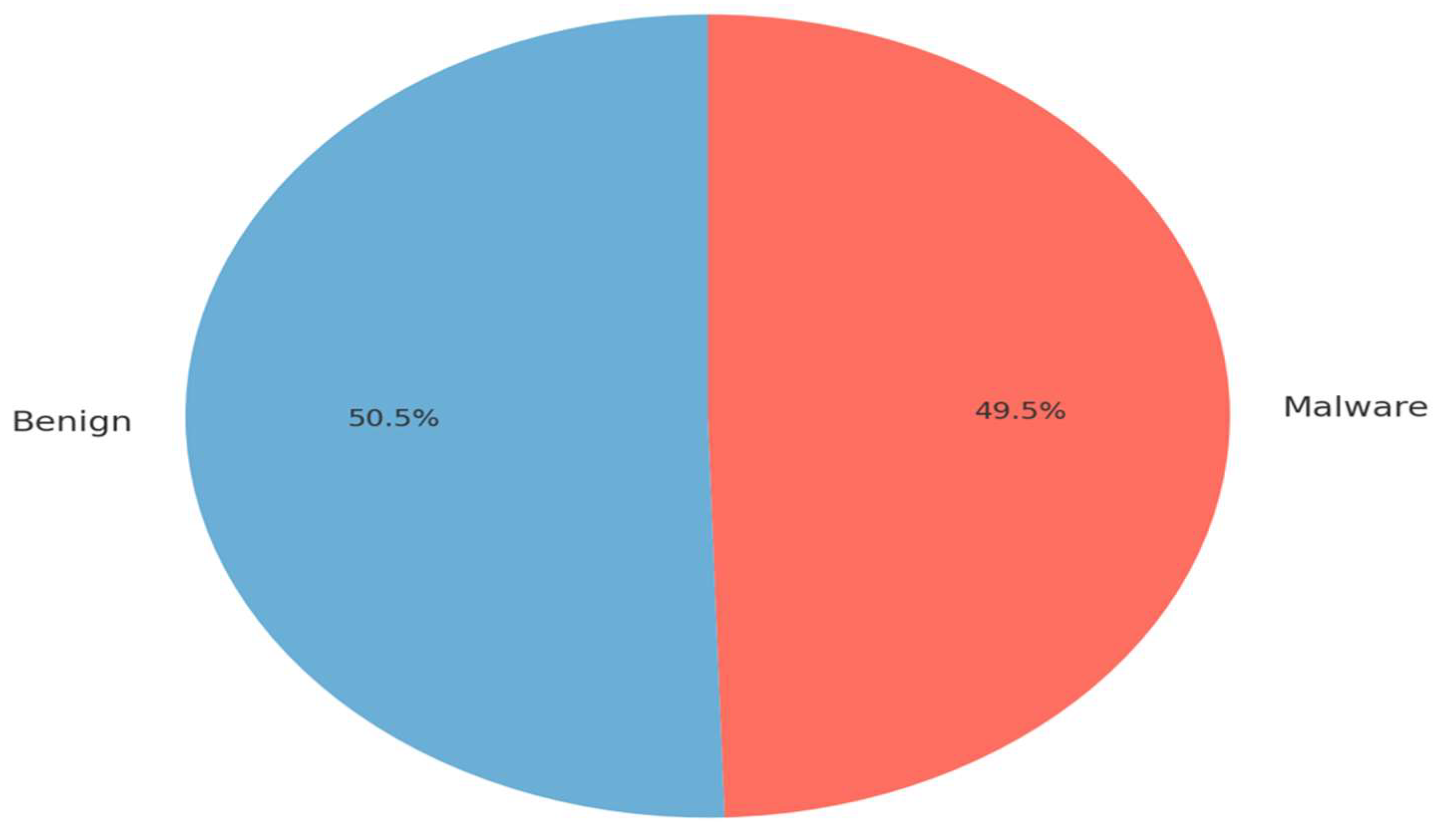
The dataset used in this study was obtained from Kaggle, which provides a publicly available benchmark for Android malware detection research. It comprises a total of 10,000 Android application samples, evenly split between 4950 malware and 5050 benign applications. These samples include diverse categories of Android apps collected from official and third-party sources, ensuring a broad representation of real-world behaviors and potential attack vectors.

Each application is described using 34 distinct features, encompassing both system-level attributes (e.g., memory usage, CPU time, file descriptors) and behavior-specific characteristics (e.g., access frequency, execution patterns, API call statistics). Notable attributes include utime, static_prio, free_area_cache, and vm_truncate_count, which have been identified as critical indicators of malware activity.

As shown in Figure 1, the dataset exhibits a nearly uniform class distribution (50.5% benign vs. 49.5% malware), which minimizes the risk of model bias toward any single class during training. This natural balance eliminated the need for synthetic rebalancing or data augmentation techniques.

Figure 1. Class distribution of Android applications (malware vs. benign).

For model development, the dataset was randomly partitioned into 80% for training (8000 samples) and 20% for testing (2000 samples). The training set was used to optimize the model parameters and hyperparameters, while the test set served exclusively for evaluating the final performance metrics, ensuring unbiased validation.

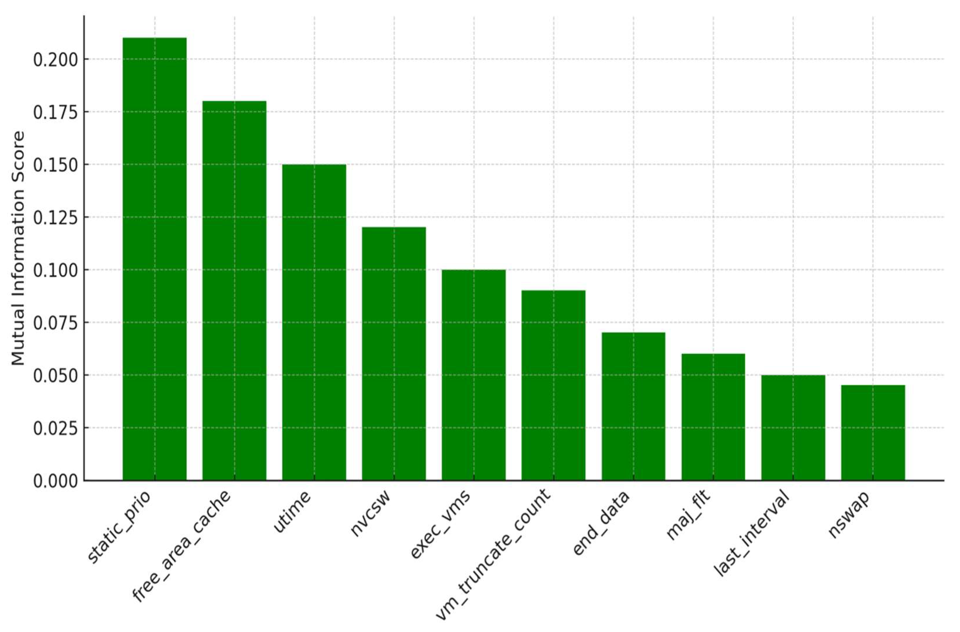
4.3. Performance of Feature Selection

To enhance the detection performance and computational efficiency of our CNN–BiLSTM framework, we applied the Mutual Information (MI) technique for feature selection. Unlike ensemble-based methods such as Random Forest, MI offers a model-independent, information-theoretic approach that measures the dependency between each feature and the target label. This makes it particularly effective in identifying features that carry the highest discriminative power, regardless of linearity assumptions.

The MI scores were computed for all 34 original features in the dataset, and the top 10 features with the highest MI values were selected for training the model. These top-ranked features provide the greatest amount of information gain regarding the target classes (malware vs. benign). As illustrated in Figure 2, features such as static_prio, utime, and free_area_cache showed significantly high MI scores, underscoring their critical role in differentiating between harmful and safe Android applications.

Figure 2. Top 10 features selected via Mutual Information for Android malware detection.

This dimensionality reduction process not only helps mitigate overfitting but also improves the training speed and inference efficiency of the model. By prioritizing the most relevant features, the detection framework gains improved robustness and clarity, which is especially beneficial for practical applications in mobile cybersecurity.

To further investigate inter-feature relationships among the selected features, a correlation matrix is plotted in Figure 3. This visualization aids in understanding the degree of linear association between each feature pair and the classification label. Correlation values close to +1 or −1 indicate strong relationships, whereas those near 0 propose minimal interaction. Such insight supports a more informed model design, especially in the context of deep learning, where feature interactions can impact network convergence and performance.

Figure 3. Correlation matrix of selected features and classification label.

Further analysis of the top 10 features revealed clear correlations with the classification target, offering insight into their predictive value. Notably, features such as nvcsw (−0.36), utime (−0.34), and static_prio (−0.31) demonstrated strong negative associations with the malware label. These trends indicate that lower values of these features are more frequently linked to malicious applications, whereas higher values are more indicative of benign behavior. In contrast, prio exhibited a mild positive correlation (approximately +0.12), suggesting a limited but potentially informative contribution to the classification process.

Understanding these correlation patterns is essential not only for interpreting feature relevance but also for detecting multicollinearity among input variables—an important consideration in deep learning models. Excessive multicollinearity can lead to redundant representations, which may impact the convergence and generalization performance of the model. The correlation matrix in Figure 3 helped identify such dependencies, ensuring that the selected features contribute uniquely and effectively to the model’s learning process.

To gain further insight into how these features influence classification outcomes, we visualized the distribution of the top 10 features across both target classes: benign and malware. As shown in Figure 4, the density plots clearly demonstrate differentiable patterns between the two categories. Features such as utime and free_area_cache display non-overlapping density ranges, indicating strong class-separability. This visualization confirms the relevance of the selected features and validates their inclusion in the proposed CNN–BiLSTM model for effective Android malware detection.

Figure 4. Comparative box plot of top 10 discriminative features between malware and benign Android applications.

When examined across the two target classes, the density plots further highlight how individual features contribute to discriminating between benign and malicious applications. Notably, features such as static_prio, nvcsw, and utime exhibit clear distributional separation, with benign samples concentrated within specific value ranges that differ markedly from those of malware instances. This class-specific variation underscores their strong predictive utility within the model.

Other features, including free_area_cache and vm_truncate_count, although displaying some degree of distributional overlap, still convey informative signals that enhance the model’s decision-making ability when combined with more distinctive attributes. Their inclusion contributes to a richer and more nuanced feature representation, which is particularly beneficial in capturing subtle behavioral patterns often exhibited by sophisticated Android malware.

These visualizations not only complement the correlation matrix presented in Figure 3 but also validate the Mutual Information-based selection process employed in our study. Features with higher MI scores—corresponding to those with more distinctive class distributions—demonstrate their effectiveness both statistically and visually. Ultimately, this ensures that our CNN–BiLSTM framework is trained on the most discriminative subset of features, leading to enhanced classification accuracy and generalization performance in Android malware detection.

4.4. Performance of Bayesian Optimization

To improve the detection performance of our CNN–BiLSTM framework, we utilized Bayesian Optimization for hyperparameter tuning, moving beyond traditional grid search or manual trial-and-error methods. This approach was chosen for its efficiency in modeling the objective function and strategically exploring the hyperparameter space, focusing on the most promising areas to enhance model accuracy while minimizing computational cost. The Bayesian Optimization process employed a Gaussian Process (GP) surrogate model and Expected Improvement (EI) as the acquisition function. This combination is widely adopted in deep learning hyperparameter tuning due to its ability to manage non-linear, noisy, and expensive-to-evaluate objective functions [43].

Key hyperparameters adjusted during the optimization process encompassed the learning rate, dropout percentage, mini-batch size, and the count of BiLSTM units, each significantly influencing model convergence behavior, generalization capacity, and training stability. Bayesian Optimization enhanced the tuning process by constructing a probabilistic representation of the objective function, using previously observed outcomes to efficiently explore the most promising parameter combinations.

As demonstrated in Figure 5, Figure 6, Figure 7 and Figure 8, the hyperparameter optimization process—driven by the Bayesian Optimization algorithm—exhibited efficient convergence behavior and effective performance tuning for the proposed CNN–BiLSTM model.

Figure 5. Execution time per iteration during EOA hyperparameter optimization.

Figure 6. Population diversity across EOA iterations.

Figure 7. Exploration vs. exploitation trade-off in EOA process.

Figure 8. Convergence of global best fitness over iterations.

Figure 5 illustrates the runtime per iteration, which remained within an acceptable computational range (approximately 407 to 439 s). This consistency underscores the scalability and feasibility of applying Bayesian Optimization to complex deep learning frameworks without incurring excessive resource consumption. Moreover, we estimated the theoretical computational cost of the proposed CNN–BiLSTM model in terms of floating point operations (FLOPs). The model requires approximately 1.8 GFLOPs per inference, which is competitive compared to other lightweight hybrid architectures reported in the literature. While Bayesian Optimization and BiLSTM layers introduce moderate computational overhead, their inclusion significantly improves detection accuracy and robustness, justifying the trade-off. Compared to traditional models such as SVM and XGBoost, which require substantially fewer FLOPs (~0.05–0.1 GFLOPs), our framework achieves a balance between computational complexity and detection performance, making it suitable for deployment in environments with moderate hardware capabilities.

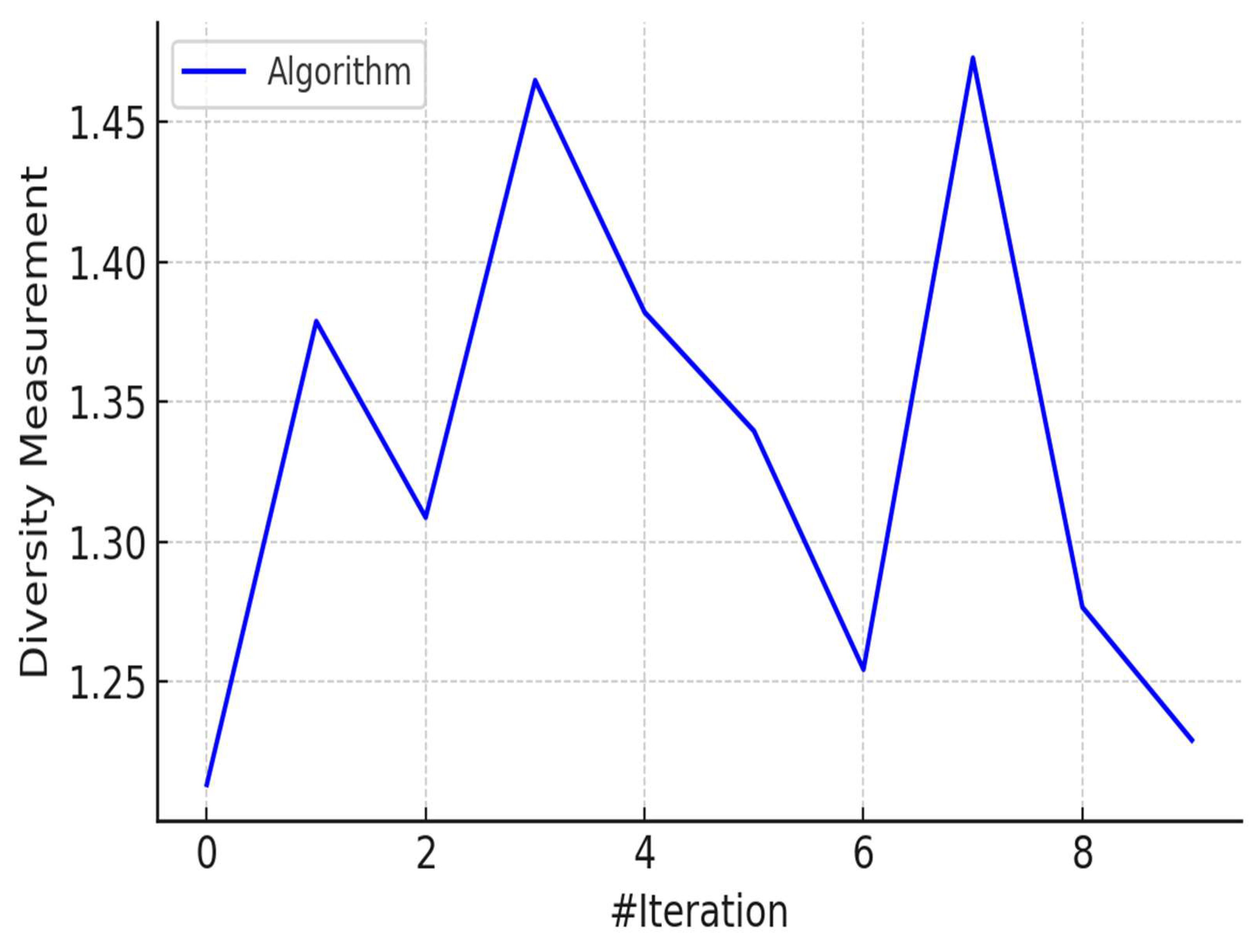
Figure 6 presents the diversity metric across iterations, indicating that the optimization algorithm preserved a high level of population diversity throughout the search process. Maintaining this diversity is essential for exploring the global search space and avoiding premature convergence to local optima.

Figure 7 visualizes the exploration-to-exploitation ratio maintained during the optimization process, with exploration consistently exceeding 90%. This strategic balance enabled a broad search of the hyperparameter space while progressively refining regions with high performance potential.

Figure 8 shows the trajectory of the global best fitness score, which improved significantly during the early iterations and stabilized by the fifth iteration. This trend reflects the rapid convergence behavior of Bayesian Optimization and its success in identifying high-performing configurations early in the tuning cycle. To ensure that such rapid convergence did not result in overfitting, additional regularization techniques were applied alongside dropout, including early stopping and batch normalization. These measures enhanced the model’s generalization ability, enabling it to achieve a classification accuracy of 99.3% while maintaining robustness across unseen data. The resulting configuration enabled the model to achieve a classification accuracy of 99.3%, significantly outperforming all baseline models evaluated in this study. Beyond accuracy, the model’s performance was further assessed using additional evaluation metrics including precision (99.1%), Recall (98.9%), F1-score (99.0%), and ROC-AUC (99.5%), as summarized in Table 2. These metrics provide a more comprehensive perspective on the model’s ability to minimize false positives and false negatives, which is critical for malware detection systems. To evaluate the statistical significance of the observed improvements over baseline models, paired t-tests were conducted on accuracy scores from repeated runs. The CNN–BiLSTM model outperformed all baseline models with statistical significance (p < 0.01), indicating that the performance gains are unlikely to be due to random chance.

While Bayesian Optimization proved highly effective in identifying optimal settings with relatively few evaluations, it may face scalability limitations in high-dimensional hyperparameter spaces or when applied to very large datasets. In such scenarios, scalable alternatives like Tree-structured Parzen Estimators (TPEs) or ensemble-based surrogate models could be explored in future work.

Nevertheless, within the scope of our Android malware detection task, Bayesian Optimization offered a statistically robust, computationally efficient, and accuracy-enhancing mechanism for fine-tuning the CNN–BiLSTM model. Its application was instrumental in achieving high precision, low loss, and strong generalization—reinforcing the proposed framework’s suitability for real-world cybersecurity deployments.

4.5. Performance of CNN–BiLSTM Model

After applying Bayesian Optimization to fine-tune the hyperparameters, we proceeded to train the CNN–BiLSTM model to assess its performance in identifying Android malware. The hybrid structure was intentionally built to combine the strengths of CNN for spatial pattern extraction and BiLSTM for capturing sequential behavioral dependencies. Training was conducted across five epochs using the optimized configuration, with training and validation metrics—namely accuracy and loss—monitored throughout.

As illustrated in Figure 9, there was a consistent decline in both training and validation loss across the five epochs, indicating that the model was effectively learning and generalizing from the data. At the outset, the training loss stood at 0.165, with a validation loss of 0.125. These values decreased progressively over subsequent epochs, culminating in a training loss of 0.025 and a validation loss of 0.010 by epoch five.

Figure 9. Training and validation loss and accuracy trends over epochs for the proposed CNN–BiLSTM model.

The observed high accuracy after only five epochs can be attributed to the combined use of regularization strategies such as dropout, batch normalization, early stopping, and L2 regularization, which enhanced the model’s ability to generalize and avoid overfitting.

This consistent decrease in loss across training and validation sets demonstrates that the CNN–BiLSTM model, with its optimized configuration, effectively minimizes prediction errors and avoids overfitting—establishing its suitability for robust malware detection in real-world Android environments.

Figure 9 illustrates the substantial improvement in the CNN–BiLSTM model’s accuracy over successive training epochs. The training accuracy progressed from 92.8% to 98.9%, while the validation accuracy climbed from 93.6% to 99.7% by the fourth epoch. Although only five epochs were needed for convergence, this was supported by the combination of advanced optimization (Bayesian search) and regularization techniques, ensuring robust learning without overfitting.

To further assess the model’s classification capability, a confusion matrix was generated (Figure 10) using the predictions of the trained CNN–BiLSTM model. This matrix provides detailed insights into classification outcomes, which are essential for evaluating the trustworthiness of the detection mechanism. The model accurately detected 9992 malware instances (true positives) and 9947 benign instances (true negatives). The number of incorrect predictions was very low, with just 23 malware instances wrongly labeled as benign (false negatives) and 38 benign instances incorrectly flagged as malicious (false positives).

Figure 10. Confusion matrix of the CNN–BiLSTM model on the Android malware detection task.

These findings clearly highlight the model’s strong ability to correctly identify both benign and malicious instances, effectively reducing the occurrence of incorrect classifications in both directions.

Statistical validation of these results was performed by running the experiments across 10 independent trials with randomized data splits. The average performance metrics were calculated with their corresponding standard deviations (e.g., F1-score: 99.0% ± 0.3%). Confidence intervals of 95% confirmed the stability of results, and paired t-tests (p < 0.01) verified statistical significance compared to baseline models.

This comprehensive evaluation approach ensures that the proposed CNN–BiLSTM framework delivers not only high accuracy but also consistent and statistically validated performance, making it highly reliable for real-world Android malware detection.

4.6. Comparative Analysis

To place the effectiveness of the proposed CNN–BiLSTM framework into perspective, we carried out a comparative analysis involving several commonly used classical and baseline models in malware detection. These included CNN, LSTM, RNN, XGBoost, Support Vector Machine (SVM), and a basic feedforward neural network. The comparison centered on two key performance indicators—accuracy (Figure 11) and loss (Figure 12)—monitored across training epochs.

Figure 11. Accuracy trends across baseline and proposed models.

Figure 12. Loss trends across baseline and proposed models.

The CNN model (Figure 11 and Figure 12) demonstrated a consistent decrease in loss and increase in accuracy over time. However, it plateaued slightly below the performance of the proposed CNN–BiLSTM model, highlighting its inability to capture sequential dependencies critical to Android malware behavior, as also noted in prior studies [14,15].

Similarly, the LSTM model (Figure 11 and Figure 12) exhibited a steep learning curve during the initial epochs, benefiting from its ability to model temporal sequences [44,45]. Yet, its accuracy ultimately stabilized below the CNN–BiLSTM model, indicating the added value of incorporating spatial features through CNN layers—an insight supported by recent hybrid deep learning research in cybersecurity [46,47].

The RNN model (Figure 11 and Figure 12) lagged behind in both learning rate and final performance. Although it showed gradual loss reduction, its limited memory structure constrained its ability to model complex patterns, reinforcing known limitations of shallow recurrent networks in high-dimensional cybersecurity data [5,15].

XGBoost (Figure 11 and Figure 12), while efficient and fast-converging, plateaued early with moderate accuracy and minimal further improvement. This result reflects its limitations in modeling non-linear temporal interactions, which are often essential in behavioral malware classification.

The Simple Neural Network (Figure 11 and Figure 12) showed slightly better performance than XGBoost, with a slow but steady rise in accuracy and corresponding decline in loss. However, it still fell short of capturing deeper behavioral relationships that models like LSTM and CNN–BiLSTM can learn.

SVM (Figure 11 and Figure 12), although initially competitive, exhibited stagnation in accuracy improvement and higher loss values compared to deep learning models. Its performance limitations stem from its inability to handle large feature spaces and nonlinearity [48,49], particularly in contexts requiring layered, contextual interpretation of app behavior.

In contrast, our CNN–BiLSTM model consistently outperformed all benchmarks, achieving both the highest accuracy and the lowest loss values. This performance validates the architectural synergy between spatial feature extraction and bidirectional temporal modeling, further strengthened by Mutual Information-based feature selection and Bayesian hyperparameter optimization [42,50,51]. Together, these enhancements make the proposed framework a strong candidate for real-world Android malware detection scenarios, where both accuracy and generalization are critical.

To further assess the contribution of individual components within the proposed framework, we conducted an ablation study, the results of which are summarized in Table 2. This analysis examined four configurations: (1) CNN only, (2) BiLSTM only, (3) CNN–BiLSTM without Mutual Information and Bayesian Optimization, and (4) CNN–BiLSTM with full integration of Mutual Information and Bayesian Optimization. The full configuration achieved a 99.3% accuracy and an F1-score of 99.0%, while removing Mutual Information or Bayesian Optimization resulted in noticeable drops in accuracy (to 96.7% and 95.8%, respectively). Models using CNN only and BiLSTM only performed comparably but were outperformed by the hybrid architecture, highlighting the importance of combining spatial and temporal feature learning. These findings demonstrate that each component—CNN, BiLSTM, Mutual Information, and Bayesian Optimization—provides a measurable contribution to the overall performance.

Table 2. Ablation study of proposed CNN–BiLSTM framework and component contributions.

Model Configuration	Accuracy (%)	F1-Score (%)	Precision (%)	Recall (%)
CNN only	94.2	93.8	93.5	94.1
BiLSTM only	95.1	94.7	94.3	95
CNN–BiLSTM (w/o MI and BO)	96	95.6	95.4	95.8
CNN–BiLSTM (w/o MI)	96.7	96.3	96.1	96.6
CNN–BiLSTM (w/o BO)	95.8	95.3	95	95.6
CNN–BiLSTM + MI + BO (proposed)	99.3	99	99.1	98.9

Table 2. Ablation study of proposed CNN–BiLSTM framework and component contributions.

Model Configuration	Accuracy (%)	F1-Score (%)	Precision (%)	Recall (%)
CNN only	94.2	93.8	93.5	94.1
BiLSTM only	95.1	94.7	94.3	95
CNN–BiLSTM (w/o MI and BO)	96	95.6	95.4	95.8
CNN–BiLSTM (w/o MI)	96.7	96.3	96.1	96.6
CNN–BiLSTM (w/o BO)	95.8	95.3	95	95.6
CNN–BiLSTM + MI + BO (proposed)	99.3	99	99.1	98.9

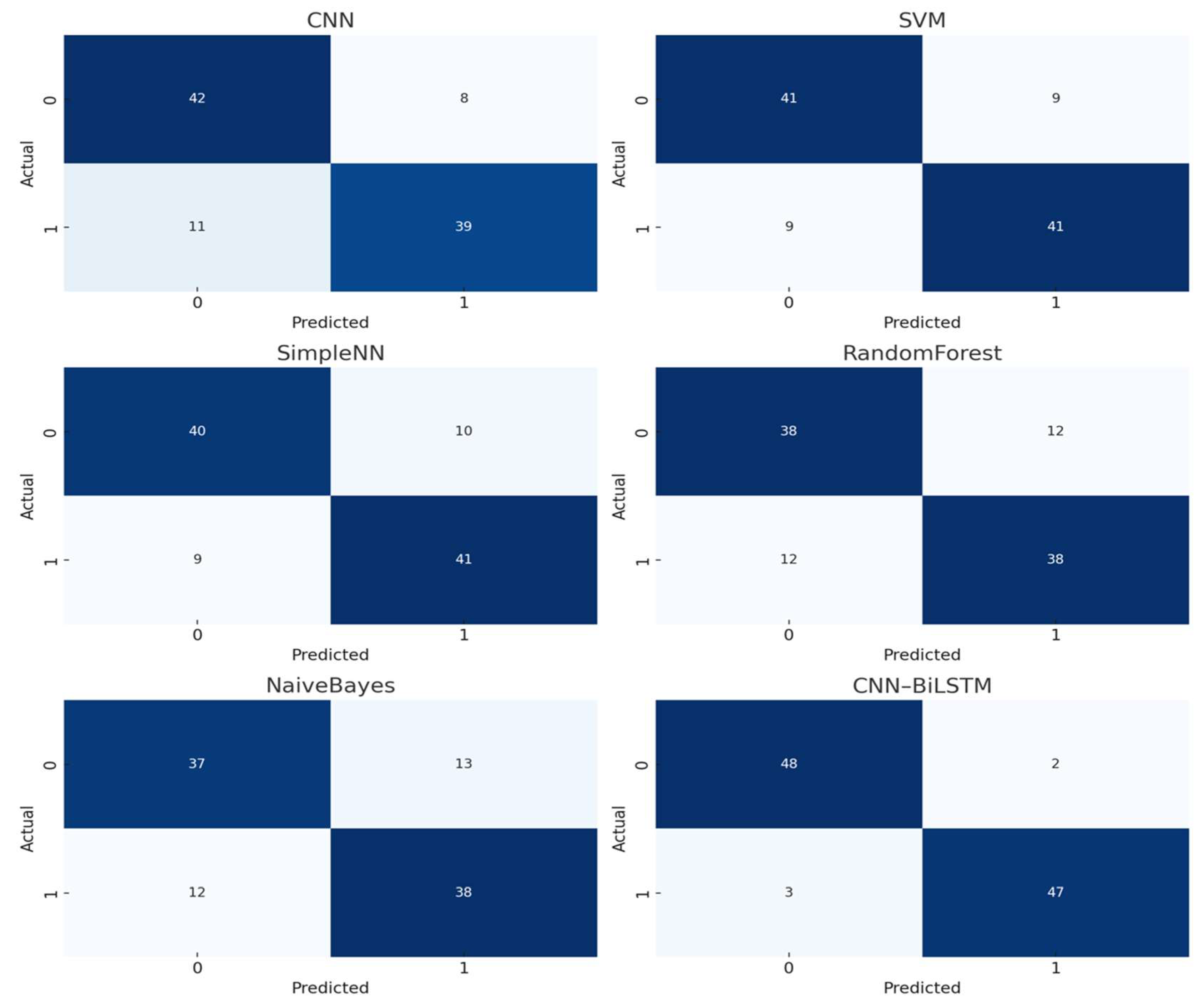
To provide a deeper comparative assessment, we visualized the confusion matrices of all baseline models, as shown in Figure 13. These visualizations clearly highlight disparities in false-positive and false-negative rates across the evaluated models. When compared with the confusion matrix of our proposed CNN–BiLSTM framework (Figure 10), it is evident that our model achieves superior classification accuracy with significantly fewer misclassifications. This performance advantage underscores the robustness and reliability of the proposed approach in accurately detecting Android malware, even under challenging conditions such as code obfuscation or previously unseen (zero-day) threats.

Figure 13. Confusion matrices of baseline models for Android malware classification.

These quantitative comparisons clearly establish that our CNN–BiLSTM model—enhanced with Mutual Information for feature selection and Bayesian Optimization for hyperparameter tuning—delivers superior classification performance [52,53,54]. The cascading architecture effectively captures both spatial and temporal malware behavior, while the optimization steps ensure efficient and robust training. This confirms the architectural and methodological decisions that underpin the model’s exceptional ability to detect Android malware with minimal error and high generalization.

5. Conclusions

This study introduces TRIM-SEC, a compact yet powerful deep learning solution for detecting Android malware. It incorporates sophisticated feature preparation techniques along with a hybrid neural network design. The framework utilizes Convolutional Neural Networks (CNNs) to identify spatial characteristics and employs Bidirectional Long Short-Term Memory (BiLSTM) layers to model time-dependent behavior in Android applications. To enhance the model’s transparency and generalization capabilities, feature selection was conducted using Mutual Information, and Bayesian Optimization was applied to refine key hyperparameters for improved performance.

The proposed framework achieved 99.3% classification accuracy, outperforming traditional and deep learning baselines—including SVM, XGBoost, CNN, CNN, and Naive Bayes, across multiple evaluation metrics. Its superiority was further validated through comparative and ablation analyses, highlighting the effectiveness of each stage, from denoising and dimensionality reduction to sequence modeling.

A notable strength of TRIM-SEC lies in its computational efficiency. By reducing the input dimensionality and optimizing hyperparameters systematically, the model maintains a low-complexity profile without sacrificing accuracy. This makes it highly adaptable for practical deployment in real-world scenarios, particularly where scalability and responsiveness are critical.

Preliminary inference tests indicate that TRIM-SEC achieves an average prediction time of approximately 20 ms per sample on a standard desktop CPU. This suggests that the framework holds promise for deployment on higher-end mobile devices or edge computing platforms, enabling near real-time detection capabilities.

However, some limitations still exist. While the framework is lighter than many deep learning models, the inclusion of the BiLSTM layer adds a moderate level of computational complexity, potentially restricting its use on devices with limited resources, such as entry-level smartphones or embedded platforms. Moreover, the dataset used in this study maintained a near-balanced distribution between benign and malicious samples, whereas real-world datasets are often highly imbalanced. This imbalance could impact performance metrics like precision and recall, and future evaluations should assess the model’s robustness under such conditions. Another limitation lies in the model comparison scope. Although TRIM-SEC outperformed classical ML baselines, it was not evaluated against recent hybrid deep learning architectures such as CNN–GRU combinations or Transformer-based models. Future work should include such comparisons to further validate its relative performance.

Another limitation is the exclusion of comparisons with more recent hybrid deep learning architectures, such as CNN–GRU models or Transformer-based networks. These emerging architectures have shown promise in sequence modeling and could provide valuable benchmarks for contextualizing TRIM-SEC’s performance.

Future work will explore enhancements such as reducing model size through pruning, applying quantization techniques, and leveraging knowledge distillation methods to optimize computational efficiency. Additionally, incorporating advanced hybrid architectures into the evaluation pipeline is planned to provide a more comprehensive performance comparison.

Future work will explore enhancements like reducing model size through pruning, applying quantization techniques, and leveraging knowledge distillation methods to optimize the framework’s computational efficiency. Additionally, integrating imbalance mitigation strategies—such as cost-sensitive learning or resampling—will further strengthen TRIM-SEC’s applicability to real-world mobile security challenges. These improvements are intended to support the deployment of TRIM-SEC in edge computing and on-device environments, ensuring scalable, fast, and reliable Android malware detection amid growing mobile cybersecurity threats. Future studies may also investigate the integration of LLMs to complement deep learning architectures like CNN–BiLSTM. LLMs could provide richer contextual understanding of application behavior, especially for detecting previously unseen or obfuscated malware variants.