Supply Chain Design Method for Introducing Floating Offshore Wind Turbines Using Network Optimization Model

Abstract

This paper presents a method to model and optimize the supply chain processes for floating offshore wind turbines using a network model based on Generalized Multi-Commodity Network Flows (GMCNF). The proposed method represents production bases, base ports, installation sites, component transfer areas, and transportation routes as nodes and arcs within the network. The installation process is modeled using three transport concepts: assembling components at the base port, direct assembly and installation at the installation site, and transferring components to the installation vessel at a nearby port. These processes are expressed as a linear network model, with the objective function set to minimize total transportation and assembly costs. The optimal transportation network is derived by solving the network problem while incorporating constraints such as supply, demand, and transportation capacity. Case studies demonstrate the method’s effectiveness in optimizing the supply chain and evaluating potential new production site locations for floating foundations, considering overall supply chain optimization.

1. Introduction

Due to the recent global warming issue, the large-scale adoption of renewable energy is being promoted worldwide [1]. Wind power generation is one of the key components of renewable energy, and various efforts are underway to facilitate its large-scale deployment, both onshore and offshore. The large-scale deployment of offshore wind power generation is planned in many parts of the world, accompanied by a trend toward larger wind turbine sizes [2]. Typically, the optimal wind turbine type for a specific location is determined through analysis of annual wind profiles and relevant meteorological conditions [3]. Due to the inherent uncertainty of wind conditions [4], it is essential to assess the potential of wind power projects based on extensive datasets and appropriate probabilistic distribution models [5,6].

In addition, careful consideration must be given to selecting the most economical, efficient, and reliable turbine to maximize performance and minimize costs including supply chain [7]. Establishing a supply chain is essential for the large-scale introduction of offshore wind power, and several related studies have been conducted. Akbari et al. [8] used hierarchical analysis to determine the factors that are important in selecting base ports for offshore wind farms. Prostean et al. [9] used hierarchical analysis to identify risk factors in the supply chain of offshore wind farms. Several studies have been conducted on supply chain development for offshore wind turbine installation phases. Sarker et al. [10] calculated the cost of installing wind turbines when varying the output of each turbine when building an offshore wind farm of a given output. Kaiser et al. [11] and Ahn et al. [12] developed an installation model considering four types of vessels and calculated and compared the cost and duration of offshore wind farm installation in Korea. Vis et al. [13] developed a model to optimize the assembly and installation of wind turbines taking into account weather conditions and calculated the cost and duration of wind turbine installation in the North Sea. Barlow et al. [14] developed a weather-aware installation model using discrete event simulation and robust optimization, which was used for decision making for an offshore wind farm project in the UK.

While these papers have performed detailed modeling and evaluation of installing offshore wind turbine projects, they are concerned only with bottom-fixed offshore wind turbines in one site. This paper focuses on the supply chain for installing floating offshore wind turbines, which will be increasingly commercialized and deployed. Floating offshore wind power offers access to higher wind speeds and broader deployment areas than onshore systems, but its cost remains significantly higher. Although it becomes more economically favorable than fixed-bottom structures beyond certain depths, overall viability declines with increasing depth and distance from shore, and design standardization has yet to be achieved [15]. However, in the context of the expansion of renewable energy deployment, the adoption of floating offshore wind turbines will be essential after the saturation of installations of fixed-bottom wind turbines [16]. In general, floating offshore wind farm projects conduct a life cycle analysis of target offshore wind farms using a cost breakdown structure, and the life cycle cost system developed takes into account different phases [17] on the basis of the levelized cost of energy (LCOE) [18]. In recent years, there has been a growing body of research not only on the post-installation evaluation of wind farms but also on the supply chain processes prior to installation, with particular attention paid to logistics and transportation [10]. Hasumi et al. [19] focused their analysis on the time required for the development and installation of wind farms. Poulsen and Lema [20] identified that key bottlenecks exist in logistics in Europe and China. Kruger et al. [21] examined key factors and experiences from two floating offshore wind projects to analyze how they shape the development of a reliable and sustainable supply chain essential for large-scale deployment in the context of global decarbonization goals. González et al. [22] proposed a conceptual framework to optimize offshore wind farm installation costs by structuring key logistical decisions such as port and vessel selection, the installation strategy, and scheduling. Since the floating offshore wind turbine business is still in its infancy, it is necessary to design a strategy to introduce floating offshore wind turbines that covers the entire process from production to transportation of components and wind turbine assembly and installation [23].

This paper aims to develop a supply chain design method for introducing floating offshore wind turbines using a network optimization model. A supply chain for the introduction of floating offshore wind turbines, including a series of processes from component transportation, wind turbine assembly, and installation, is represented by a network model. A model-based supply chain design method for introducing floating offshore wind turbines is developed through network optimization technology. The primary contribution of this paper lies in proposing a comprehensive supply chain optimization approach for the installation of floating offshore wind turbines by leveraging the network optimization framework.

2. Proposed Method

Figure 1 illustrates the proposed methodology. The process begins by registering candidate base locations as nodes and assigning demand and supply data to each one. It then models all possible supply chain configurations as a network, including transportation capacity constraints for each arc. Finally, it solves a transportation cost minimization problem by identifying the optimal supply chain configuration using a network optimization technique.

The proposed method models these three supply chain concepts according to the Generalized Multi-Commodity Network Flows (GMCNF) model [24]. The GMCNF framework extends conventional network flow formulations by introducing three distinct types of matrix operations—requirement, transformation, and concurrency—and by generalizing the network structure to permit loop edges at nodes (graph loops) as well as multiple edges between the same pair of nodes (multigraph). These extensions enable the representation of multiple interacting commodities, with interdependencies formulated as requirements at nodes, transformations along edges, and concurrent flows within edges. Based on the GMCNF framework, this paper employs three concepts, the “base port concept”, “offshore feeder-ship concept”, and “base port feeder-ship concept”, as a series of flows from the production of each component to the installation of the floating offshore wind turbine in the target sea area, referring to the paper by Ait-Alla et al. [25]. Specifically, production bases, component transfer areas, base ports, and installation sites are modeled as nodes, and the processes of transportation and assembly are modeled as arcs. Here, the proposed method needs the supply and demand information related to the offshore wind turbine installation in the supply chain and the relationships among all the nodes and arcs in the candidate supply chain concepts as input information.

Finally, the proposed method can calculate the optimal supply chain plan by solving a linear programming problem, with the lowest total cost as the objective function.

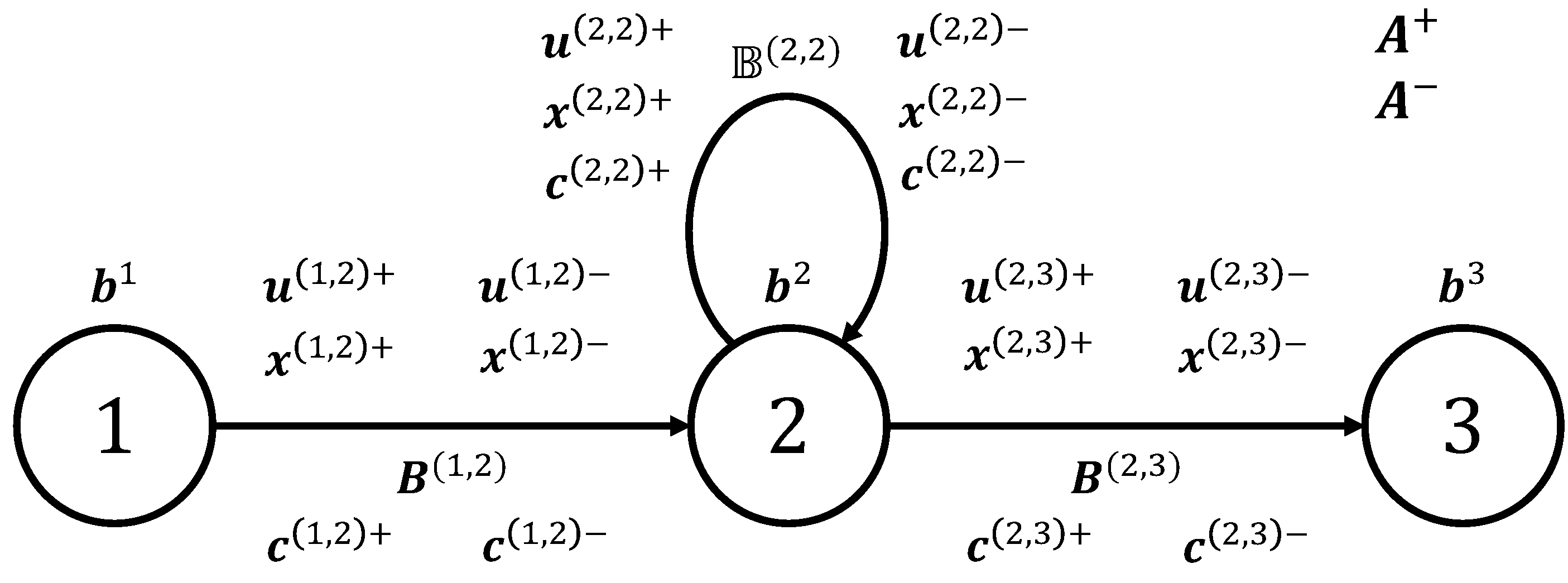
2.1. Supply Chain Modeling

This paper models the supply chain of a floating offshore wind turbine installation according to the GMCNF model [24]. This paper assumes that all floating wind turbines being installed are the same in the target supply chain, and one floating wind turbine consists of members with one tower, three blades, one nacelle, and one floating foundation.

$\mathcal{N}$ represents the set of all nodes, and $\mathcal{A}$ represents the set of all arcs. ${\mathcal{A}}_{\mathrm{transportation}}$ represents the set of all transportation arcs and ${\mathcal{A}}_{\mathrm{assembly}}$ represents the set of all assembly arcs. In this paper, $a=(i,j)$ shows that directed arc a connects from node i to node j. The side adjacent to node i in a is the head, and the side adjacent to node j in a is the tail. Equation (1) defines ${\mathit{A}}^{+}$ and ${\mathit{A}}^{-}$, which represent the incidence matrices of the network model. Only the heads of arcs are considered in ${\mathit{A}}^{+}$, and only the tails of arcs are considered in ${\mathit{A}}^{-}$. Equations (2) and (3) define the elements of node $i\in \mathcal{N}$ and arc $a=(j,k)\in \mathcal{A}$ in ${\mathit{A}}^{+}$ and ${\mathit{A}}^{-}$.

$${\mathit{A}}^{\pm }=\left[A_{i,a=(j,k)}^{\pm }\right]\{i,j,k\}\in \mathcal{N},a\in \mathcal{A}$$

(1)

$$A_{i,a=(j,k)}^{+}=\left\{\begin{array}{cc}1\hfill & \mathrm{if}i=j\hfill \\ 0\hfill & \mathrm{otherwise}\hfill \end{array}\right.$$

(2)

$$\begin{array}{c}{A}_{i,a=(j,k)}^{-}=\left\{\begin{array}{cc}1\hfill & \mathrm{if}i=k\hfill \\ 0\hfill & \mathrm{otherwise}\hfill \end{array}\right.\end{array}$$

(3)

Figure 2 shows an example network model of a supply chain consisting of a production base, an assembly site, and an installation site, each at one location. In Figure 2, node 1 represents the production base, node 2 represents the assembly site, and node 3 represents the installation site. In Figure 2, these are defined as $\mathcal{N}=\{1,2,3\}$, $\mathcal{A}=\left\{\right(1,2),(2,2),(2,3\left)\right\}$, ${\mathcal{A}}_{\mathrm{transportation}}=\{(1,2),(2,3)\}$, and ${\mathcal{A}}_{\mathrm{assembly}}=\left\{(2,2)\right\}$. The incidence matrices ${\mathit{A}}^{+}$ and ${\mathit{A}}^{-}$ of Figure 2 are defined as in Equation (4). The order of rows and columns in each incidence matrix corresponds to the orders of $\mathcal{N}$ and $\mathcal{A}$, respectively.

$${\mathit{A}}^{+}=\left[\begin{array}{ccc}1& 0& 0\\ 0& 1& 1\\ 0& 0& 0\end{array}\right],{\mathit{A}}^{-}=\left[\begin{array}{ccc}0& 0& 0\\ 1& 1& 0\\ 0& 0& 1\end{array}\right]$$

(4)

Nodes have each component’s supply and demand attributes related to the target floating wind turbines. ${\mathit{b}}^i$ represents the magnitude of supply and demand of each node $i\in \mathcal{N}$. Equation (5) shows the definition of ${\mathit{b}}^i$. Each element of ${\mathit{b}}^i$ is each component’s supply and demand at node i. In the proposed method, we should register ${\mathit{b}}^i$ considering each node’s supply and demand information. In general, when modeling the supply chain of a floating offshore wind turbine installation, the demand for floating wind turbines is registered only at the installation site nodes as minus values of $b_{\mathrm{product}}^i$, which express the demand of floating wind turbines as the final product and have zero values for other elements. The supply of each component of a floating wind turbine is registered only at the production base nodes as $b_{\mathrm{product}}^i=0$ and other elements have positive values. The assembly nodes are registered with ${\mathit{b}}^i=\mathbf{0}$ because there is no demand or supply at the assembly base.

$${\mathit{b}}^i={\left(b_{\mathrm{tower}}^i,b_{\mathrm{blade}}^i,b_{\mathrm{nacelle}}^i,b_{\mathrm{foundation}}^i,b_{\mathrm{product}}^i\right)}^{\mathsf{T}}i\in \mathcal{N}$$

(5)

Arcs have each component’s transportation amount, transportation capacity, transportation cost, and flow transportation matrix attributes related to the target floating wind turbines. ${\mathit{x}}^{a\pm }$ expresses the amount of transportation of each component on arc $a\pm \in \mathcal{A}$. Equation (6) shows the definition of ${\mathit{x}}^{a\pm }$. ${\mathit{u}}^{a\pm }$ expresses the transportation capacity of each component on arc $a\pm \in \mathcal{A}$. Equation (7) shows the definition of ${\mathit{u}}^{a\pm }$. ${\mathit{c}}^{a\pm }$ expresses the transportation cost of each component on arc $a\pm \in \mathcal{A}$. Equation (8) shows the definition of ${\mathit{c}}^{a\pm }$.

$${\mathit{x}}^{a\pm }={\left(x_{\mathrm{tower}}^{a\pm },x_{\mathrm{blade}}^{a\pm },x_{\mathrm{nacelle}}^{a\pm },x_{\mathrm{foundation}}^{a\pm },x_{\mathrm{product}}^{a\pm }\right)}^{\mathsf{T}}a\in \mathcal{A}$$

(6)

$${\mathit{u}}^{a\pm }={\left(u_{\mathrm{tower}}^{a\pm },u_{\mathrm{blade}}^{a\pm },u_{\mathrm{nacelle}}^{a\pm },u_{\mathrm{foundation}}^{a\pm },u_{\mathrm{product}}^{a\pm }\right)}^{\mathsf{T}}a\in \mathcal{A}$$

(7)

$${\mathit{c}}^{a_{\pm }}={\left(c_{\mathrm{tower}}^{a\pm },c_{\mathrm{blade}}^{a\pm },c_{\mathrm{nacelle}}^{a\pm },c_{\mathrm{foundation}}^{a\pm },c_{\mathrm{product}}^{a\pm }\right)}^{\mathsf{T}}a\in \mathcal{A}$$

(8)

${\mathit{B}}^a$ expresses the flow transportation matrix of each component on arc $a\in \mathcal{A}$. The flow transportation matrix is a matrix that expresses the ratio of the amount of each component transported to the amount of each component transported. In this proposed method, ${\mathit{B}}^a$ works to transfer ${\mathit{x}}^{a+}$ to ${\mathit{x}}^{a-}$ on arc a. Equations (9) and (10) show the definition of ${\mathit{B}}^a$ in this paper. The transport arc is set as an identity matrix $\mathit{I}$ since it does not change the state of the transport target, as in Equation (9). Assuming a floating wind turbine consisting of one tower, three blades, one nacelle, and one floating foundation, the flow transformation matrix of an assembly arc is set as shown in Equation (10).

$${\mathit{B}}^a=\mathit{I}\forall a\in {\mathcal{A}}_{\mathrm{transportation}}$$

(9)

$${\mathit{B}}^a=\left[\begin{array}{ccccc}0& 0& 0& 0& 0\\ 0& 0& 0& 0& 0\\ 0& 0& 0& 0& 0\\ 0& 0& 0& 0& 0\\ {\displaystyle \frac{1}{4}}& {\displaystyle \frac{1}{12}}& {\displaystyle \frac{1}{4}}& {\displaystyle \frac{1}{4}}& 1\end{array}\right]\forall a\in {\mathcal{A}}_{\mathrm{assembly}}$$

(10)

2.2. Supply Chain Flow Optimization

In the proposed method, the design variables for the supply chain flow optimization are the transport volumes ${\mathit{x}}^{a\pm }$ of each arc a, shown in Equation (6). This paper sets the objective function as Equation (11), which expresses the sum of the transportation and assembly costs of installing all floating wind turbines at the install sites in the overall process.

$$J=\underset{x^{a\pm }}{min}\sum _{a\in \mathcal{A}}\left({{\mathbf{c}}^{a+}}^{\mathsf{T}}{\mathit{x}}^{a+}+{{\mathbf{c}}^{a-}}^{\mathsf{T}}{\mathit{x}}^{a-}\right)$$

(11)

The proposed method sets the following constraints. Equation (12) shows the mass balance constraint: that the amount of each component transported to each node is equal to the amount of each component transported from each node. Equation (13) shows the transportation capacity constraint: that the amount of each component transported to each arc is within the transportation capacity.

$$\sum _{j:a=(i,j)\in \mathcal{A}}{\mathit{A}}_{i,a}^{+}{\mathit{x}}^{a+}-\sum _{j:a=(j,i)\in \mathcal{A}}{\mathit{A}}_{i,a}^{-}{\mathit{x}}^{a-}\le {\mathit{b}}^i\forall i\in \mathcal{N}$$

(12)

$$0\le {\mathit{x}}^{a\pm }\le {\mathit{u}}^{a\pm }\forall a\in \mathcal{A}$$

(13)

Equation (14) represents the constraint that the state of the components changes during transportation on each arc. When a is an assembly arc, applying Equation (14) when ${\mathit{x}}^{a+}={(1,3,1,1,0)}^{\mathsf{T}}$ results in ${\mathit{x}}^{a+}={(0,0,0,0,1)}^{\mathsf{T}}$. This expresses that the one tower, three blades, one nacelle, and one floating foundation are assembled into one floating wind turbine. Only Equation (14) would allow transportation even when the component proportions of each part were different to those of the target floating wind turbines. In practice, it is natural to perform assembly with each component having no excess or deficiency concerning the product. Equation (15) imposes the constraint that the floating offshore wind turbine’s components have no excess or deficiency in the finished product when each component is entered into the assembly arcs.

$${\mathit{B}}^a{\mathit{x}}^{a+}={\mathit{x}}^{a-}\forall a\in \mathcal{A}$$

(14)

$$x_{\mathrm{tower}}^{a+}={\displaystyle \frac{1}{3}}{x}_{\mathrm{blade}}^{a+}=x_{\mathrm{nacelle}}^{a+}=x_{\mathrm{foundation}}^{a+}\forall a\in {\mathcal{A}}_{\mathrm{assembly}}$$

(15)

2.3. Generating Candidate Supply Chain Proposal

This paper adopts three concepts as the sequence of flow from the production of each component to the installation of the floating offshore wind turbine in the target sea area: the base port concept, the offshore feeder-ship concept, and the base port feeder-ship concept, referring to the paper by Ait-Alla et al. [25]. The base port concept is a transportation method in which each component is transported from the manufacturing facility to the port by carrier ship; the floating wind turbine is assembled at the port and then transported to the installation area by installation ships. The base port feeder-ship concept is a transportation method in which the floating wind turbine is assembled onboard the installation vessel instead of the port that served as the assembly base in the base port concept. The offshore feeder-ship concept is a transportation method in which the components are transported to the installation vessel by feeder ships at the estuary or port near the installation area instead of the port that served as the assembly base in the base port concept. The base port concept represents the standard approach for the installation of floating offshore wind turbines. In contrast, the offshore feeder-ship concept involves transporting the required components directly to the installation site using feeder vessels and conducting the installation offshore. This approach poses greater technical challenges due to the complexity of offshore assembly operations. The base port feeder-ship concept, while similar to the base port concept in terms of logistical aggregation, differs in that the role of the base port—specifically, the consolidation of components—is assumed by the installation vessel itself. Consequently, this results in differences in chartering costs and the duration required for the overall installation process. Note that the concepts proposed by Ait-Alla et al. [25] are treated as candidate configurations within our proposed framework. The method enables comprehensive optimization of all these concepts, allowing the identification of intermediate supply chain configurations that are not limited to the original conceptual boundaries.

When designing the supply chain in this paper, the proposed method first sets up all candidate supply chain proposals exhaustively. Then, optimization calculations are performed according to the objective function in Equation (11) to determine the final candidate supply chain proposal. Since the formulation in this study is linear in scope, the proposed method can calculate the final supply chain proposal quickly using linear programming, even if the number of candidate supply chain proposals is large.

3. Case Studies

This paper applied the proposed method to design supply chains for two simple case studies in Japan. Case A is a network problem where two floating offshore wind turbines are installed in each location. In case B, the proposed method solves the network problem for multiple scenarios, with potential production bases added to the network of case A to confirm the effectiveness of the proposed method in designing a supply chain for introducing and installing floating offshore wind turbines, taking into account various options. This case study considers only the same type of floating offshore wind turbine, consisting of one tower, three blades, one nacelle, and one floating foundation. It should also be noted that although each problem set is based on the current situation in Japan, many of the selected bases and the respective values set do not reflect reality.

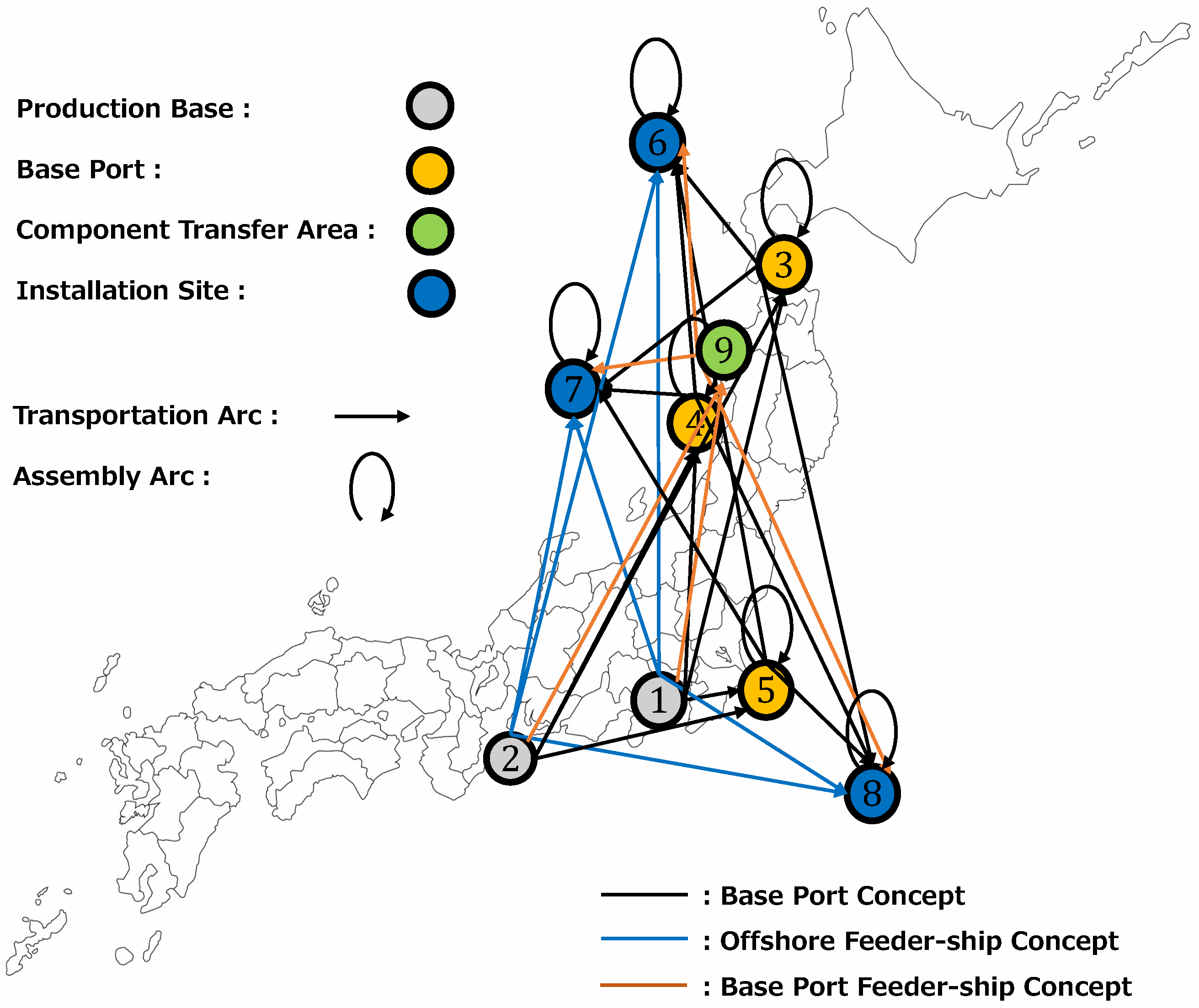
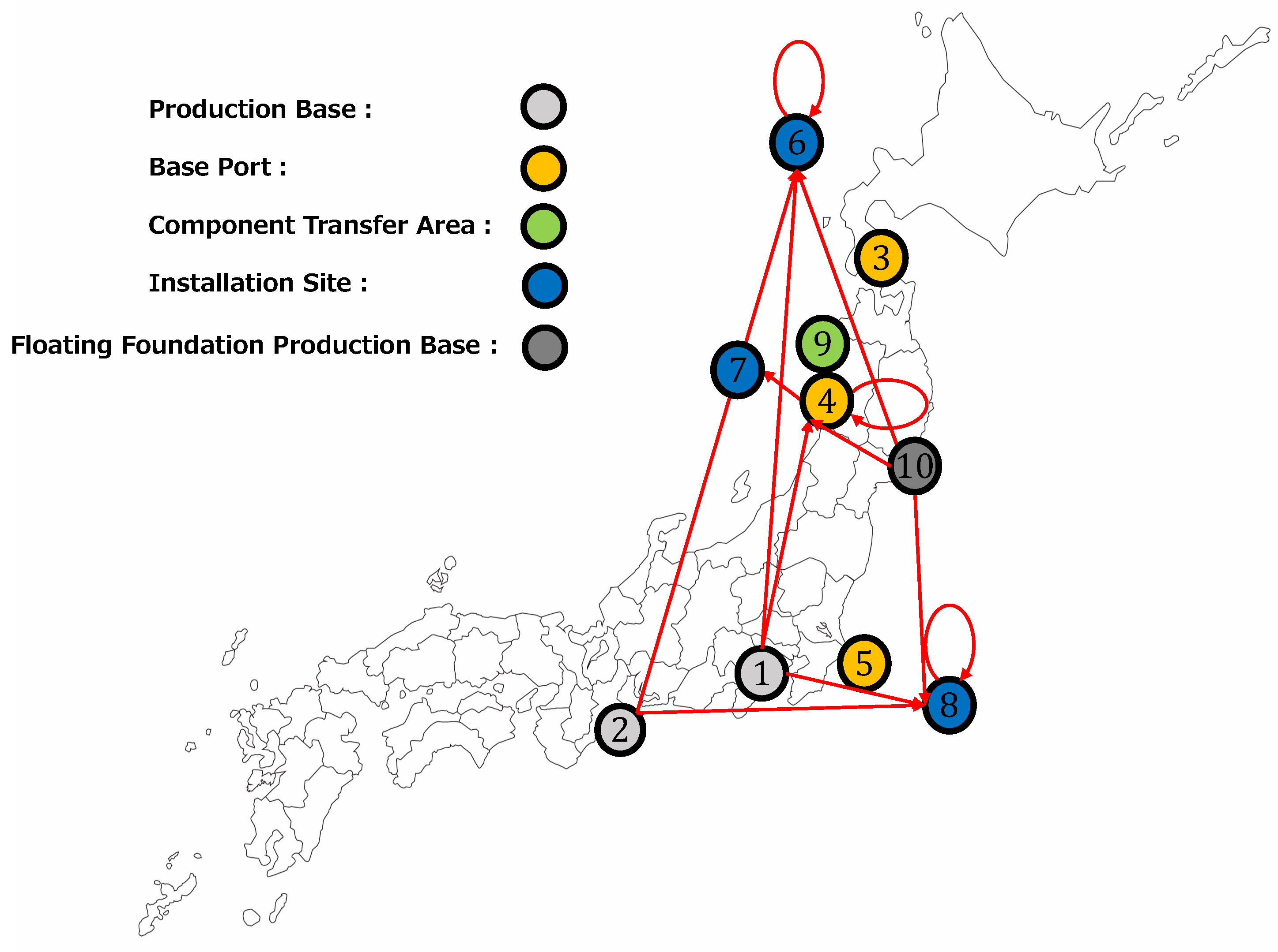
3.1. Case A: Design of Supply Chain Base Plan

3.1.1. Problem Setting

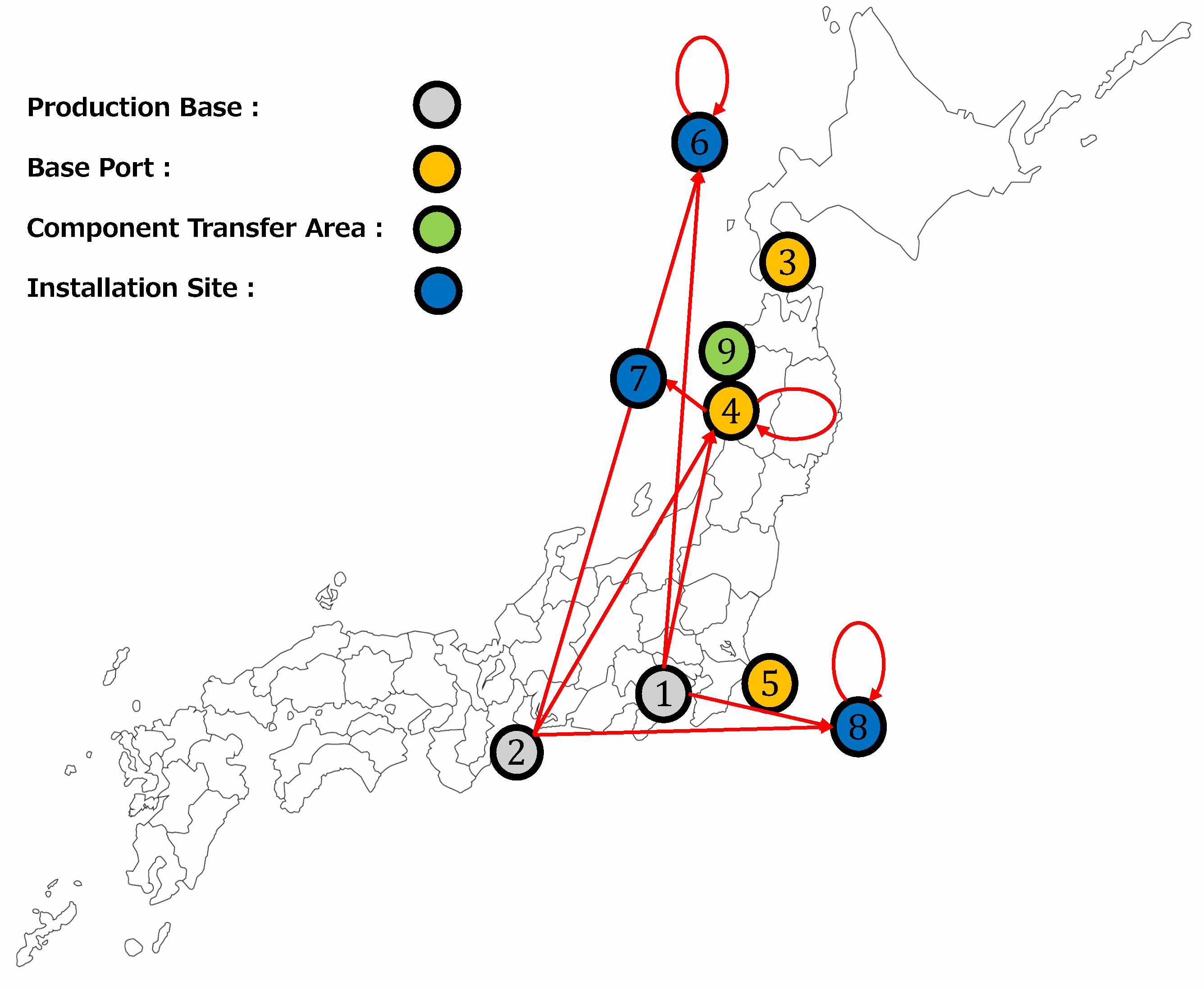
Figure 3 shows the transportation network considering the types of transportation concepts for the production bases, base ports, installation sites, and component transfer area points selected in case A. Equation (16) shows the classification of each arc in this network. In this case study, the assembly arcs are {(3, 3), (4, 4), (5, 5), (6, 6), (7, 7), (8, 7)} and others are transportation arcs.

Equation (17) shows the supply and demand information of each node in the network. The demand was set so that two floating offshore wind turbines would be installed at each of the installation site nodes $\{6,7,8\}$. The supply was set so that each of the production base nodes $\{1,2\}$ would be able to supply components for three floating offshore wind turbines.

Equation (18) shows the transportation capacity of each arc in the network. In Equation (18), it is assumed that the installation vessel can carry two more floating foundations than the transport vessel, and the same number of other components can be transported. Only the installation vessel can transport the completed wind turbine.

Table 1. ${\mathbf{c}}^{a\pm }$ setting.

$\mathit{a}=(\mathit{i},\mathit{j})$		Node j
		1	2	3	4	5	6	7	8	9
Node i	1			29.4	39.0	6.0	47.4	41.4	7.8	40.8
	2			40.8	50.4	15.6	57.0	49.8	14.4	48.0
	3			3.0			32.4	18.0	49.2
	4				3.0		28.8	2.4	69.6
	5					3.0	82.2	68.4	2.4
	6						5.0
	7							5.0
	8								5.0
	9						31.2	6.0	65.4

shows the setup of transportation and assembly costs in each arc. In the proposed method, the cost ${\mathit{c}}^{a_{\pm }}$ of transportation within each arc is expressed as a five-dimensional vector, as shown in Equation (8). But in the case studies in this paper, the total cost for all the components required for a floating offshore wind turbine to be produced at the production base of each component can be shown in Table 1 because of the simple setup of the case studies. Table 1 shows the total cost of one floating offshore wind turbine component or finished product being transported and assembled on each arc. In Table 1, the diagonal areas represent the costs of the assembly arcs, and the other areas represent the costs of the transportation arcs. The absence of a value indicates no transport or assembly arc. The transportation costs for the transportation arcs are set according to the assumed transportation distance by sea between each node. For the arcs assumed to be passed by installation vessels, the transportation costs are calculated by doubling the distance-based value. The costs in the assembly arcs were set so that the cost of conducting assembly operations in the installation site would be higher than that of conducting assembly operations at the base port.

$$a=(i,j)\in \left\{\begin{array}{cc}{\mathcal{A}}_{\mathrm{assembly}}\hfill & \mathrm{if}i=j,\hfill \\ {\mathcal{A}}_{\mathrm{transportation}}\hfill & \mathrm{otherwise}.\hfill \end{array}\right.$$

(16)

$${\mathit{b}}^i=\left\{\begin{array}{cc}{\left(3,9,3,3,0\right)}^{\mathsf{T}}\hfill & \mathrm{if}i\in \{1,2\},\hfill \\ {\left(0,0,0,0,-2\right)}^{\mathsf{T}}\hfill & \mathrm{if}i\in \{6,7,8\},\hfill \\ {\left(0,0,0,0,0\right)}^{\mathsf{T}}\hfill & \mathrm{otherwise}.\hfill \end{array}\right.$$

(17)

$${\mathit{u}}^{a\pm }=\left\{\begin{array}{cc}{\left(3,9,3,3,3\right)}^{\mathsf{T}}\hfill & \mathrm{if}a\in {\mathcal{A}}_{\mathrm{assembly}}\hfill \\ {\left(3,9,3,1,0\right)}^{\mathsf{T}}\hfill & \mathrm{if}a\in {\mathcal{A}}_{\mathrm{transportation}}\hfill \end{array}\right.$$

(18)

3.1.2. Result

A summary of the optimization results obtained with the above problem setup is shown in Figure 4.

Table 2. Detailed optimization results in case A.

$\mathit{a}=(\mathit{i},\mathit{j})$	${\mathit{x}}_{\mathbf{tower}}^{\mathit{a}+},{\mathit{x}}_{\mathbf{tower}}^{\mathit{a}-}$	${\mathit{x}}_{\mathbf{tower}}^{\mathit{a}+},{\mathit{x}}_{\mathbf{tower}}^{\mathit{a}-}$	${\mathit{x}}_{\mathbf{tower}}^{\mathit{a}+},{\mathit{x}}_{\mathbf{tower}}^{\mathit{a}-}$	${\mathit{x}}_{\mathbf{tower}}^{\mathit{a}+},{\mathit{x}}_{\mathbf{tower}}^{\mathit{a}-}$	${\mathit{x}}_{\mathbf{tower}}^{\mathit{a}+},{\mathit{x}}_{\mathbf{tower}}^{\mathit{a}-}$
$(1,4)$	2, 2	6, 6	2, 2	1, 1	0, 0
$(1,6)$	1, 1	3, 3	1, 1	1, 1	0, 0
$(1,8)$	0, 0	0, 0	0, 0	1, 1	0, 0
$(2,4)$	0, 0	0, 0	0, 0	1, 1	0, 0
$(2,6)$	1, 1	3, 3	1, 1	1, 1	0, 0
$(2,8)$	2, 2	6, 6	2, 2	1, 1	0, 0
$(4,4)$	2, 0	6, 0	2, 0	2, 0	0, 2
$(4,7)$	0, 0	0, 0	0, 0	0, 0	2, 2
$(6,6)$	2, 9	6, 0	2, 0	2, 1	0, 2
$(8,8)$	2, 0	6, 0	2, 0	2, 1	0, 2

shows the details of the optimized transport volumes for each arc. The total cost was $242.8$ as a result of the proposed optimization. Figure 4 illustrates that the supply chain for introducing wind turbines was established by integrating two transportation concepts: the base port concept and the offshore feeder-ship concept. Furthermore, the verification confirmed that the supply chain proposed in Table 2 is optimal for the given problem setting and that the proposed method functions effectively.

The optimization results are influenced by the cost settings. In practical applications of the proposed method, not only supply and demand information but also the cost settings for each transportation mode will have a significant impact on the results. Since the unit cost of each transportation mode varies by region, it is crucial to coordinate with relevant stakeholders to establish appropriate cost assumptions when designing the supply chain.

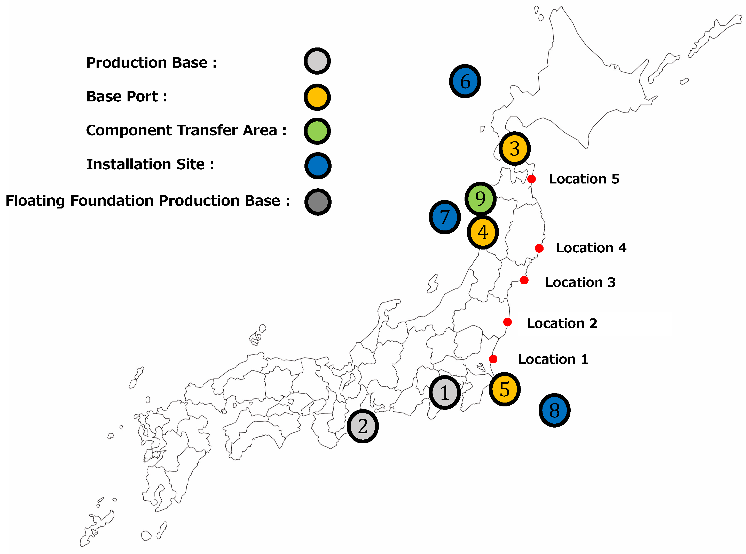
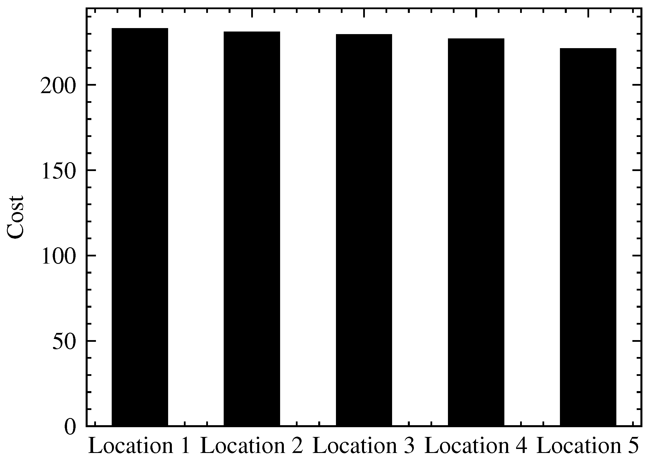
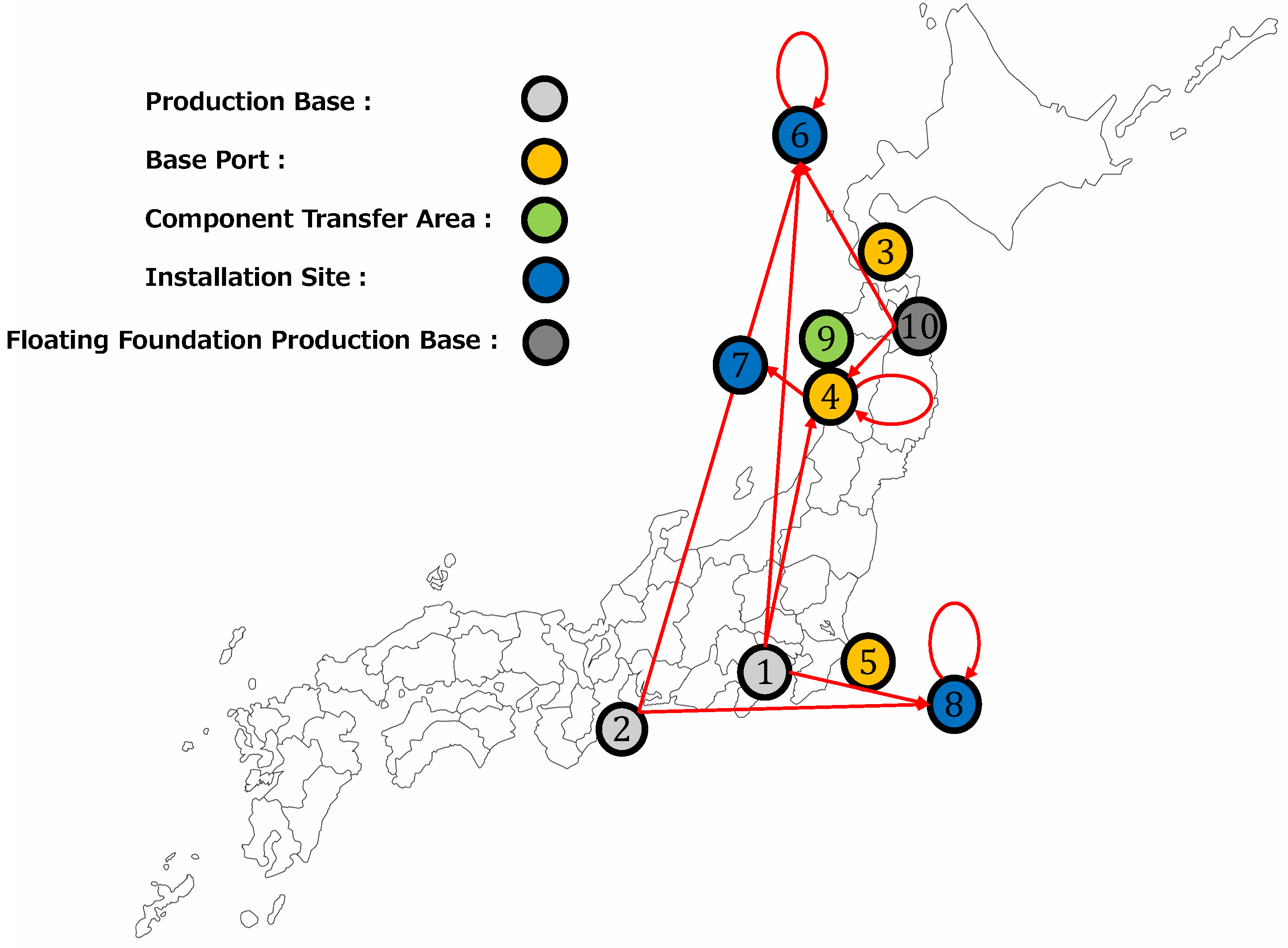
3.2. Case B: Exploring the Optimal Location for Floating Foundation Production Base

3.2.1. Problem Setting

In case B, we assume that a new “floating foundation production base” will be established on the network in case A. For floating offshore wind turbines, not only steel but also concrete are being considered as floating foundation materials. Compared to steel foundations, concrete foundations can be manufactured in any location considering the concrete manufacturing method. The optimal location for the floating foundation production base and supply chain are established using the proposed method.

In this problem, node {10} is the floating foundation production base, which is assumed to be able to produce six units of floating foundations only, which can be transported from node {10} to all other nodes without restriction. Compared to case A, case B has an oversupply of floating foundations. Figure 5 shows the existing nodes in case A and the candidate locations for the floating foundation production base. Optimization calculations are performed using the network shown in Figure 3 plus seven transportation arcs from node $\left\{10\right\}$ to each base port, installation site, and component transfer area.

Table 3. ${\mathbf{c}}^{a\pm }$ setting of each potential location of the floating foundation production base in case B.

$\mathit{a}=(\mathit{i},\mathit{j})$		Node j
		1	2	3	4	5	6	7	8	9
	Location 1			4.3	6.0	0.1	6.9	5.8	0.3	5.6
	Location 2			3.6	5.3	0.7	6.2	5.1	0.7	4.9
	Location 3			2.8	4.5	1.6	5.4	4.3	1.8	4.1
	Location 4			2.0	3.7	2.1	4.7	3.5	2.3	3.3
	Location 5			0.6	2.3	3.7	3.2	2.1	3.4	1.9

shows the costs for the transportation arcs of each potential location of the floating foundation production base in case B. As with the method described in case A, cost values were set based on the distance assumed for transportation between each node by sea. For the arcs that existed in case A, the values in Table 1 were used. As for the transport capacity of the transport arcs, it was assumed that three floating foundations could be transported from node $\left\{10\right\}$ to each arc at a time. The other settings were the same as in case A.

3.2.2. Result

Figure 6 shows the total cost obtained by repeatedly solving the network problem by changing the candidate locations of the floating foundation production base in the case B problem setup. From Figure 6, it can be said that location 5 is the optimal location for the floating foundation production base in case B from the cost point of view.

Figure 7, Figure 8 and Figure 9 summarize the optimization results when a floating foundation production base is located at each potential location. Figure 7, Figure 8, and Figure 9 show the transportation network when the floating foundation production bases are installed at locations 1 and 2 (Figure 7), 3 and 4 (Figure 8), and 5 (Figure 9), respectively.

The only difference between Figure 7 and Figure 8 is the amount of floating foundations transported. In both Figure 7 and Figure 8, components other than the floating foundations are transported from node {2} to node {8}. The difference between Figure 7 and Figure 8 is whether two floating foundations are transported to node {8} from node {10} only, or one each from node {1} and node {10}. From the cost setting, it is cheaper to transport from node {10} to node {8} in Figure 7, while it is cheaper to transport from node {1} to node {8} in Figure 8. However, Equation (18) imposes the constraint that only one foundation can be transported from node {1} to node {8} at most. Therefore, the optimization calculation, using the minimum cost as the objective function, changes the method of transporting the foundation to node {8}.

Similarly, Figure 8 and Figure 9 differ only in the transport of the floating foundation. Compared to Figure 8, in Figure 9, the amount of floating foundations transported to node {8} is changed to one unit each for node {1} and node {2}. In addition, node {1} and node {2} do not transport any component except for floating foundations to node {8}. From the cost setting, when the floating foundation production base reaches location 5, the cost of transporting the floating foundations from node {1} and node {2} to node {8} is cheaper than the cost of transporting the foundations from node {10} to node {8}. As a result, transporting the floating foundations from node {1} and node {2} to node {8} is no longer selected in the proposed method.

From case B, it can be said that the proposed method was able to select the optimal location for the floating foundation production base from among the candidate locations and design the supply chain of introducing wind turbines at that time.

4. Discussion

This paper has dealt with an elementary and small case study of designing a supply chain for introducing floating wind turbines. However, since the proposed method uses linear modeling, optimization calculations can be performed in real time, even when dealing with a large number of supply chain candidates. In addition, the number of floating offshore wind turbines handled can be increased by increasing the number of component types handled by the proposed method.

The design of a specific supply chain for installing floating wind turbines requires a detailed definition of the components of the target floating wind turbine. When targeting the installation of large floating offshore wind turbines or concrete floating foundations, it is assumed that the components will be divided and transported separately. Although not addressed in the case studies in this paper, this case could be handled by changing the value of the transformation matrix B used in the proposed method. In real-world applications, the design of supply chains must consider not only cost minimization, as adopted in this study, but also a broader range of criteria such as environmental impacts [26]. The formulation of objective functions that reflect these multiple dimensions, as well as the investigation of how such formulations influence optimization outcomes, remains an important direction for future research.

Suppose the supply or transportation capacity of the component is insufficient to meet the installation demand of the floating offshore wind turbines. In this case, there is no solution in the constraint equation to solve the problem as a linear programming problem, and optimization cannot be performed in the proposed method. In the proposed method, the amount of supply must be larger than the amount of demand when setting the amount of demand and supply in the design of the network problem. In order to design a long-term deployment plan for floating offshore wind turbines in the future, it will be necessary to examine optimization calculation methods to derive a supply chain for installing floating wind turbines that maximize supply and transportation capacity and to express the portion of demand not met as opportunity loss.

5. Conclusions

This paper developed a method to represent the supply chain of floating offshore wind turbines, including component transportation and wind turbine assembly and installation in a network flow model, and proposed a supply chain design method using the network model. Specifically, the Generalized Multi-Commodity Network Flows (GMCNF) model was applied to the supply chain design problem for installing floating offshore wind turbines to represent the entire process as a network problem. By solving the network model as a linear programming problem, the optimal processes and transportation routes of the supply chain were derived. The case study presents two design scenarios utilizing the model, highlighting the effectiveness of the method. It shows that the model enables the design of a supply chain that incorporates several types of transportation concepts with different locations for assembly and transfer. In addition, it quantitatively evaluates potential new production site locations for floating foundations while considering overall supply chain optimization. By systematically incorporating all conceivable transportation patterns under the GMCNF framework, the proposed approach enables the derivation of an optimal supply chain strategy tailored to floating offshore wind turbine installation.

Future research could explore more complex scenarios and incorporate additional constraints to further enhance the model’s applicability. Increased complexity will necessitate more sophisticated analytical approaches, including the development of mathematical methods to detect structural transition points in the optimal supply chain configuration.

References

1. Bahari, M.; Akbari, Y.; Akbari, N.; Jafari, M.; Qezelbigloo, S.; Zahedi, R.; Yousefi, H. Techno-Economic Analysis and Optimization of a Multiple Green Energy Generation System Using Hybrid Wind, Solar, Ocean and Thermoelectric Energy. Energy Syst. 2024. [Google Scholar] [CrossRef]
2. Kara, O. Assessment of Economic, Energy, and Exergy Efficiencies Using Wind Measurement Mast Data for Different Wind Turbines. Environ. Sci. Pollut. Res. 2023, 30, 97447–97462. [Google Scholar] [CrossRef] [PubMed]
3. Spiru, P.; Simona, P.L. Wind Energy Resource Assessment and Wind Turbine Selection Analysis for Sustainable Energy Production. Sci. Rep. 2024, 14, 10708. [Google Scholar] [CrossRef] [PubMed]
4. Rinne, E.; Holttinen, H.; Kiviluoma, J.; Rissanen, S. Effects of Turbine Technology and Land Use on Wind Power Resource Potential. Nat. Energy 2018, 3, 494–500. [Google Scholar] [CrossRef]
5. Saeed, M.A.; Ahmed, Z.; Zhang, W. Wind energy potential and economic analysis with a comparison of different methods for determining the optimal distribution parameters. Renew. Energy 2020, 161, 1092–1109. [Google Scholar] [CrossRef]
6. Fazelpour, F.; Markarian, E.; Soltani, N. Wind energy potential and economic assessment of four locations in Sistan and Balouchestan province in Iran. Renew. Energy 2017, 109, 646–667. [Google Scholar] [CrossRef]
7. Charabi, Y.; Abdul-Wahab, S. Wind Turbine Performance Analysis for Energy Cost Minimization. Renew. Wind Water Solar 2020, 7, 5. [Google Scholar] [CrossRef]
8. Akbari, N.; Irawan, C.A.; Jones, D.F.; Menachof, D. A Multi-Criteria Port Suitability Assessment for Developments in the Offshore Wind Industry. Renew. Energy 2017, 102, 118–133. [Google Scholar] [CrossRef]
9. Prostean, G.; Badea, A.; Vasar, C.; Octavian, P. Risk Variables in Wind Power Supply Chain. Procedia-Soc. Behav. Sci. 2014, 124, 124–132. [Google Scholar] [CrossRef]
10. Sarker, B.R.; Faiz, T.I. Minimizing Transportation and Installation Costs for Turbines in Offshore Wind Farms. Renew. Energy 2017, 101, 667–679. [Google Scholar] [CrossRef]
11. Kaiser, M.J.; Snyder, B.F. Modeling Offshore Wind Installation Costs on the U.S. Outer Continental Shelf. Renew. Energy 2013, 50, 676–691. [Google Scholar] [CrossRef]
12. Ahn, D.; Shin, S.c.; Kim, S.y.; Kharoufi, H.; Kim, H.c. Comparative Evaluation of Different Offshore Wind Turbine Installation Vessels for Korean West–South Wind Farm. Int. J. Nav. Archit. Ocean. Eng. 2017, 9, 45–54. [Google Scholar] [CrossRef]
13. Vis, I.F.; Ursavas, E. Assessment Approaches to Logistics for Offshore Wind Energy Installation. Sustain. Energy Technol. Assess. 2016, 14, 80–91. [Google Scholar] [CrossRef]
14. Barlow, E.; Tezcaner Öztürk, D.; Revie, M.; Akartunalı, K.; Day, A.H.; Boulougouris, E. A Mixed-Method Optimisation and Simulation Framework for Supporting Logistical Decisions during Offshore Wind Farm Installations. Eur. J. Oper. Res. 2018, 264, 894–906. [Google Scholar] [CrossRef]
15. Faraggiana, E.; Giorgi, G.; Sirigu, M.; Ghigo, A.; Bracco, G.; Mattiazzo, G. A Review of Numerical Modelling and Optimisation of the Floating Support Structure for Offshore Wind Turbines. J. Ocean. Eng. Mar. Energy 2022, 8, 433–456. [Google Scholar] [CrossRef]
16. Maienza, C.; Avossa, A.M.; Picozzi, V.; Ricciardelli, F. Feasibility Analysis for Floating Offshore Wind Energy. Int. J. Life Cycle Assess. 2022, 27, 796–812. [Google Scholar] [CrossRef]
17. Laura, C.S.; Vicente, D.C. Life-cycle cost analysis of floating offshore wind farms. Renew. Energy 2014, 66, 41–48. [Google Scholar] [CrossRef]
18. Myhr, A.; Bjerkseter, C.; Ågotnes, A.; Nygaard, T.A. Levelised cost of energy for offshore floating wind turbines in a life cycle perspective. Renew. Energy 2014, 66, 714–728. [Google Scholar] [CrossRef]
19. Hasumi, T.; Yokoi, T.; Haneda, K.; Chujo, T.; Fujiwara, T. Research on Offshore Installation Time Estimation Model for Floating Offshore Wind Farms. J. Jpn. Soc. Nav. Archit. Ocean. Eng. 2023, 38, 127–139. [Google Scholar] [CrossRef]
20. Poulsen, T.; Lema, R. Is the supply chain ready for the green transformation? The case of offshore wind logistics. Renew. Sustain. Energy Rev. 2017, 73, 758–771. [Google Scholar] [CrossRef]
21. Kruger, T.; Price, S.; Wiedijk, M. Floating Offshore Wind Supply Chain Constraints and Opportunities. In Proceedings of the OTC Offshore Technology Conference, Houston, TX, USA, 6–9 May 2024; p. D021S004R003. Available online: https://onepetro.org/OTCONF/proceedings-pdf/24OTC/2-24OTC/D021S004R003/3403124/otc-35398-ms.pdf (accessed on 1 July 2025.).
22. González, M.O.A.; Nascimento, G.; Jones, D.; Akbari, N.; Santiso, A.; Melo, D.; Vasconcelos, R.; Godeiro, M.; Nogueira, L.; Almeida, M.; et al. Logistic Decisions in the Installation of Offshore Wind Farms: A Conceptual Framework. Energies 2024, 17, 6004. [Google Scholar] [CrossRef]
23. Díaz, H.; Guedes Soares, C. Approach for Installation and Logistics of a Floating Offshore Wind Farm. J. Mar. Sci. Eng. 2023, 11, 53. [Google Scholar] [CrossRef]
24. Ishimatsu, T. Generalized Multi-Commodity Network Flows: Case Studies in Space Logistics and Complex Infrastructure Systems. Doctoral Thesis, Massachusetts Institute of Technology, Cambridge, MA, USA, 2013. [Google Scholar]
25. Ait-Alla, A.; Oelker, S.; Lewandowski, M.; Freitag, M.; Thoben, K.D. A Study of New Installation Concepts of Offshore Wind Farms by Means of Simulation Model. In Proceedings of the Twenty-Seventh (2017) International Ocean and Polar Engineering Conference, San Francisco, CA, USA, 25–30 June 2017; Volume 27, pp. 607–612. [Google Scholar]
26. Bashir, M.B.A. Principle Parameters and Environmental Impacts That Affect the Performance of Wind Turbine: An Overview. Arab. J. Sci. Eng. 2022, 47, 7891–7909. [Google Scholar] [CrossRef] [PubMed]
Figure 1. Overview of proposed method.
Systems 13 00598 g001
Figure 2. Example of supply chain network model.
Systems 13 00598 g002
Figure 3. Overview of the case A problem setting.
Systems 13 00598 g003
Figure 4. Overview of optimization result in case A.
Systems 13 00598 g004
Figure 5. Potential locations of floating foundation production base in case B.
Systems 13 00598 g005
Figure 6. Optimization cost of each potential location.
Systems 13 00598 g006
Figure 7. Overview of the optimization result of locations 1 and 2.
Systems 13 00598 g007
Figure 8. Overview of the optimization result of locations 3 and 4.
Systems 13 00598 g008
Figure 9. Overview of the optimization result of potential site 5.
Systems 13 00598 g009