Hierarchical Modeling and Analysis of an International Conflict Based on Hesitant Fuzzy Linguistic Term Sets

Abstract

In this article, to address the uncertainty of preference information in interrelated conflicts in the real world, a hierarchical conflict modeling and analysis approach based on hesitant fuzzy linguistic term sets (HFLTSs) is proposed. First, considering the hesitancy and fuzziness of decision makers (DMs) when expressing preferences in hierarchical conflicts, a preference representation approach based on HFLTSs is introduced. Building upon hesitant fuzzy linguistic preference, four distinct types of hesitant fuzzy stability definitions of the two-level hierarchical graph model for conflict resolution (HGMCR) are extended, and a corresponding algorithm is developed to solve the global conflict hesitant fuzzy equilibrium states. Finally, this study is applied to investigate the outbreak and development of a specific international conflict, verifying the feasibility and effectiveness of the proposed approach. The hesitant fuzzy equilibrium states of an international conflict indicate that the attitudes of domestic forces reflect a nation’s performance in the warand that the conflict may endure for an extended duration. The hierarchical conflict modeling and analysis approach based on HFLTSs allows DMs to express the hesitation and fuzziness of preferences under uncertainty, facilitates the comprehension of the intrinsic logic behind interactions among DMs at various levels, and enhances the analysis to achieve more foresighted equilibria.

1. Introduction

Conflicts in the real world often consist of small-scale strategic interactions referred to as local conflicts among decision makers (DMs) [1]. These interrelated conflicts are referred to as hierarchical conflicts. Failing to recognize these hierarchical relationships may lead to misjudgments regarding strategic outcomes. For instance, the Russia–Ukraine conflict, the largest international conflict since the Cold War, reflects hierarchical structures through the interactions of national governments at both the national and domestic levels [2]. The Ukrainian government is involved in both a national-level local conflict with Russia and domestic-level local conflicts among various internal forces. To comprehensively explore the outbreak and evolution of the Russia-Ukraine conflict, analysts should not only focus on the national–level conflict between Russia and Ukraine but also investigate the domestic-level roots of the conflicts within both countries.

The hierarchical graph model for conflict resolution (HGMCR), an extension of the classic graph model for conflict resolution (GMCR), has been widely applied to analyze interrelated conflicts with hierarchical structures. The HGMCR introduces local graph models to represent local conflicts and allows for their further decomposition into smaller local conflicts, effectively depicting the complex interactions among multiple DMs at different levels [3]. In the HGMCR, DMs are categorized into common DMs (CDMs) and local DMs (LDMs). CDMs can participate in the decision-making process of all local conflicts, whereas LDMs influence the outcome of only a single local conflict. The HGMCR boasts a flexible theoretical framework that allows for the formulation of new rules based on specific conflict issues, thereby addressing the complexities of real-world conflicts. The Basic HGMCR (BHGMCR), as the foundational model of the HGMCR, consists of two local graphs containing one CDM and two LDMs and has been applied to resolve water diversion conflicts in China [4]. The Duo HGMCR introduces two CDMs, who participate in two related local conflicts, and has been used to analyze market competition between Airbus and Boeing [5]. The General HGMCR includes an arbitrary number of local graphs and has been applied to the greenhouse gas emissions dispute between the USA and China [6]. The two-level and three-level HGMCR embed local graphs at two and three levels, respectively, making them suitable for addressing more complex hierarchical conflicts, such as the aggregate mining conflict in Canada and international climate change negotiations [7,8,9]. Additionally, the introduction of sequential moves, power asymmetry, and coalition analysis has greatly enhanced the practical applicability of the HGMCR [3,10,11].

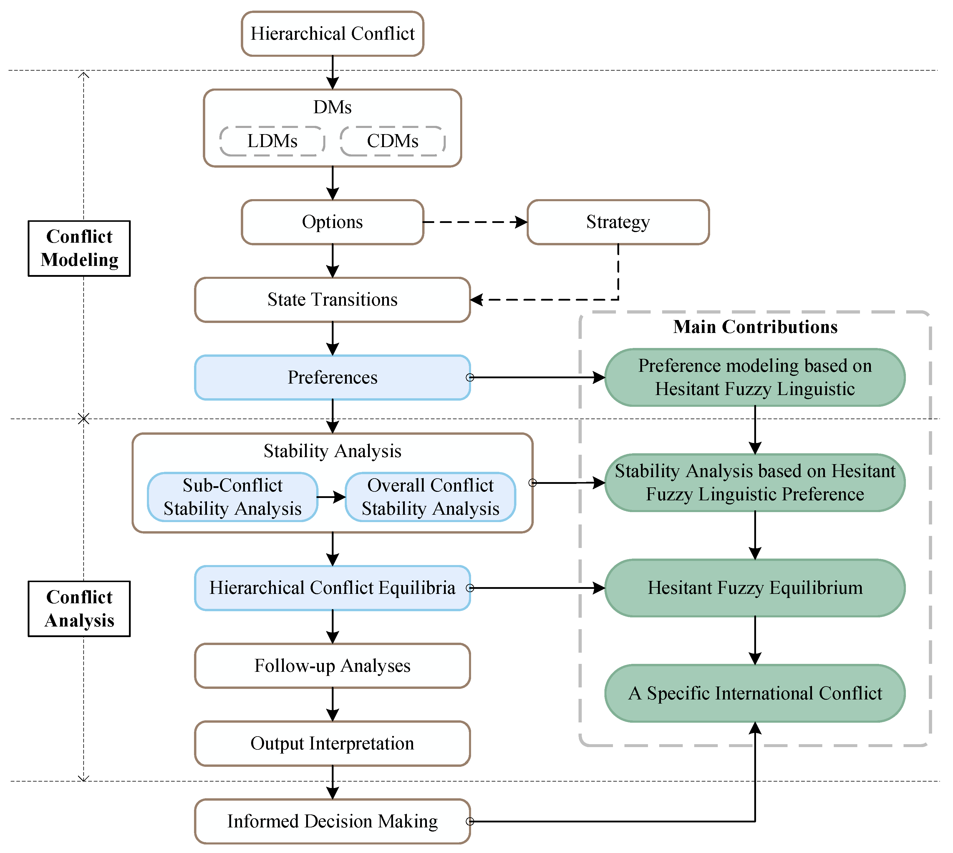
The main process of using the HGMCR to study hierarchical conflicts is illustrated in Figure 1. First, during the conflict modeling phase, it is essential to identify the DMs, options, strategies, state transitions, and preference information. Subsequently, stability analysis and follow-up analyses are conducted to identify stable states and analyze potential equilibrium outcomes and evolutionary processes of the conflict. Among these, preference information is the most critical element in conflict modeling, as it directly impacts the outcomes of the subsequent analysis [12]. In classical GMCR, considering only crisp preference fails to adequately capture the complex and diverse preference information of DMs. Previous studies have expanded the preference structure of the GMCR to include uncertain preference, intensity preference, and hybrid preference [13,14,15]. Additionally, fuzzy preference and gray preference structures have been introduced to the GMCR to better represent the fuzzy characteristics inherent in the decision-making process [16,17]. However, research on the HGMCR remains primarily focused on crisp preference structure and has yet to fully explore how to effectively integrate and analyze the complex preference information of DMs in multi-layered, dynamically changing environments.

Based on the precision of decision-making information, preferences can be classified into deterministic information (such as integers, ordinals, and utility values) and uncertain information (such as rough, fuzzy, and stochastic information) [18]. Hierarchical conflicts in the real world are complex, involving multiple levels of DMs with varying cognitive abilities, behavioral traits, and decision-making styles, making accurate characterization challenging. As a result, preference information from DMs is often indeterminate and uncertain, making it challenging to precisely express their preferences for feasible states. To capture the uncertain preference information of DMs, existing studies have proposed fuzzy preference relations, wherein the preference of each DM is represented as fuzzy information [19]. However, in real-world conflicts, DMs often prefer to evaluate choices using natural language terms or phrases rather than numerical values [20]. This approach is known as the fuzzy linguistic approach. Since fuzzy linguistic information aligns more closely with human cognitive processes, fuzzy linguistic preferences have been widely applied and developed in fields such as personnel evaluation and information retrieval [21,22]. Fuzzy linguistic preferences qualitatively represent DMs’ suggestion or preferences through linguistic variables, such as “poor reliability”, “average quality”, and “excellent performance”. Considering the time constraints, knowledge limitations, and incomplete information that DMs face during in-depth analysis, a single linguistic term is often insufficient to fully capture their preference information. To address this, hesitant fuzzy linguistic term sets (HFLTSs) allow DMs to expand their range of expression from a single linguistic term to a linguistic term interval, such as “between easy and very easy”. HFLTSs have been extensively applied in fields such as undergraduate teaching auditing and evaluation, financial performance evaluation, and air pollution early warning systems [23,24,25]. They effectively simulate real-world decision-making processes, particularly in complex hierarchical conflicts, where DMs’ preferences are hesitant and fuzzy, making the decision-making process more reflective of actual situations.

To address the challenge of preference uncertainty among DMs at different levels within hierarchical conflicts, this paper introduces HFLTSs into the HGMCR framework. The main contributions of this paper within the HGMCR framework are illustrated in Figure 1. First, this paper integrates HFLTSs into hierarchical conflict preference modeling, addressing the representation problem of hesitant fuzzy preferences among DMs in the two-level HGMCR. Then, the paper extends and defines four types of hesitant fuzzy stability in the Two-level HGMCR and, based on this, develops an algorithm for solving the global conflict hesitant fuzzy equilibrium states in the two-level HGMCR. Finally, this study applies the proposed approach to explore the outbreak and development of a specific international conflict, validating the effectiveness of the two-level HGMCR modeling and analysis approach based on HFLTSs. The hesitant fuzzy equilibrium states of an international conflict indicate that the attitudes of domestic forces reflect a nation’s performance in the war and that the conflict may endure for an extended duration.

The remainder of this paper is organized as follows. Section 2 provides a brief introduction to the BHGMCR and HFLTSs. Section 3 presents the two-level HGMCR preference modeling approach based on HFLTSs and defines four types of hesitant fuzzy stability definitions. Section 4 develops algorithms for calculating equilibrium in the two-level HGMCR Section 5 describes the application of the proposed approach in a case study involving a specific international conflict. Finally, Section 6 provides the conclusions of the work.

2. Preliminaries

2.1. BHGMCR

The classical GMCR supposes that all DMs are engaged in a singular, unified conflict. However, in an HGMCR consisting of multiple local graph models, distinct DMs participate in separate local conflicts. Specifically, LDMs can only move within their own local conflicts, while CDMs can move across all local conflicts. For example, a BHGMCR (G) consists of two local graph models ($G^{\left(1\right)}$ and $G^{\left(2\right)}$), along with one CDM (C) and two LDMs ($l_1$ and $l_2$). In the BHGMCR, C is shared between $G^{\left(1\right)}$ and $G^{\left(2\right)}$, while $l_1$ and $l_2$ are restricted to $G^{\left(1\right)}$ and $G^{\left(2\right)}$, respectively. The formal definition of the BHGMCR is paraphrased below.

Definition 1 

((BHGMCR) [4]). Assume that two conflicts can be represented by two quadruples:

$$G^{\left(1\right)}=〈\left\{C,l_1\right\},S^{\left(1\right)},A^{\left(1\right)},{\succsim }^{\left(1\right)}〉$$

(1)

and

$$G^{\left(2\right)}=〈\left\{C,l_2\right\},S^{\left(2\right)},A^{\left(2\right)},{\succsim }^{\left(2\right)}〉.$$

(2)

The graph model (G), composed of the local graph models ($G^{\left(1\right)}$ and $G^{\left(2\right)}$), is referred to as the BHGMCR, where

• $N=\left\{C,l_1,l_2\right\}$ represents the set of DMs in all local conflicts;
• $S=S^{\left(1\right)}\times S^{\left(2\right)}$ represents the state set (S) of the hierarchical graph (G) as the Cartesian product of the states of the two local graphs;
• $A=A^{\left(1\right)}\cup A^{\left(2\right)}$ denotes the action set (A) in the hierarchical graph (G) as the union of the action sets of the two local graphs;
• $\succsim \supseteq {\succsim }^{\left(1\right)}\cup {\succsim }^{\left(2\right)}$ indicates that the preference relations in the hierarchical graph (G) are partially derived from the preference relations in the two local graphs. The preference relations include five types: more preferred (≻ ), less preferred (≺), indifferent (∽), not worse than (≿), and not better than (≾). The preference relations of each DM over the state set (S) is complete, transitive, and reflexive.

Suppose that a BHGMCR (G) consists of two local graphs ($G^{\left(1\right)}$ and $G^{\left(2\right)}$). $G^{\left(1\right)}$ is considered to be more important than, less important than, or equally important as $G^{\left(2\right)}$, denoted as $G^{\left(1\right)}>G^{\left(2\right)}$, $G^{\left(1\right)}<G^{\left(2\right)}$, and $G^{\left(1\right)}\sim G^{\left(2\right)}$, respectively.

The options represent the strategic choices made by the DMs in the conflict. Each DM has at least one option. Each option can be either selected, denoted as “Y”, or not selected, denoted as “N”. Let the set of options in the HGMCR be denoted as $O=\left\{o_1,\dots ,o_m\right\}$, where $o_j\in O$ for $j=1,\dots ,m$. The selection of option $o_j$ (whether “Y” or “N”) is defined as a function of $o_j$, denoted as $f\left(o_j\right)$. The DM’s choice of option $o_j$ is represented by $f\left(o_j\right)$ for $j=1,\dots ,m$:

$$f\left(o_j\right)=\left\{\begin{array}{c}Y,o_j\mathrm{is}\mathrm{taken}\hfill \\ N,o_j\mathrm{is}\mathrm{not}\mathrm{taken}.\hfill \end{array}\right.$$

(3)

The outcome of the conflict (referred to as the state in the HGMCR) is the combination of all selected options. For example, in BHGMCR G, the set of options is given by $O=\left\{o_1,o_2,o_3\right\}$. For a state ($s\in S$), the choices for all options are represented as $f\left(o_1\right)=Y$, $f\left(o_2\right)=N$, and $f\left(o_3\right)=Y$. Therefore, for state s, options $o_1$, $o_2$, and $o_3$ are selected as Y, N, and Y, respectively, which can be represented as $s=\left(YNY\right)$.

2.2. HFLTSs

The HFLTSs enable DMs to evaluate alternatives using one or more linguistic terms, thereby addressing situations of indecision during the decision-making process. The mathematical representation of the HFLTSs is provided below.

Definition 2 

((HFLTS) [26]). Let X be a fixed set, and let $T=\left\{t_{\alpha }|\alpha =-\tau ,\dots ,-1,0,1,\dots ,\tau \right\}$ denote a symmetric-index linguistic term set, where the lower and upper bounds of the linguistic terms are $t_{-\tau }$ and $t_{\tau }$, respectively. HFLTS $H_T$ on X is a finite subset of continuous linguistic terms from T, which can be represented as

$$H_T=\left\{〈x_i,h_T\left(x_i\right)〉|x_i\in X\right\},$$

(4)

where $h_T\left(x_i\right)$ is referred to as the hesitant fuzzy linguistic element (HFLE), which represents the degree of affiliation of the linguistic variable (i.e., decision alternative) ($x_i$) in the linguistic term set (T). Specifically, $h_T\left(x_i\right)$ is a set of linguistic terms from T, denoted as $h_T\left(x_i\right)=\left\{t_{{\varphi }_l}|t_{{\varphi }_l}\left(x_i\right)\in T,l=1,2,\dots ,L\right\}$, where L represents the number of linguistic terms in $h_T\left(x_i\right)$.

In real-world decision-making processes involving conflicts, DMs commonly utilize linguistic expressions to represent cognitive judgments that are clear and applicable, such as “between slightly better and strongly better” and “at least significantly better”. However, such direct linguistic expressions are insufficient to support subsequent computational analysis. Therefore, it is necessary to use a transformation function ($E_{G_H}$) based on a context-free grammar to convert linguistic expressions into an HFLE. The mathematical representation of the transformation function ($E_{G_H}$) is expressed as follows [27].

$$\left\{\begin{array}{c}{E}_{G_H}\left(t_{\alpha }\right)=\left\{t_{\alpha }|t_{\alpha }\in T\right\};\hfill \\ E_{G_H}\left(\mathrm{at}\mathrm{most}{t}_{\beta }\right)=\left\{t_{\alpha }|t_{\alpha }\in T\mathrm{and}{t}_{\alpha }\le t_{\beta }\right\};\hfill \\ E_{G_H}\left(\mathrm{lower}\mathrm{than}{t}_{\beta }\right)=\left\{t_{\alpha }|t_{\alpha }\in T\mathrm{and}{t}_{\alpha }<t_{\beta }\right\};\hfill \\ E_{G_H}\left(\mathrm{at}\mathrm{least}{t}_{\beta }\right)=\left\{t_{\alpha }|t_{\alpha }\in T\mathrm{and}{t}_{\alpha }\ge t_{\beta }\right\};\hfill \\ E_{G_H}\left(\mathrm{great}\mathrm{than}{t}_{\beta }\right)=\left\{t_{\alpha }|t_{\alpha }\in T\mathrm{and}{t}_{\alpha }>t_{\beta }\right\};\hfill \\ E_{G_H}\left(\mathrm{between}{t}_{\beta }\mathrm{and}{t}_{{\beta }^{\prime }}\right)=\left\{t_{\alpha }|t_{\alpha }\in T\mathrm{and}{t}_{\beta }\le t_{\alpha }\le t_{{\beta }^{\prime }}\right\}.\hfill \end{array}\right.$$

(5)

Assume that a DM is tasked with evaluating the potential effects of three strategies, denoted as $x_1$, $x_2$, and $x_3$. The objective of the decision-making process is to assess the effectiveness of these strategies. The HFLTS used for this evaluation is defined as follows: $T=\{t_{-3}=\mathrm{strongly}\mathrm{inferior},t_{-2}=\mathrm{inferior},t_{-1}=\mathrm{slightly}\mathrm{inferior}$, $t_0=\mathrm{indifferent},t_1=\mathrm{slightly}\mathrm{superior},t_2=\mathrm{superior},t_3=\mathrm{strongly}\mathrm{superior}\}$.

It is obvious that providing complex cognitive judgments of HFLTS is a more natural and direct approach for DMs. Suppose the DM evaluates the effectiveness of three strategies using HFLTS T, assigning qualitative expressions such as “at least superior”, “slightly superior”, and “between indifferent and superior” to the strategies. Based on the transformation function ($E_{G_H}$), these three qualitative evaluations can be converted into the following HFLTS: $H_T\left(x\right)=\left\{〈x_1,h_T\left(x_1\right)〉,〈x_2,h_T\left(x_2\right)〉,〈x_3,h_T\left(x_3\right)〉\right\}$, where $h_T\left(x_1\right)=\left\{t_2,t_3\right\}$, $h_T\left(x_2\right)=\left\{t_1\right\}$, and $h_T\left(x_3\right)=\left\{t_0,t_1,t_2\right\}$ represent three HFLEs.

3. Two-Level HGMCR Based on HFLTS

3.1. Two-Level HGMCR

The Two-level HGMCR consists of two BHGMCRs, as shown in Figure 2. At the top level, a local conflict is formed between two CDMs ($d_1^1$ and $d_2^1$). The formal definition of the two-level HGMCR is formally given in the following [8].

Definition 3 

(Two-level HGMCR). Let two BHGMCRs be represented as

$$G_1^2=〈\left\{d_1^1,d_{11}^2,d_{12}^2\right\},S_1^2,A_1^2,{\succsim }_1^2〉$$

(6)

and

$$G_2^2=〈\left\{d_2^1,d_{21}^2,d_{22}^2\right\},S_2^2,A_2^2,{\succsim }_2^2〉.$$

(7)

At the top level, the local graph model containing the two CDMs ($i_1^1$ and $i_2^1$) is denoted as

$$G_0^1=〈\left\{d_1^1,d_2^1\right\},S_0^1,A_0^1,{\succsim }_0^1〉,$$

(8)

where $O_0^1\bigcap O_1^2\bigcap O_2^2=⌀$. Then, a two-level HGMCR is defined as

$$G^H=G_0^1\bigcup G_1^2\bigcup G_2^2=〈N^H,S^H,A^H,{\succsim }^H〉.$$

(9)

where $N^H=\left\{d_1^1,d_2^1,d_{11}^2,d_{12}^2,d_{21}^2,d_{22}^2\right\}$ and $S^H\subset S_0^1\times S_1^2\times S_2^2$.

In $G^H$, state set $S^H$ is a subset of the Cartesian product of $S_0^1$, $S_1^2$, and $S_2^2$. A state ($s^H\in S^H$) can be represented as $s^H=\left(s_0^1,s_1^2,s_2^2\right)$, where $s_0^1\in S_0^1$, $s_1^2\in S_1^2$, and $s_2^2\in S_2^2$.

The preferences of DMs in $G^H$ can be determined as follows:

For $d_1^1$ taking part in $G_0^1$ and $G_1^2$, if $G_0^1>G_1^2$, two states ($s^H,t^H\in S^H$, where $s^H=\left(s_0^1,s_1^2,s_2^2\right)$ and $t^H=\left(t_0^1,t_1^2,t_2^2\right)$) can be compared as follows:

• $s^H\succ t^H$, if $s_0^1\succ t_0^1$;
• $s^H\succ t^H$, if $s_0^1\sim t_0^1$ and $s_1^2\succ t_1^2$.

For LDMs, preferences in $G^H$ are determined analogously to those in the BHGMCR. For example, $s^H=\left(s_0^1,s_1^2,s_2^2\right)$ and $t^H=\left(t_0^1,t_1^2,t_2^2\right)$ can be compared for $d_{11}^2$ as $s^H\succ t^H$ if $s_1^2\succ t_1^2$.

3.2. Hesitant Fuzzy Linguistic Preference

To capture the hesitant fuzzy linguistic preferences of each DM in hierarchical conflicts, this section defines the hesitant fuzzy linguistic preference relation (HFLPR) for each state in the two-level HGMCR based on HFLTSs. When conducting pairwise comparisons of different states in hierarchical conflicts, DMs utilize HFLPRs to express preferences. This approach effectively aligns with human cognitive processes, particularly in uncertain situations, as it facilitates intuitive preference articulation while offering flexibility in handling ambiguous judgments.

Definition 4 

(HFLPR). Let $S^H=\left\{s_1^H,s_2^H,\dots ,s_m^H\right\}$ denote the state set in the two-level HGMCR ($G^H$) and $T=\left\{t_{\alpha }|\alpha =-\tau ,\dots ,-1,0,1,\dots ,\tau \right\}$ represent the linguistic term set. The HFLPR for the states in $S^H$ is an $m\times m$ matrix, denoted as $H={\left\{h^{ij}\right\}}_{m\times m}$.

Specifically, $h^{ij}=\left\{h^{ij\left(l\right)}|l=1,2,\dots ,L\right\}\left(h^{ij\left(l\right)}\in T\right)$ represents the HFLE, which indicates the preference relation between state $s_i^H$ and state $s_j^H$. The L linguistic terms in $h^{ij}$ are arranged in ascending order.

To facilitate subsequent stability analysis, it is necessary to convert the HFLPR of each DM regarding the states in the hierarchical conflicts into numerical values. Therefore, this paper introduces semantic scale functions that map each linguistic term to the interval of $\left[-1,1\right]$, thereby assigning appropriate semantic values to the linguistic terms.

Let $T=\left\{t_{\alpha }|\alpha =-\tau ,\dots ,-1,0,1,\dots ,\tau \right\}$ represent the linguistic term set, and let ${\theta }_{\alpha }$ denote the semantics of $t_{\alpha }$. The linguistic terms can be mapped to their corresponding semantics through a linguistic scale function, i.e., $f:t_{\alpha }\to {\theta }_{\alpha }$, where f is strictly monotonically increasing and satisfies $f\left(\alpha \right)\in \left[0,1\right]$. 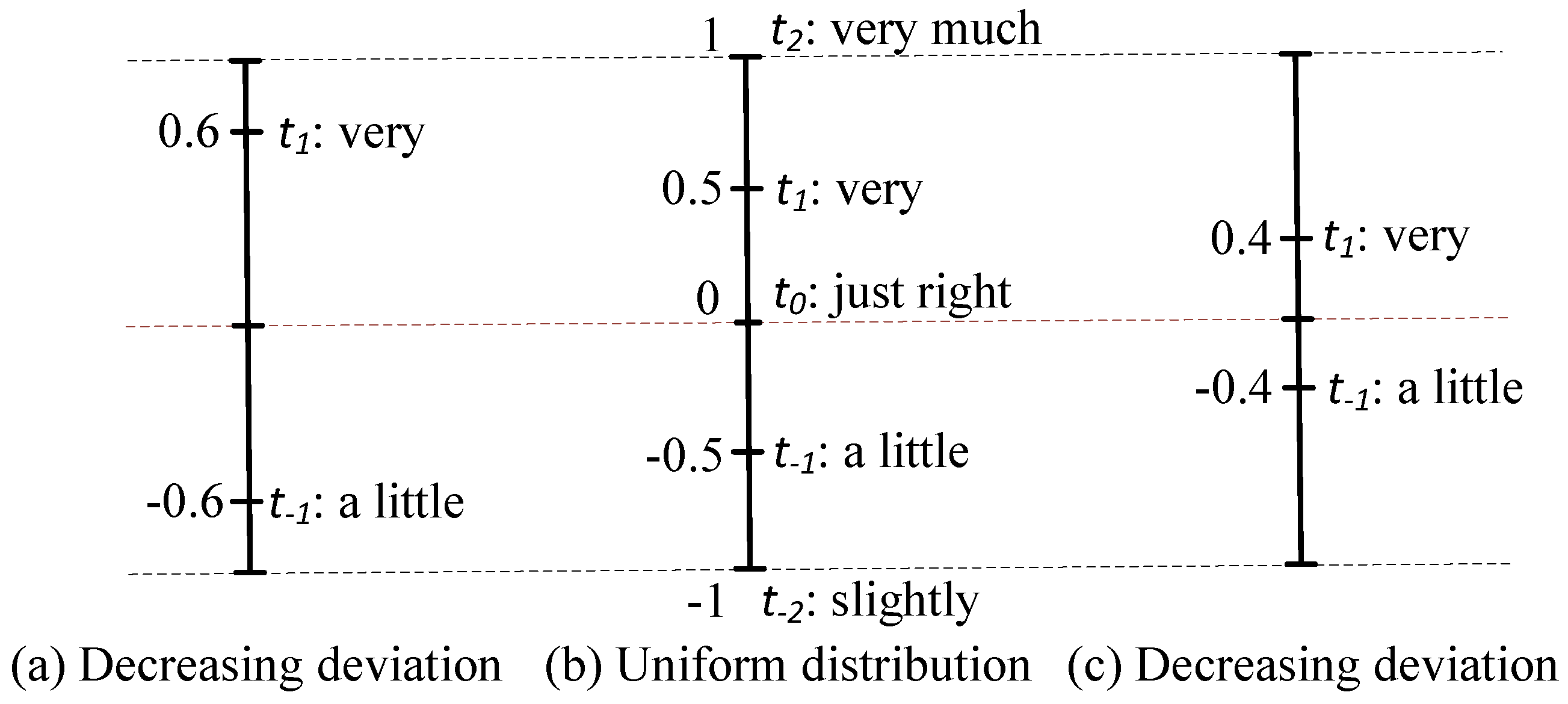Based on the distribution of semantics, the linguistic scale function can be classified into three types: a decreasing deviation distribution, uniform distribution, and increasing deviation distribution. A brief introduction to each function is provided below [28].

1.

Decreasing deviation. Starting from $t_0$, the deviation between two adjacent linguistic terms decreases:

$$f\left(t_{\alpha }\right)=\left\{\begin{array}{c}{\displaystyle \frac{{\tau }^{\zeta }-{\left(-\alpha \right)}^{\zeta }}{2{\tau }^{\zeta }}},\mathrm{if}\alpha =-\tau ,\dots ,0\hfill \\ {\displaystyle \frac{{\tau }^{\zeta }+{\alpha }^{\zeta }}{2{\tau }^{\zeta }}},\mathrm{if}\alpha =0,\dots ,\tau \hfill \end{array}\right.$$

(10)

where $\zeta ,\xi \in \left(0,1\right]$ represent the risk attitudes toward “negative” and “positive” outcomes, respectively. Optimistic individuals tend to prefer larger values of $\zeta$ and $\xi$, whereas smaller values are more appropriate for conservative individuals.

2.

Uniform distribution.

$$f\left(t_{\alpha }\right)={\displaystyle \frac{\alpha +\tau }{2\tau }}.$$

(11)

3.

Increasing deviation. Starting from $t_0$, the deviation between two adjacent linguistic terms increases:

$$f\left(t_a\right)=\left\{\begin{array}{c}{\displaystyle \frac{{\phi }^{\tau }-{\phi }^{-\alpha }}{2{\phi }^{\tau }-2}},\mathrm{if}\alpha =-\tau ,\dots ,0\hfill \\ {\displaystyle \frac{{\phi }^{\tau }+{\phi }^{\alpha }-2}{2{\phi }^{\tau }-2}},\mathrm{if}\alpha =0,\dots ,\tau \hfill \end{array}\right.$$

(12)

where $\phi$ is directly proportional to the degree of deviation and varies depending on the specific problem. It must be greater than 1 to ensure that $f\left(t_a\right)$ is monotonically increasing.

Figure 3 vividly illustrates three types of semantic distributions for the linguistic term sets. Based on the linguistic scale function, the HFLPR can be converted into numerical values.

Definition 5 

(Semantic value). Let $T=\left\{t_{\alpha }|\alpha =-\tau ,\dots ,-1,0,1,\dots ,\tau \right\}$ represent the linguistic term set. For states $s_i^H,s_j^H\in S^H$, the semantic values of the HFLE ($h^{ij}=\left\{h^{ij\left(l\right)}|l=1,2,\dots ,L\right\}$), denoted as $SV\left(h^{ij}\right)$, can be defined as follows:

$$SV\left(h^{ij}\right)=\left[f\left(h^{ij\left(1\right)}\right),f\left(h^{ij\left(2\right)}\right),\dots ,f\left(h^{ij\left(L\right)}\right)\right],$$

(13)

where $h^{ij\left(l\right)}\in T$ and $f\left(h^{ij\left(l\right)}\right)$ represents the semantic value of the linguistic term ($h^{ij\left(l\right)}$). This value can be computed based on the DM’s psychological characteristics using Equation (10), (11), or (12).

The semantic score of the HFLE ($h^{ij}$) can then be calculated using the following formula:

$$f\left(h^{ij}\right)=\sum _{l=1}^{L}f\left(h^{ij\left(l\right)}\right)/L.$$

(14)

Therefore, for DM $d\in N^H$ and states $s_i^H,s_j^H\in S^H$, the preference of DM d, denoted as $P_d$, can be determined by calculating the semantic scores of the corresponding hesitant fuzzy preference matrix ($H_d$):

$$P_d={\left\{f\left(h_d^{ij}\right)\right\}}_{m\times m},$$

(15)

where $f\left(h_d^{ij}\right)$ represents the semantic score of the HFLPR of DM d regarding state $s_i^H$ relative to $s_j^H$.

3.3. Hesitant Fuzzy Stability Definition

In strategic conflicts, DMs must decide whether to maintain the current state or transition to a more favorable one. Different DMs may evaluate the optimal choice from a given state according to their individual criteria. In other words, each DM in the conflict may decide whether to transition to an accessible state based on a threshold of the hesitant fuzzy relative strength of preference (HFRSP).

Definition 6 

(HFRSP). For DM $d\in N^H$ and states $s^H,t^H\in S^H$, the HFRSP regarding state $s^H$ relative to state $t^H$ is defined as follows:

$${\alpha }_d\left(s^H,t^H\right)=f\left(h_d^{st}\right)-f\left(h_d^{ts}\right)=P_d\left(s^H,t^H\right)-P_d\left(t^H,s^H\right).$$

(16)

Note that for DM $d\in N^H$ and states $s^H,t^H\in S^H$, it holds that $-1\le {\alpha }_d\left(s^H,t^H\right)\le 1$. Specifically,

• ${\alpha }_d\left(s^H,t^H\right)=-{\alpha }_d\left(t^H,s^H\right)$;
• ${\alpha }_d\left(s^H,t^H\right)=1$ indicates that for DM d, state $s^H$ is strictly preferred over state $t^H$;
• ${\alpha }_d\left(s^H,t^H\right)=0$ indicates that DM d considers state $s^H$ and state $t^H$ to be indifferent;
• ${\alpha }_d\left(s^H,t^H\right)=-1$ indicates that DM d considers state $t^H$ to be strictly preferred over state $s^H$.

The threshold of the HFRSP is referred to as the hesitant fuzzy satisfyingthreshold (HFST). For DM $d\in N^H$, the HFST of DM d is denoted as ${\gamma }_d$.

Definition 7 

(HFUI). A state ($t^H$) is a hesitant fuzzy unilateral improvement (HFUI) for DM d from state $s^H$ if and only if the HFRSP of DM d with respect to states $s^H$ and $t^H$ exceeds d’s HFST, i.e., ${\alpha }_d\left(t^H,s^H\right)\ge {\gamma }_d$. The list of HFUIs for DM d starting from state $s^H$ can be expressed as follows:

$$R_{d,{\gamma }_d}^{+}\left(s^H\right)=\left\{t^H\in R_d\left(s^H\right)|{\alpha }_d\left(t^H,s^H\right)\ge {\gamma }_d\right\},$$

(17)

where $R_d\left(s^H\right)$ denotes the reachable list for DM d from state $s^H$.

Stability definitions characterize the behavior patterns of DMs and suggest strategic resolutions. Within the GMCR framework, four major stability definitions are studied: Nash stability [29], General Meta-Rationality (GMR) stability [30], Symmetric Meta-Rationality (SMR) stability [30], and Sequential (SEQ) stability [31]. Based on the HFLPR, the corresponding stability definitions for the two-level HGMCR are defined, including Hierarchical Hesitant Fuzzy Nash (HHFNash) stability, Hierarchical Hesitant Fuzzy GMR (HHFGMR) stability, Hierarchical Hesitant Fuzzy SMR (HHFSMR) stability, and Hierarchical Hesitant Fuzzy SEQ (HHFSEQ) stability.

In the two-level HGMCR ($G^H$), for DM $d\in N^H$, states $s^H,t^H,u^H,v^H\in S^H$ assume that the other DMs in $N^H$, except d, form an opponents’ alliance ($N^H\setminus \left\{d\right\}$).

Definition 8 

(HHFNash). A state ($s^H\in S^H$) is HHFNash stable for DM $d\in N^H$, denoted as $s^H\in S_d^{HHFNash}$, if and only if $R_{d,{\gamma }_d}^{+}\left(s^H\right)=⌀$.

Definition 9 

(HHFGMR). A state ($s^H\in S^H$) is HHFGMR stable for DM $d\in N^H$, denoted as $s^H\in S_d^{HHFGMR}$, if and only if, for any $t^H\in R_{d,{\gamma }_d}^{+}\left(s^H\right)$, there exists at least one $u^H\in R_{N\setminus \left\{d\right\},{\gamma }_{N\setminus \left\{d\right\}}}\left(t^H\right)$ such that ${\alpha }_d\left(u^H,s^H\right)<{\gamma }_d$.

Definition 10 

(HHFSMR). A state ($s^H\in S^H$) is HHFSMR stable for DM $d\in N^H$, denoted as $s^H\in S_d^{HHFSMR}$, if and only if, for any $t^H\in R_{d,{\gamma }_d}^{+}\left(s^H\right)$, there exists at least one $u^H\in R_{N\setminus \left\{d\right\}}\left(t^H\right)$ such that ${\alpha }_d\left(u^H,s^H\right)<{\gamma }_d$ and, for all $v^H\in R_d\left(u^H\right)$, ${\alpha }_d\left(v^H,s^H\right)<{\gamma }_d$.

Definition 11 

(HHFSEQ). A state ($s^H\in S^H$) is HHFSEQ stable for DM $d\in N^H$, denoted as $s^H\in S_d^{HHFSEQ}$, if and only if, for any $t^H\in R_{d,{\gamma }_d}^{+}\left(s^H\right)$, there exists at least one $u^H\in R_{N\setminus \left\{d\right\},{\gamma }_{N\setminus \left\{d\right\}}}^{+}\left(t^H\right)$ such that ${\alpha }_d\left(u^H,s^H\right)<{\gamma }_d$.

In each local graph, a state ($s^H\in S^H$) is considered a local hierarchical hesitant fuzzy equilibrium under the given hierarchical hesitant fuzzy stability definition if and only if $s^H$ is hierarchical hesitant fuzzy stable for all DMs in the corresponding local graph. In the hierarchical graph ($G^H$), a state ($s^H\in S^H$) is considered a global hierarchical hesitant fuzzy equilibrium under the given hierarchical hesitant fuzzy stability definition if and only if $s^H$ is hierarchical hesitant fuzzy stable for all DMs in $G^H$.

4. Algorithms for Calculating Equilibrium in the Two-Level HGMCR

4.1. Hesitant Fuzzy Stabilities in the Two-Level HGMCR

To calculate the global hesitant fuzzy stabilities and equilibrium states of the two-level HGMCR, the interrelationships between hesitant fuzzy stabilities in the hierarchical graph and those in the local graphs are investigated based on the theorems that relate local stability to global stability in the two-level HGMCR [8].

In the two-level HGMCR, assume that a DM only considers countermoves from adjacent DMs—for instance, in a specific international conflict ($G^H$) between Country A ($d_1^1$) and Country B ($d_2^1$). $d_1^1$ focuses on the actions of other DMs at the national level ($d_2^1$) and the different forces within its own country ($d_{11}^2$ and $d_{12}^2$), while the DMs of $d_2^1$’s internal forces have a limited impact on $d_1^1$. Similarly, the different forces within $d_1^1$ are not concerned with the actions of internal forces in $d_2^1$ but are primarily focused on the decisions made by $d_1^1$.

Therefore, adjacency for representative DMs in $G^H$ is assumed as follows:

• $d_1^1$: adjacent to $d_{11}^2$, $d_{12}^2$, and $d_2^1$;
• $d_{11}^2$: adjacent to $d_{12}^2$ and $d_1^1$.

Based on this assumption and the theorems that relate local stability to global stability in the two-level HGMCR, theorems are presented to describe the interrelationships between hesitant fuzzy stabilities in the hierarchical graph and those in the local graphs.

Theorem 1 

(HHFNash for ${\mathit{d}}_{\mathbf{1}}^{\mathbf{1}}$). Assume states $s_0^1=(O_{d_1^1}^0,O_{d_2^1}^0)\in S_0^1$, $s_1^2=(O_{d_1^1}^2,O_{d_{11}^2},O_{d_{12}^2})\in S_1^2$, and $s_2^2=(O_{d_2^1}^2,O_{d_{21}^2},O_{d_{22}^2})\in S_2^2$. Then, $s^H=(O_{d_1^1},O_{d_2^1},O_{d_{11}^2},O_{d_{12}^2},O_{d_{21}^2},O_{d_{22}^2})\in S^H$ for $O_{d_1^1}=\{O_{d_1^1}^0,O_{d_1^1}^2\}$, and $O_{d_2^1}=\{O_{d_2^1}^0,O_{d_2^1}^2\}$, is HHFNash stable for $d_1^1$ in $G^H$ if and only if $s_0^1$ in $G_0^1$ and $s_1^2$ in $G_1^2$ are HFNash stable for $d_1^1$.

Theorem 2 

(HHFNash for ${\mathit{d}}_{\mathbf{11}}^{\mathbf{2}}$). Assume that state $s^H=(s_0^1,s_1^2,s_2^2)$ is HHFNash stable for DM $d_{11}^2$ in $G^H$ if and only if state $s_1^2$ is HFNash stable for $d_{11}^2$ in $G_1^2$.

In the two-level HGMCR ($G^H$), under strict direct sanction, the DM’s initial state is sanctioned by at least one of other DM’s HFUI sets, leading to a less preferred state. Therefore, the DM is forced to remain in the initial state.

Definition 12 

(Strict Direct Sanctioning). Assume that $R_{N\setminus \left\{d\right\},{\gamma }_{N\setminus \left\{d\right\}}}^{+}\left(s^H\right)$ represents the set of HFUIs for the opponents of DM d in state $s^H$. For DM d, state $s^H$ is strict direct sanctioning if and only if there exists $r^H\in R_{N\setminus \left\{d\right\},{\gamma }_{N\setminus \left\{d\right\}}}^{+}\left(s^H\right)$ such that $r^H{\prec }_d{s}^H$.

Assume that all movements and preferences in $G^H$ are transitive.

Theorem 3 

(HHFGMR for ${\mathit{d}}_{\mathbf{1}}^{\mathbf{1}}$). If $G_0^1{>}_{d_1^1}{G}_1^2$, state $s^H=(s_0^1,s_1^2,s_2^2)$ is HHFGMR stable for DM $d_1^1$ in $G^H$ if and only if one of the following three conditions holds:

1.

State $s_0^1$ is HFGMR stable for DM $d_1^1$ in $G_0^1$;

2.

State $s_0^1$ is HFGMR stable for DM $d_1^1$ in $G_0^1$ and state $s_1^1$ is HFGMR stable for DM $d_1^1$ in $G_1^2$;

3.

State $s_0^1$ is HFGMR stable withstrict direct sanctioning for DM $d_1^1$ in $G_0^1$.

Theorem 4 

(HHFGMR for ${\mathit{d}}_{\mathbf{11}}^{\mathbf{2}}$). State $s^H=(s_0^1,s_1^2,s_2^2)$ is HHFGMR stable for DM $d_{11}^2$ in $G^H$ if and only if state $s_1^2$ is HFGMR stable for $d_{11}^2$ in $G_1^2$.

Theorem 5 

(HHFSMR for ${\mathit{d}}_{\mathbf{1}}^{\mathbf{1}}$). If $G_0^1{>}_{d_1^1}{G}_1^2$, state $s^H=(s_0^1,s_1^2,s_2^2)$ is HHFSMR stable for DM $d_1^1$ in $G^H$ if and only if one of the following three conditions holds:

1.

State $s_0^1$ is HFSMR stable for DM $d_1^1$ in $G_0^1$;

2.

State $s_0^1$ is HFSMR stable for DM $d_1^1$ in $G_0^1$ and state $s_1^1$ is HFGMR stable for DM $d_1^1$ in $G_1^2$;

3.

State $s_0^1$ is HFSMR stable withstrict direct sanctioning for DM $d_1^1$ in $G_0^1$.

Theorem 6 

(HHFSMR for ${\mathit{d}}_{\mathbf{11}}^{\mathbf{2}}$). State $s^H=(s_0^1,s_1^2,s_2^2)$ is HHFSMR stable for DM $d_{11}^2$ in $G^H$ if and only if state $s_1^2$ is HFSMR stable for $d_{11}^2$ in $G_1^2$.

Theorem 7 

(HHFSEQ for ${\mathit{d}}_{\mathbf{1}}^{\mathbf{1}}$). If $G_0^1{>}_{i_1^1}{G}_1^2$, state $s^H=(s_0^1,s_1^2,s_2^2)$ is HHFSEQ stable for DM $d_1^1$ in $G^H$ if and only if one of the following three conditions holds:

1.

State $s_0^1$ is HFSEQ stable for DM $d_1^1$ in $G_0^1$;

2.

State $s_0^1$ is HFSEQ stable for DM $d_1^1$ in $G_0^1$ and state $s_1^1$ is HFSEQ stable for DM $d_1^1$ in $G_1^2$;

3.

State $s_0^1$ is HFSEQ stable withstrict direct sanctioning for DM $d_1^1$ in $G_0^1$.

Theorem 8 

(HHFSEQ for ${\mathit{d}}_{\mathbf{11}}^{\mathbf{2}}$). State $s^H=(s_0^1,s_1^2,s_2^2)$ is HHFSEQ stable for DM $d_{11}^2$ in $G^H$ if and only if one of the following two conditions holds:

1.

State $s_1^2$ is HFSEQ stable for DM $d_{11}^2$ in $G_1^2$;

2.

If $G_0^1{>}_{d_1^1}{G}_1^2$, $R_{d_1^1,{\gamma }_{d_1^1}}^{+}\left(s_0^1\right)\ne ⌀$, and state $s_1^2$ is strictly HFGMR stable for DM $d_{11}^2$ in $G_1^2$.

4.2. Algorithms for Calculating Equilibrium

According to Theorems 1–8 and the existing algorithms for calculating the stabilities and equilibrium states of the BHGMCR [8], the algorithms for calculating the global hesitant fuzzy stabilities and equilibrium states of the two-level HGMCR are presented as follows:

Step 1: Determine the local hesitant fuzzy stabilities and equilibrium states for each DM in each local graph according to Definitions 8–11.

Step 2: Calculate the local hesitant fuzzy stabilities and equilibrium states for each DM in each BHGMCR according to the algorithms for calculating the stabilities and equilibrium states of the BHGMCR [8].

Step 3: Using the hesitant fuzzy stabilities and equilibrium states in the BHGMCR, calculate the global hesitant fuzzy stabilities and equilibrium states of the two-level HGMCR according to Theorems 1–8.

Section 5 presents detailed descriptions of the algorithms for calculating the global hesitant fuzzy stabilities and equilibrium states of the calculation process of the two-level HGMCR in a case study involving a specific international conflict.

5. Application

This study utilizes the proposed HFLTS-based two-level HGMCR to model a specific international conflict. The aim is to analyze the game-theoretic development process between the countries involved in the conflict and to reveal the internal contradictions within both countries. Through this analysis, the study offers tentative recommendations for resolving the international conflict, predicts potential future development trends, and concurrently validates the feasibility and effectiveness of the proposed approach.

5.1. DMs and Options

Based on the literature, public reports, and the discussed background, it is evident that, in the international conflict, in addition to focusing on the national-level conflict between Country A and Country B, the domestic-level conflict factors within both countries must also be explored to understand the underlying causes of the conflict. Therefore, this study constructs a two-level HGMCR, where the national-level DMs are Country A and Country B, represented as two CDMs denoted as $d_1^1$ and $d_2^1$, respectively. The domestic-level DMs consist of various forces within the two countries: the pro-war forces in Country A ($d_{11}^2$), the anti-war forces in Country A ($d_{12}^2$), the pro-A forces in Country B ($d_{21}^2$), and the pro-B forces in Country B ($d_{22}^2$), comprising four LDMs.

The two-level HGMCR of the international conflict consists of three local graph models: the national-level local conflict between Country A and Country B ($G_0^1$), the domestic-level local conflict within Country A ($G_1^2$), and the domestic-level local conflict within Country B ($G_2^2$). These three local graph models contribute to the formulation of the global conflict ($G^H$). Notably, the domestic-level local conflict within Country A can be further divided into two smaller local conflicts ($G_1^2$: $G_{11}^2$ and $G_{12}^2$), while the domestic-level local conflict within Country B can also be subdivided into two smaller local conflicts ($G_2^2$: $G_{21}^2$ and $G_{22}^2$). The interactions of DMs are illustrated in Figure 4.

Table 1. DMs, options, and feasible states.

DMs	Options	States
Country A ($d_1^1$)	$o_1$: Conflict	N	Y	N	Y
Country B ($d_2^1$)	$o_2$: Conflict	N	N	Y	Y
$G_0^1$		(NN)	(YN)	(NY)	(YY)
Country A ($d_1^1$)	$o_3$: Maintain	N	Y	N	Y
Pro-war ($d_{11}^2$)	$o_5$: Support	N	N	Y	Y
$G_{11}^2$		(NN)	(YN)	(NY)	(YY)
Country A ($d_1^1$)	$o_3$: Maintain	N	Y	N	Y
Anti-war ($d_{12}^2$)	$o_6$: Support	N	N	Y	Y
$G_{12}^2$		(NN)	(YN)	(NY)	(YY)
Country B ($d_2^1$)	$o_4$: Maintain	N	Y	N	Y
Pro-A ($d_{21}^2$)	$o_7$: Support	N	N	Y	Y
$G_{21}^2$		(NN)	(YN)	(NY)	(YY)
Country B ($d_2^1$)	$o_4$: Maintain	N	Y	N	Y
Pro-B ($d_{22}^2$)	$o_8$: Support	N	N	Y	Y
$G_{22}^2$		(NN)	(YN)	(NY)	(YY)

presents the DMs and their options. For Country A, at the national level, the options can be summarized as whether a conflict occurs (Conflict): if the conflict persists, the option is to continue the war; if the conflict halts, the option is to enter ceasefire negotiations. The situation is similar for Country B. At the domestic level, the national governments’ options are whether to maintain the status quo (Maintain), which includes adjusting the relationships among different internal forces, while the options for the various forces are whether to support the government’s decision (Support). In Table 1, a decision to select a particular option is marked as “Y”; otherwise, it is marked as “N”. Table 1 also shows the states under different combinations of options.

In the international conflict, Country A views the war as a critical measure to address national security threats, considering the local conflict with Country B at the national level to be of even greater significance; thus, $d_1^1:G_0^1>G_1^2$. To ensure domestic social stability, Country A is more inclined to garner the support of anti-war forces; thus, $d_1^1:G_{11}^2<G_{12}^2$. For Country B, the war takes place on its own soil, which makes it more likely to heed domestic voices, prioritizing national stability and unity to achieve a coordinated effort in the external conflict; thus, $d_1^2:G_0^1<G_2^2$. Within Country B, securing the support of pro-A forces is a more decisive factor in winning the war; thus, $d_1^2:G_{21}^2>G_{22}^2$.

5.2. HFLPR

Based on the strategic intentions of the parties involved in the international conflict, as analyzed above, scholars from the relevant field of strategic studies are invited to provide their preferences using HFLTSs. The following section outlines the steps for preference modeling of the international conflict based on HFLTSs.

Step 1: Determine the linguistic preferences of each DM regarding the feasible states. For all DMs, linguistic preference information is provided based on the set of linguistic terms expressed as $T=\{t_{-4}=\mathrm{extremely}\mathrm{inferior},t_{-3}=\mathrm{strongly}\mathrm{inferior},t_{-2}=\mathrm{significantly}\mathrm{inferior},t_{-1}=\mathrm{slightly}\mathrm{inferior},t_0=\mathrm{indifferent},t_1=\mathrm{slightly}\mathrm{superior},t_2=\mathrm{significantly}\mathrm{superior},t_3=\mathrm{strongly}\mathrm{superior},t_4=\mathrm{extremely}\mathrm{superior}\}$. DMs may select multiple linguistic terms based on their experiential knowledge to express their uncertainty and fuzziness in preference.

Step 2: Convert the linguistic expressions of the DMs into their corresponding HFLPR matrices using the transformation function ($E_{G_H}$). In each local graph, the HFLPR matrices for each DM are presented as follows:

$$G_0^1:H_{d_1^1}=\left[\begin{array}{cccc}〈t_0〉& 〈t_{-2},t_{-1}〉& 〈t_2,t_3〉& 〈t_1,t_2〉\\ 〈t_1,t_2〉& 〈t_0〉& 〈t_4〉& 〈t_2,t_3〉\\ 〈t_{-3},t_{-2}〉& 〈t_{-4}〉& 〈t_0〉& 〈t_{-2},t_{-1}〉\\ 〈t_{-2},t_{-1}〉& 〈t_{-3},t_{-2}〉& 〈t_1,t_2〉& 〈t_0〉\end{array}\right]H_{d_2^1}=\left[\begin{array}{cccc}〈t_0〉& 〈t_2,t_3〉& 〈t_{-2},t_{-1}〉& 〈t_1,t_2〉\\ 〈t_{-3},t_{-2}〉& 〈t_0〉& 〈t_{-4}〉& 〈t_{-2},t_{-1}〉\\ 〈t_1,t_2〉& 〈t_4〉& 〈t_0〉& 〈t_2,t_3〉\\ 〈t_{-2},t_{-1}〉& 〈t_1,t_2〉& 〈t_{-3},t_{-2}〉& 〈t_0〉\end{array}\right]$$

$$G_{11}^2:H_{d_1^1}=\left[\begin{array}{cccc}〈t_0〉& 〈t_0,t_1〉& 〈t_{-1},t_0〉& 〈t_{-3},t_{-2}〉\\ 〈t_{-1},t_0〉& 〈t_0〉& 〈t_{-3},t_{-2}〉& 〈t_{-4}〉\\ 〈t_0,t_1〉& 〈t_2,t_3〉& 〈t_0〉& 〈t_{-2},t_{-1}〉\\ 〈t_2,t_3〉& 〈t_4〉& 〈t_1,t_2〉& 〈t_0〉\end{array}\right]H_{d_{11}^2}=\left[\begin{array}{cccc}〈t_0〉& 〈t_{-1},t_0〉& 〈t_0,t_1〉& 〈t_{-3},t_{-2}〉\\ 〈t_0,t_1〉& 〈t_0〉& 〈t_2,t_3〉& 〈t_{-1},t_0〉\\ 〈t_{-1},t_0〉& 〈t_{-3},t_{-2}〉& 〈t_0〉& 〈t_{-4}〉\\ 〈t_2,t_3〉& 〈t_0,t_1〉& 〈t_4〉& 〈t_0〉\end{array}\right]$$

$$G_{12}^2:H_{d_1^1}=\left[\begin{array}{cccc}〈t_0〉& 〈t_0,t_1〉& 〈t_{-3},t_{-2}〉& 〈t_{-2},t_{-1}〉\\ 〈t_{-1},t_0〉& 〈t_0〉& 〈t_{-4}〉& 〈t_{-3},t_{-2}〉\\ 〈t_2,t_3〉& 〈t_4〉& 〈t_0〉& 〈t_1,t_2〉\\ 〈t_1,t_2〉& 〈t_2,t_3〉& 〈t_{-2},t_{-1}〉& 〈t_0〉\end{array}\right]H_{d_{12}^2}=\left[\begin{array}{cccc}〈t_0〉& 〈t_{-3},t_{-2}〉& 〈t_0,t_1〉& 〈t_{-1},t_0〉\\ 〈t_2,t_3〉& 〈t_0〉& 〈t_4〉& 〈t_1,t_2〉\\ 〈t_{-1},t_0〉& 〈t_{-4}〉& 〈t_0〉& 〈t_{-3},t_{-2}〉\\ 〈t_0,t_1〉& 〈t_{-2},t_{-1}〉& 〈t_2,t_3〉& 〈t_0〉\end{array}\right]$$

$$G_{21}^2:H_{d_2^1}=\left[\begin{array}{cccc}〈t_0〉& 〈t_1,t_2〉& 〈t_{-3},t_{-2}〉& 〈t_{-2},t_{-1}〉\\ 〈t_{-2},t_{-1}〉& 〈t_0〉& 〈t_{-4}〉& 〈t_{-3},t_{-2}〉\\ 〈t_2,t_3〉& 〈t_4〉& 〈t_0〉& 〈t_1,t_2〉\\ 〈t_1,t_2〉& 〈t_2,t_3〉& 〈t_{-2},t_{-1}〉& 〈t_0〉\end{array}\right]H_{d_{21}^2}=\left[\begin{array}{cccc}〈t_0〉& 〈t_{-3},t_{-2}〉& 〈t_1,t_2〉& 〈t_{-1},t_0〉\\ 〈t_2,t_3〉& 〈t_0〉& 〈t_4〉& 〈t_1,t_2〉\\ 〈t_{-2},t_{-1}〉& 〈t_{-4}〉& 〈t_0〉& 〈t_{-2},t_{-1}〉\\ 〈t_0,t_1〉& 〈t_{-2},t_{-1}〉& 〈t_1,t_2〉& 〈t_0〉\end{array}\right]$$

$$G_{22}^2:H_{d_2^1}=\left[\begin{array}{cccc}〈t_0〉& 〈t_0,t_1〉& 〈t_{-2},t_{-1}〉& 〈t_{-3},t_{-2}〉\\ 〈t_{-1},t_0〉& 〈t_0〉& 〈t_{-3},t_{-2}〉& 〈t_{-4}〉\\ 〈t_1,t_2〉& 〈t_2,t_3〉& 〈t_0〉& 〈t_{-2},t_{-1}〉\\ 〈t_2,t_3〉& 〈t_4〉& 〈t_1,t_2〉& 〈t_0〉\end{array}\right]H_{d_{22}^2}=\left[\begin{array}{cccc}〈t_0〉& 〈t_{-2},t_{-1}〉& 〈t_0,t_1〉& 〈t_{-3},t_{-2}〉\\ 〈t_1,t_2〉& 〈t_0〉& 〈t_2,t_3〉& 〈t_{-2},t_{-1}〉\\ 〈t_{-1},t_0〉& 〈t_{-3},t_{-2}〉& 〈t_0〉& 〈t_{-4}〉\\ 〈t_2,t_3〉& 〈t_1,t_2〉& 〈t_4〉& 〈t_0〉\end{array}\right]$$

Step 3: Convert the HFLPR matrices into the semantic score matrices using the semantic scale function (f), considering the psychological characteristics of the DMs. Let the semantic scale functions of the DMs in local graphs $G_0^1$, $G_1^2$, and $G_2^2$ be represented by Equations (11), (10) and (12), respectively. Without loss of generality, assume that $\phi =2$, $\xi =\varsigma =0.8$. Based on Equations (13)–(15), the semantic score matrices of the DMs can be obtained as follows:

$$G_0^1:P_{d_1^1}=\left[\begin{array}{cccc}0.5& 0.31& 0.81& 0.69\\ 0.69& 0.5& 1& 0.81\\ 0.19& 0& 0.5& 0.31\\ 0.31& 0.19& 0.69& 0.5\end{array}\right]P_{d_2^1}=\left[\begin{array}{cccc}0.5& 0.81& 0.31& 0.69\\ 0.19& 0.5& 0& 0.31\\ 0.69& 1& 0.5& 0.81\\ 0.31& 0.69& 0.19& 0.5\end{array}\right]$$

$$G_{11}^2:P_{d_1^1}=\left[\begin{array}{cccc}0.5& 0.58& 0.42& 0.16\\ 0.42& 0.5& 0.16& 0\\ 0.58& 0.84& 0.5& 0.27\\ 0.84& 1& 0.73& 0.5\end{array}\right]P_{d_{11}^2}=\left[\begin{array}{cccc}0.5& 0.42& 0.58& 0.16\\ 0.58& 0.5& 0.84& 0.42\\ 0.42& 0.16& 0.5& 0\\ 0.84& 0.58& 1& 0.5\end{array}\right]$$

$$G_{12}^2:P_{d_1^1}=\left[\begin{array}{cccc}0.5& 0.58& 0.16& 0.27\\ 0.42& 0.5& 0& 0.16\\ 0.84& 1& 0.5& 0.73\\ 0.73& 0.84& 0.27& 0.5\end{array}\right]P_{d_{12}^2}=\left[\begin{array}{cccc}0.5& 0.16& 0.58& 0.42\\ 0.84& 0.5& 1& 0.73\\ 0.42& 0& 0.5& 0.16\\ 0.58& 0.27& 0.84& 0.5\end{array}\right]$$

$$G_{21}^2:P_{d_2^1}=\left[\begin{array}{cccc}0.5& 0.57& 0.33& 0.43\\ 0.43& 0.5& 0& 0.33\\ 0.67& 1& 0.5& 0.57\\ 0.57& 0.67& 0.43& 0.5\end{array}\right]P_{d_{21}^2}=\left[\begin{array}{cccc}0.5& 0.33& 0.57& 0.48\\ 0.67& 0.5& 1& 0.57\\ 0.43& 0& 0.5& 0.43\\ 0.52& 0.43& 0.57& 0.5\end{array}\right]$$

$$G_{22}^2:P_{d_2^1}=\left[\begin{array}{cccc}0.5& 0.52& 0.43& 0.33\\ 0.48& 0.5& 0.33& 0\\ 0.57& 0.67& 0.5& 0.43\\ 0.67& 1& 0.57& 0.5\end{array}\right]P_{d_{22}^2}=\left[\begin{array}{cccc}0.5& 0.43& 0.52& 0.33\\ 0.57& 0.5& 0.67& 0.43\\ 0.48& 0.33& 0.5& 0\\ 0.67& 0.57& 1& 0.5\end{array}\right]$$

Step 4: Calculate the HFRSP matrices for each DM under various states based on the semantic score matrices according to Equation (16). The HFRSP matrices for each DM are presented as follows:

$$G_0^1:W_{d_1^1}=\left[\begin{array}{cccc}0& -0.38& 0.62& 0.38\\ 0.38& 0& 1& 0.62\\ -0.62& -1& 0& -0.38\\ -0.38& -0.62& 0.38& 0\end{array}\right]W_{d_2^1}=\left[\begin{array}{cccc}0& 0.62& -0.38& 0.38\\ -0.62& 0& -1& -0.38\\ 0.38& 1& 0& 0.62\\ -0.38& 0.38& -0.62& 0\end{array}\right]$$

$$G_{11}^2:W_{d_1^1}=\left[\begin{array}{cccc}0& 0.16& -0.16& -0.68\\ -0.16& 0& -0.68& -1\\ 0.16& 0.68& 0& -0.46\\ 0.68& 1& 0.46& 0\end{array}\right]W_{d_{11}^2}=\left[\begin{array}{cccc}0& -0.16& 0.16& -0.68\\ 0.16& 0& 0.68& -0.16\\ -0.16& -0.68& 0& -1\\ 0.68& 0.16& 1& 0\end{array}\right]$$

$$G_{12}^2:W_{d_1^1}=\left[\begin{array}{cccc}0& 0.16& -0.68& -0.46\\ -0.16& 0& -1& -0.68\\ 0.68& 1& 0& 0.46\\ 0.46& 0.68& -0.46& 0\end{array}\right]W_{d_{12}^2}=\left[\begin{array}{cccc}0& -0.68& 0.16& -0.16\\ 0.68& 0& 1& 0.46\\ -0.16& -1& 0& -0.68\\ 0.16& -0.46& 0.68& 0\end{array}\right]$$

$$G_{21}^2:W_{d_2^1}=\left[\begin{array}{cccc}0& 0.14& -0.34& -0.14\\ -0.14& 0& -1& -0.34\\ 0.34& 1& 0& 0.14\\ 0.14& 0.34& -0.14& 0\end{array}\right]W_{d_{21}^2}=\left[\begin{array}{cccc}0& -0.34& 0.14& -0.04\\ 0.34& 0& 1& 0.14\\ -0.14& -1& 0& -0.14\\ 0.04& -0.14& 0.14& 0\end{array}\right]$$

$$G_{22}^2:W_{d_2^1}=\left[\begin{array}{cccc}0& 0.04& -0.14& -0.34\\ -0.04& 0& -0.34& -1\\ 0.14& 0.34& 0& -0.14\\ 0.34& 1& 0.14& 0\end{array}\right]W_{d_{22}^2}=\left[\begin{array}{cccc}0& -0.14& 0.04& -0.34\\ 0.14& 0& 0.34& -0.14\\ -0.04& -0.34& 0& -1\\ 0.34& 0.14& 1& 0\end{array}\right]$$

Step 5: Set the HFST for each DM under different local conflicts, which leads the HFRSP ranking of DMs for various states in each local conflict. Assume that the HFST for each DM under different local conflicts is 0. The HFLPR of each DM under different local conflicts is presented in

Table 2. Hesitant fuzzy preference ranking.

Local Graph		Ranking
$G_0^1$	Country A $\left(d_1^1\right)$	$\left(YN\right)\succ \left(YY\right)\succ \left(NN\right)\succ \left(NY\right)$
	Country B $\left(d_2^1\right)$	$\left(NY\right)\succ \left(YY\right)\succ \left(NN\right)\succ \left(YN\right)$
$G_{11}^2$	Country A $\left(d_1^1\right)$	$\left(YY\right)\succ \left(NY\right)\succ \left(YN\right)\succ \left(NN\right)$
	Pro-war $\left(d_{11}^2\right)$	$\left(YY\right)\succ \left(YN\right)\succ \left(NY\right)\succ \left(NN\right)$
$G_{12}^2$	Country A $\left(d_1^1\right)$	$\left(NY\right)\succ \left(YY\right)\succ \left(NN\right)\succ \left(YN\right)$
	Anti-war $\left(d_{12}^2\right)$	$\left(YY\right)\succ \left(YN\right)\succ \left(NY\right)\succ \left(NN\right)$
$G_{21}^2$	Country B $\left(d_2^1\right)$	$\left(NY\right)\succ \left(YY\right)\succ \left(NN\right)\succ \left(YN\right)$
	Pro-A $\left(d_{21}^2\right)$	$\left(YN\right)\succ \left(YY\right)\succ \left(NN\right)\succ \left(NY\right)$
$G_{22}^2$	Country B $\left(d_2^1\right)$	$\left(YY\right)\succ \left(NY\right)\succ \left(YN\right)\succ \left(NN\right)$
	Pro-B $\left(d_{22}^2\right)$	$\left(YY\right)\succ \left(YN\right)\succ \left(NY\right)\succ \left(NN\right)$

.

5.3. Hesitant Fuzzy Stabilities and Equilibria

Based on the hesitant fuzzy preference ranking in Table 2, the local hesitant fuzzy stabilities and equilibrium states of local graphs $G_0^1$, $G_{11}^2$, $G_{12}^2$, $G_{21}^2$, and $G_{22}^2$ are computed using Steps 1 and 2 of the algorithms presented in Section 4.2. The stabilities in the local graph models are presented in

Table 3. Stabilities in local graph models.

${\mathit{G}}_0^1$		$\left(\mathbf{NN}\right)$	$\left(\mathbf{YN}\right)$	$\left(\mathbf{NY}\right)$	$\left(\mathbf{YY}\right)$
HFNash	Country A $\left(d_1^1\right)$			√	√
	Country B $\left(d_2^1\right)$		√		√
HFGMR	Country A $\left(d_1^1\right)$			√	√
	Country B $\left(d_2^1\right)$		√		√
HFSMR	Country A $\left(d_1^1\right)$			√	√
	Country B $\left(d_2^1\right)$		√		√
HFSEQ	Country A $\left(d_1^1\right)$			√	√
	Country B $\left(d_2^1\right)$		√		√
$G_{11}^2$
HFNash	Country A $\left(d_1^1\right)$		√		√
	Pro-war $\left(d_{11}^2\right)$			√	√
HFGMR	Country A $\left(d_1^1\right)$		√		√
	Pro-war $\left(d_{11}^2\right)$		√	√	√
HFSMR	Country A $\left(d_1^1\right)$		√		√
	Pro-war $\left(d_{11}^2\right)$		√	√	√
HFSEQ	Country A $\left(d_1^1\right)$		√		√
	Pro-war $\left(d_{11}^2\right)$			√	√
$G_{12}^2$
HFNash	Country A $\left(d_1^1\right)$	√		√
	Anti-war $\left(d_{12}^2\right)$			√	√
HFGMR	Country A $\left(d_1^1\right)$	√		√	√
	Anti-war $\left(d_{12}^2\right)$		√	√	√
HFSMR	Country A $\left(d_1^1\right)$	√		√	√
	Anti-war $\left(d_{12}^2\right)$		√	√	√
HFSEQ	Country A $\left(d_1^1\right)$	√		√
	Anti-war $\left(d_{12}^2\right)$		√	√	√
$G_{21}^2$
HFNash	Country B $\left(d_2^1\right)$	√		√
	Pro-A $\left(d_{21}^2\right)$	√	√
HFGMR	Country B $\left(d_2^1\right)$	√		√	√
	Pro-A $\left(d_{21}^2\right)$	√	√		√
HFSMR	Country B $\left(d_2^1\right)$	√		√	√
	Pro-A $\left(d_{21}^2\right)$	√	√		√
HFSEQ	Country B $\left(d_2^1\right)$	√		√	√
	Pro-A $\left(d_{21}^2\right)$	√	√		√
$G_{22}^2$
HFNash	Country B $\left(d_2^1\right)$		√		√
	Pro-B $\left(d_{22}^2\right)$			√	√
HFGMR	Country B $\left(d_2^1\right)$		√		√
	Pro-B $\left(d_{22}^2\right)$		√	√	√
HFSMR	Country B $\left(d_2^1\right)$		√		√
	Pro-B $\left(d_{22}^2\right)$		√	√	√
HFSEQ	Country B $\left(d_2^1\right)$		√		√
	Pro-B $\left(d_{22}^2\right)$			√	√

, where a check mark $(\surd )$ in the column indicates that a state is stable under the associated stability definition for DMs.

Following Step 3 of the algorithms presented in Section 4.2 and based on the stabilities in the local graph models presented in Table 3, the stabilities and equilibrium states in the international conflict can be determined, as presented in

Table 4. Stability results in $G^H$.

	${\mathit{G}}_0^1$	${\mathit{G}}_1^2$	${\mathit{G}}_2^2$	${\mathit{G}}^{\mathit{H}}$
	${\mathit{o}}_{\mathbf{1}}$${\mathit{o}}_{\mathbf{2}}$	${\mathit{o}}_{\mathbf{3}}$${\mathit{o}}_{\mathbf{5}}$${\mathit{o}}_{\mathbf{6}}$	${\mathit{o}}_{\mathbf{4}}$${\mathit{o}}_{\mathbf{7}}$${\mathit{o}}_{\mathbf{8}}$	${\mathit{o}}_{\mathbf{1}}$${\mathit{o}}_{\mathbf{2}}$${\mathit{o}}_{\mathbf{3}}$${\mathit{o}}_{\mathbf{4}}$${\mathit{o}}_{\mathbf{5}}$${\mathit{o}}_{\mathbf{6}}$${\mathit{o}}_{\mathbf{7}}$${\mathit{o}}_{\mathbf{8}}$
$d_1^1$	$\left(NY\right)$	$\left(N-N\right)$		$\left(NYN--N--\right)$
	$\left(YY\right)$	$\left(N-Y\right)$		$\left(NYN--Y--\right)$
				$\left(YYN--N--\right)$
				$\left(YYN--Y--\right)$
$d_{11}^2$		$\left(NY-\right)$		$\left(--N-Y---\right)$
		$\left(YY-\right)$		$\left(--Y-Y---\right)$
$d_{12}^2$		$\left(N-Y\right)$		$\left(--N--Y--\right)$
		$\left(Y-Y\right)$		$\left(--Y--Y--\right)$
$d_2^1$	$\left(YN\right)$		$\left(NN-\right)$	$\left(YN-N--N-\right)$
	$\left(YY\right)$		$\left(NY-\right)$	$\left(YN-N--Y-\right)$
				$\left(YY-N--N-\right)$
				$\left(YN-N--Y-\right)$
$d_{21}^2$			$\left(NN-\right)$	$\left(---N--N-\right)$
			$\left(YN-\right)$	$\left(---Y--N-\right)$
$d_{22}^2$			$\left(N-Y\right)$	$\left(---N---Y\right)$
			$\left(Y-Y\right)$	$\left(---Y---Y\right)$
Equilibria	$\left(YY\right)$	$\left(NYY\right)$	$\left(NNY\right)$	$\left(YYNNYYNY\right)$
		$\left(Y-Y\right)$	$\left(YY-\right)$	$\left(YYNYYYY-\right)$
				$\left(YYYN-YNY\right)$
				$\left(YYYY-YY-\right)$

. The corresponding options, labeled at the top of Table 4, are consistent with the options mentioned in Table 1. Note that a “-” in a state represents both “Y” and “N”.

In the column of $G_0^1$, the stable states ($\left(NY\right)$ and $\left(YY\right)$ for $d_1^1$ and $\left(YN\right)$ and $\left(YY\right)$ for $d_2^1$) are listed according to the stability results in Table 3. In the column of $G_1^2$, $\left(N-N\right)$ and $\left(N-Y\right)$ as the selection of $o_3$, $o_5$, and $o_6$ are stable for $i_d^1$; $\left(NY-\right)$ and $\left(YY-\right)$ are stable for $d_{11}^2$; and $\left(N-Y\right)$ and $\left(Y-Y\right)$ are stable for $d_{12}^2$. These stable states are determined based on Steps 1 and 2 of the algorithms presented in Section 4.2. The stable states for $d_1^1$ in $G^H$, represented as the selection of options from $o_1$ to $o_8$ in the column of $G^H$ for $d_1^1$, are composed of the stable states in $G_0^1$ and $G_1^2$ according to Step 3 of the algorithms presented in Section 4.2. The equilibrium stable states for all DMs in $G^H$ are categorized into four types, written as $\left(YYNNYYNY\right)$, $\left(YYNYYYY-\right)$, $\left(YYYN-YNY\right)$, and $\left(YYYY-YY-\right)$.

5.4. Implications

Based on the computational results of the hesitant fuzzy stabilities and equilibrium states for both local and global conflicts, as presented in Table 3 and Table 4, the following conclusions can be drawn:

1.

In local conflict $G_0^1$, both Country A and Country B opt for “Y” (Conflict) to achieve their desired objectives at the national level. This indicates that both parties are unwilling to relinquish the use of war as a means to resolve the issue, reflecting the inability to reach an effective resolution to the conflict in the short term.

2.

In local conflict $G_1^2$, the equilibrium state at the domestic level in Country A ($\left(NYY\right)$) indicates that as Country A’s government increases its investment in the special military operation and secures consecutive victories in the war, hopes for success among both the government and domestic forces gradually rise. This situation compels Country A’s government to persist in using war as a means to resolve the conflict, adopting an unwavering and even cost-ignoring stance. Consequently, both pro-war and anti-war forces, driven by the determination of the national government, express their support.

3.

In local conflict $G_2^2$, the equilibrium state at the domestic level in Country B ($\left(NNY\right)$) indicates that as the war deepens and Country B’s domestic economy continues to deteriorate, Country B’s government, seeking to change the status quo and ease tensions between pro-A and pro-B forces, sees the pro-B forces take the lead in shifting their stance from “N” to “Y”, thereby supporting the government’s shift. However, the pro-A forces remain unwilling to change, indicating that the conflict between the pro-A forces and Country B’s government is difficult to resolve. This also indirectly suggests that the pro-A forces are likely to strengthen their ties with Country A in the future.

In summary, the hesitant fuzzy equilibrium states of international conflict suggest that the attitudes of domestic forces reflect a nation’s performance in a war and that the conflict may persist for an extended duration. Both Country A and Country B are unwilling to relinquish the use of war as a means of resolving their disputes. Regardless of the war’s outcome, the domestic LDMs within both countries are inclined to maintain the status quo. Therefore, external intervention, such as negotiations facilitated by third-party nations, may be necessary to encourage the parties to reassess their positions, ultimately fostering a mutual willingness to abandon the war and seek a peaceful resolution.

6. Conclusions

To address the limitations in existing HGMCR research, which primarily focuses on DMs’ crisp preferences while overlooking their hesitation and fuzziness during decision making, a hierarchical conflict modeling and analysis approach based on HFLTSs is proposed. First, this approach allows DMs to fully express their hesitation and fuzziness in preferences using one or more linguistic terms, as facilitated by HFLTSs. Next, based on the DMs’ hesitant fuzzy linguistic preferences, four types of hesitant fuzzy stability definitions for the two-level HGMCR are extended, and a solving algorithm for determining the global hesitant fuzzy stabilities and equilibrium states of the two-level HGMCR is provided. Finally, the validity of the proposed approach is verified by applying it to a specific international conflict. The experimental results demonstrate that the hierarchical conflict modeling and analysis approach based on HFLTSs better captures the uncertainty and hesitancy in DMs’ preferences, offering a more comprehensive representation of decision-making behaviors and thereby providing more reasonable and reliable solutions for understanding and resolving complex hierarchical conflict issues.

Several limitations of this research should be addressed and deserve further study. The Two-level HGMCR currently includes a limited number of DMs and only two levels. Future work could involve the development of a more generalized model that accommodates an arbitrary number of DMs and levels. Additionally, future research could utilize data mining techniques, leveraging official documents and news reports to more accurately capture the uncertainty of DMs’ preferences during the decision-making process. Additionally, the expansion of hierarchical conflicts in the temporal dimension will be explored to enhance the comprehensiveness and practical applicability of the two-level HGMCR in the analysis of international conflicts. In future research, other transformation functions based on the theory of linguistic expression may also be employed to support subsequent computational analysis [32].