Abstract
Identifying the key factors influencing agricultural carbon emissions and accurately predicting future trends are essential for achieving carbon peak and carbon neutrality goals. This study aims to assess carbon emissions in agriculture from 1997 to 2022, construct an accurate model to identify the key influencing factors, and predict carbon emissions in agriculture from 2023 to 2030 with an intelligent prediction system to discuss risk management. Additionally, the Dagum method was employed to explore regional differences in agricultural carbon emissions across China. The results reveal that China’s agricultural carbon emissions exhibited a fluctuating trend from 1997 to 2022, peaking in 2015, followed by a period of decline and a moderate rebound in recent years. Elastic Net Regression identified eleven key variables, including Agricultural Machinery Level (MA), Numbers of Agricultural Tools (AT), and Agricultural Industrial Structure Upgrading (AICE), as major determinants of agricultural carbon emissions. Furthermore, the RF-PSO method demonstrated the highest predictive accuracy, forecasting a minor peak in agricultural carbon emissions in 2027, followed by stabilization. Regionally, imbalances in emissions were observed, with the intensity of transvariation accounting for 37.078% of the disparity. Therefore, the Chinese government is advised to implement region-specific strategies for controlling agricultural carbon emissions, cultivate new high-quality agricultural productivity, and promote advanced technologies.
1. Introduction
Global warming has profound and far-reaching impacts on human societies and ecosystems, exceeding prior expectations. According to the report by the United Nations Framework Convention on Climate Change, over the past 50 years, large-scale anthropogenic emissions of greenhouse gases have contributed to a global average temperature increase of approximately 1.2 °C, with atmospheric greenhouse gas concentrations reaching their highest levels in the past 800,000 years [1]. In order to limit the global temperature rise to below 1.5 °C, the greenhouse gases must be reduced by 42% by 2030 [2]. China is one of the world’s largest carbon-emitting countries. According to the Annual Report on China’s Policies and Actions to Address Climate Change issued by the Ministry of Ecology and Environment, China’s total carbon emissions reached approximately 10.1 billion tons of CO2 equivalent in 2021, representing an increase of about 28% compared to 2010. Therefore, it is necessary for China to reduce its carbon emissions. In 2020, China’s president, Xi Jinping, announced at the United Nations meeting that China aims to reach peak carbon emissions by 2030 and achieve carbon neutrality by 2060 [3]. However, agricultural production is the second-largest source of carbon emissions in China after energy production, generating approximately 793 million tons of carbon dioxide equivalent greenhouse gases, which accounts for 6.1% of China’s carbon emissions [4]. Controlling greenhouse gas emissions from agricultural activities is a critical measure for reducing overall carbon emissions and ensuring food security, thereby supporting the modernization of agriculture in rural areas.
Previous studies have evaluated agricultural low-carbon levels using various criteria to estimate carbon emissions from agricultural activities [5,6,7,8]. Some scholars have employed agricultural green productivity, measured by the Data Envelopment Analysis (DEA) method, as an indicator of carbon emissions [5]. Given the DEA method’s limited consideration of dynamic spatiotemporal heterogeneity in carbon emissions, there is a need to integrate it with more refined environmental accounting frameworks. Other scholars have applied the input-output method and the Life Cycle Assessment (LCA) approach to assess carbon emissions in the agricultural sector [6,7], which is well-suited for evaluating both direct and indirect emissions across various stages of agricultural production and throughout the upstream and downstream segments of the industrial chain. However, both the input-output method and the LCA approach require meticulous data control in many scenarios and are often associated with complex models and computationally intensive processes. In this context, the emission factor method proposed by the Intergovernmental Panel on Climate Change (IPCC) has emerged as a key approach for bridging macro-level analysis and micro-level measurement, due to its standardized parameter system and link-specific accounting framework [8]. The emission factor method effectively captures the relationship between agricultural inputs and carbon emissions, including those associated with chemical fertilizers, pesticides, agricultural films, and other related factors [9]. Consequently, this study employs the emission factor method to evaluate agricultural carbon emissions, including planting, aiming to provide a comprehensive understanding of emissions across various agricultural carbon sources.
Many factors can affect agricultural carbon emissions [10]. From an economic and technological perspective, farmers’ wages, the level of agricultural mechanization, agricultural technological development, industrial structure, and the level of education in agriculture became key factors influencing agricultural carbon emissions [11,12]. In the policy dimension, subsidy programs play a significant role in agricultural carbon emissions [13,14]. Natural factors, such as extreme weather events including rainstorms, droughts, and similar phenomena, indirectly influence agricultural carbon emissions by affecting crop growth cycles and grain production [15]. However, existing studies have predominantly focused on single or limited dimensions, lacking a systematic integration of economic, political, environmental, and technological factors. Given that agricultural carbon emissions result from the combined effects of multiple interacting variables, simplistic index-based analyses are insufficient for accurately capturing their dynamic evolution. Therefore, there is an urgent need to construct a comprehensive indicator system encompassing multidimensional variables to enable full-chain analysis of agricultural carbon emissions.
Identifying the key factors influencing agricultural carbon emissions is essential for formulating effective emission reduction strategies. Enormous studies identified the key influencing factors by conventional methods [16,17]. Traditional methods included the following three categories: The Logarithmic Mean Divisia Index (LMDI) decomposition method [16], econometric models, such as the Tobit model [11,17], and environmental impact assessment approaches, including the STIRPAT model [12]. These methods primarily adopt mathematical and statistical perspectives. However, they are often influenced by multiple interrelated factors, leading to multicollinearity issues that may compromise the accuracy of the results [18]. Machine learning methods can identify key influencing factors from a set of over 20 candidate variables, offering enhanced accuracy in factor selection and analysis [19]. As a key machine learning technique, Elastic Net Regression combines L1 and L2 regularization to perform feature selection and mitigate multicollinearity, thereby retaining important variables while compressing redundant information [20]. To accurately identify key influencing factors, Elastic Net Regression offers a robust methodological foundation for determining precise emission reduction targets.
Following the identification of key influencing factors, constructing accurate models to predict trends of agricultural carbon emissions is crucial for monitoring their dynamic evolution. Traditional approaches, such as the STIRPAT model and Grey Prediction Model, have been widely used to analyze carbon emission trends [12,21]. Additionally, some researchers have adopted the IPAT model, which incorporates population, affluence, and technology, as a theoretical basis for forecasting emissions [22]. However, with the advancement of data science, machine learning techniques have increasingly gained attention for their superior performance in modeling complex, nonlinear relationships [3]. Compared to conventional statistical models, machine learning offers greater prediction accuracy and generalization capability, thereby enhancing the reliability and interpretability of forecast results [23]. To further improve prediction performance, researchers have developed hybrid models such as RF-SVR and SSA-SVR, which combine the strengths of different algorithms [3,23]. Nonetheless, different algorithms may yield divergent results depending on the scenario, making it vital to select the most appropriate model for agricultural applications to ensure robust and accurate predictions.
To investigate the key influencing factors and future trends of agricultural carbon emissions, particularly in the context of disparities in agricultural scale and energy use efficiency, this study takes data from 31 provinces in China as a case example to demonstrate an effective decarbonization assessment framework for the agricultural sector. Specifically, agricultural carbon emissions from 1997 to 2022 were calculated, key impact factors were identified, and emissions from 2023 to 2030 were forecasted. The marginal contributions of this study are threefold. First, agricultural carbon emissions were estimated using the emission factor method recommended by the Intergovernmental Panel on Climate Change (IPCC), enabling a more accurate and standardized reflection of long-term trends. Second, to overcome the limitations of single-factor analyses, the study constructed a comprehensive indicator system encompassing four dimensions—population and society, economy and industry, technology and production, and environment and nature—to capture the multifaceted drivers of agricultural emissions. Third, the study employed Elastic Net Regression to identify key influencing factors and applied advanced predictive models to forecast agricultural carbon emissions through 2030, thereby expanding the scope of research in the field of agricultural decarbonization.
The remainder of this paper is structured as follows. Section 2 presents the theoretical framework and research methodology, including the calculation of agricultural carbon emissions, the identification of influencing factors, and the forecasting approach. Section 3 calculates carbon emissions in agriculture, constructs the index system, and applies Elastic Net Regression to systematically identify the key determinants of agricultural carbon emissions in China. Section 4 focuses on model selection and evaluation, determining the most accurate method for predicting future emission trends to inform effective mitigation strategies, and employing the Dagum Gini coefficient to examine regional disparities in agricultural carbon emissions from 1997 to 2030. Finally, the study compares its findings with existing literature and explores the underlying drivers of agricultural carbon emission trends. By accurately forecasting emissions and uncovering regional and temporal patterns, this study aims to support the development of targeted policies that promote low-carbon agricultural practices and advance China’s carbon neutrality objectives.
2. Theories and Research Methods
2.1. Methods of Carbon Emissions in Agriculture
Following the 2006 IPCC Guidelines for National Greenhouse Gas Inventories and the Provincial Guidelines for Greenhouse Gas Inventory Preparation (Trial) issued in China, this study adopts a source-based accounting approach to estimate carbon emissions from the planting industry sectors. For the planting sector, data on fertilizer and pesticide use, agricultural machinery, irrigation, diesel consumption, and sowing area are collected and multiplied by the corresponding emission factors to estimate emissions. This comprehensive, source-specific approach ensures a more accurate and detailed assessment of agricultural carbon emissions. The specific formulas are as follows.
where Ep denotes the carbon emissions from the planting industry; Ei represents carbon emissions of class i carbon sources in the planting industry; and Ti represents the usage of class i carbon sources in the planting industry. Based on the 2006 IPCC Guidelines for National Greenhouse Gas Inventories and the Provincial Guidelines for Greenhouse Gas Inventory Preparation (Trial) issued in China, this study incorporates six major carbon sources into the carbon emission accounting framework for the planting industry [24,25,26]. The corresponding emission factors and data sources are presented in Table 1.

Table 1.
Emission factors of carbon sources in planting industry’s carbon emission.
2.2. Elastic Network Regression
Elastic Net Regression not only offers robust estimation capabilities in high-dimensional settings but also facilitates sparse parameter estimation. When handling complex datasets, it enhances model stability and accuracy while improving interpretability and generalization performance [20]. The formula is as follows (2).
where represents the parameter in elastic network regression; n represents number of samples; ym means actual value of the response variable; xm represents feature vector for the ith observation; w represents weight(coefficient) vector; means L1 norm of w1, which promotes sparsity; means squared L2 norm of w, which promotes shrinkage; means regularization strength parameter; means mixing parameter that controls the balance between L1 and L2 regularization.
In the context of identifying key influencing factors in agriculture, elastic net regression serves as an effective tool for selecting relevant variables. By combining the strengths of both L1 and L2 regularization, this method mitigates the issues of multicollinearity and overfitting, which are common in high-dimensional data environments. As such, it not only enhances the robustness of the estimation but also improves model interpretability. This study employs elastic net regression to accurately identify the critical factors influencing agricultural carbon emissions, thereby providing a scientific foundation for emission trend prediction and the formulation of targeted mitigation strategies.
2.3. The Predictions of Machine Learning Methods
After identifying the key influencing factors of agricultural carbon emissions using Elastic Net Regression, this study utilizes the scikit-learn library in Python 3.11 to randomly partition the dataset into training, validation, and test sets, comprising 80%, 10%, and 10% of the total data, respectively. Agricultural carbon emissions are driven by multiple factors, which often interact in nonlinear and dynamic ways. However, traditional models have significant limitations when dealing with the complex system of agricultural carbon emissions in China. These models typically rely on strict linear and independence assumptions, making it difficult to effectively capture the intricate internal mechanisms. Moreover, they are sensitive to data noise and outliers, potentially leading to misjudgments and prediction biases regarding key influencing factors. Therefore, three machine learning models—Random Forest (RF); Back Propagation Neural Network (BPNN); and Support Vector Regression (SVR)—are employed to train and evaluate the dataset.
Random Forest is an ensemble learning method that can not only effectively deal with high-dimensional data and complex nonlinear relationships and interaction effects between variables but also has strong anti-overfitting ability. BPNN is a type of artificial neural network that adjusts its internal weights through a backpropagation algorithm to minimize prediction error. SVR, derived from Support Vector Machines, constructs an optimal hyperplane to perform regression tasks by maximizing the margin of tolerance around the true output. It can still maintain good generalization performance in the case of a small sample.
To further enhance model performance, the best-performing model is optimized using Genetic Algorithm (GA) and Particle Swarm Optimization (PSO). GA simulates the process of natural selection through operations such as selection, crossover, and mutation, while PSO emulates the collective behavior of organisms, such as bird flocks, to iteratively explore optimal solutions. Compared with the basic models, using an optimization algorithm with three machine learning models significantly enhances the interpretability of the model while maintaining the high precision prediction ability, which provides a direct basis for the formulation of feasible emission reduction strategies. Model performance is evaluated using three key metrics: Mean Squared Error (MSE), Mean Absolute Error (MAE), and the Coefficient of Determination (R2) [3,23]. These benchmarks provide a comprehensive assessment of the predictive accuracy and generalizability of each model. The specific framework can be seen in Figure 1. This figure illustrates the overall research design, including factor analysis and predictive modeling, providing a structured view of the study logic.
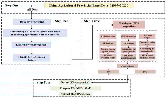
Figure 1.
Research Framework for Agricultural Carbon Emissions in China.
2.4. Dagum Gini Coefficient
Compared with traditional measures such as the Gini coefficient and the Theil index, the Dagum Gini coefficient offers a more comprehensive evaluation of regional disparities. Specifically, it accounts for the distribution characteristics of subsamples and effectively addresses the issue of overlapping among different regional samples. This capability enables it to capture more nuanced cross-regional inequality. Furthermore, the Dagum Gini coefficient allows for the decomposition of total inequality into intra-regional differences, inter-regional differences, and transvariation components, providing deeper insight into the sources of disparity. These advantages make it a superior tool for assessing regional differences in variables such as agricultural carbon emissions or the carbon emissions in agriculture, overcoming the limitations of the traditional Gini coefficient and Theil index [27,28,29]. The specific formula is as follows:
Step one, calculate the overall Gini coefficient G for all provinces.
In the formula, j and h represent different regions, I and r represent different provinces, Q represents the total number of provinces, k represents the total number of regions in one country, represents the average carbon emissions in agriculture in all provinces, and Qj and Qh represent the total number of provinces in j and h respectively.
Step two, calculate the numerical value of Gjj and Gjh, which represent the Gini coefficient in j and the coefficient of j and h.
In the formula, represents the mean value of carbon emissions in agriculture in j province, and represents the mean value of carbon emissions in agriculture in h province.
Step three, calculate the intra-regional gap Gw, inter-regional gap Gb, and super-variable density Gt according to the method of subgroup decomposition.
In the formula, Uj = Qj/Q, ; Djh is the mutual influence of carbon emissions in agriculture between region j and region h. The calculation formula is as follows.
In the formula, djh represents the difference of carbon emissions in agriculture between region j and region h, and Fj and Fh represent the cumulative distribution function of carbon emissions in agriculture in region j and region h.
2.5. Data Sources
The data utilized in this study are sourced from a series of authoritative publications, including the China Statistical Yearbook, China Rural Statistical Yearbook, China Energy Statistical Yearbook, and China Science and Technology Statistical Yearbook, as well as the official website of the National Bureau of Statistics. To enhance regional specificity and data completeness, relevant provincial yearbooks were also consulted. The final panel dataset encompasses 31 provincial-level administrative units in China, including provinces, municipalities, and autonomous regions, covering the period from 1997 to 2022. (Hong Kong, Macau, and Taiwan are excluded due to data availability and statistical standards.) Given the long temporal span, a small number of missing or inconsistent values were identified, primarily resulting from reporting variations and publication lags. This study addressed missing values in certain indicators, such as agricultural tax burden and agricultural R&D investment, by five-year moving average methods for data imputation and smoothing. All data are publicly available and officially published, ensuring the reliability, consistency, and reproducibility of the analysis. In the subsequent research of this study, referring to the classification standards of the National Bureau of Statistics, China is divided into east region, northeast region, central region, and west region in order to better explore the spatiotemporal evolution of agricultural carbon emissions.
3. Measurement and Key Influencing Factors Identification of Agricultural Carbon Emissions in China
3.1. Carbon Emissions Calculation in Agriculture
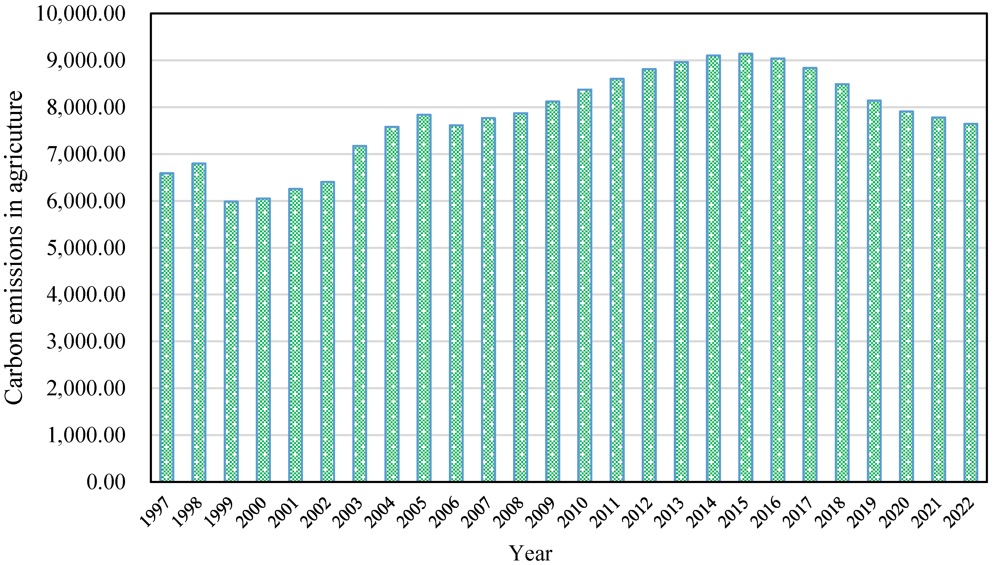
The calculated agricultural carbon emissions in China from 1997 to 2022 are illustrated in Figure 2. This figure presents the national trend of agricultural carbon emissions over the study period, highlighting overall temporal changes. From a long-term perspective, agricultural carbon emissions in China have exhibited a complex and dynamic trajectory. Initially, emissions increased steadily due to the expansion of agricultural production and the intensification of farming practices. However, driven by a combination of stricter environmental policies and technological advancements, emissions began to decline. Despite these improvements, the growing demand for agricultural products has contributed to a renewed upward pressure on emissions, which peaked at 91.415 million tons in 2015. Since then, emissions have gradually declined again. In recent years, increasing emphasis on national food security has intensified pressure on agricultural production. To ensure food supply stability, the use of agricultural inputs such as fertilizers and pesticides has risen, potentially contributing to a partial rebound in emissions.
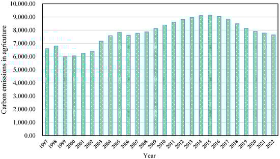
Figure 2.
Agricultural Carbon Emissions in China (Units: 10,000 tons).
Figure 3 presents the violin chart of agricultural carbon emissions across China’s four major regions, including eastern, central, western, and northeastern regions, from 1997 to 2022. The figure displays the distribution and variability of emissions in 4 regions in China, facilitating comparison of regional disparities and changes. The distribution in the eastern regions displays a tall and broad shape, indicating a wide range of emissions. While a substantial portion of the data are concentrated at lower emission levels, the extended upper tail reflects the presence of some high-emission provinces. This significant internal variation suggests diverse agricultural practices and disparities in economic development and technological adoption across the eastern region. In contrast, the central region exhibits a narrow-top, wide-bottom distribution, with most data points clustered around the middle to upper range. The relatively high and consistent level of emissions is likely associated with the region’s role as a major grain production area, characterized by intensive agricultural practices and high input use, including machinery and chemical fertilizers. The western region’s violin plot shows a broader and more dispersed shape, reflecting substantial heterogeneity in emissions. Although the emissions are generally concentrated in the middle-to-lower range, the widespread nature suggests that variations in topography, natural conditions, and farming systems contribute to inconsistent emission levels across the region. Finally, the northeast region features the smallest and most compact distribution, with emissions primarily falling between 0 and 4 million tons. This reflects relatively low and uniform agricultural carbon emissions, likely due to a more homogenous agricultural structure, high technical efficiency, and the prevalence of large-scale, mechanized farming.
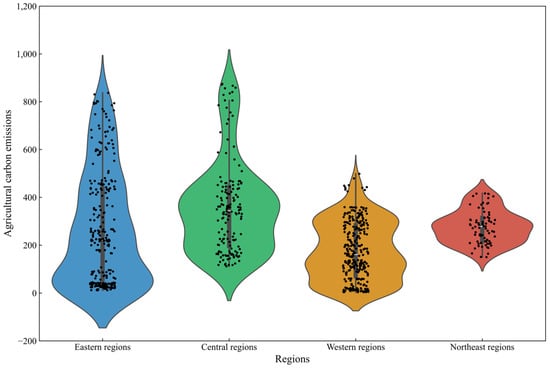
Figure 3.
Violin Chart of Agricultural Carbon Emissions Across China’s Four Major Regions from 1997 to 2022 (Units: 10,000 tons).
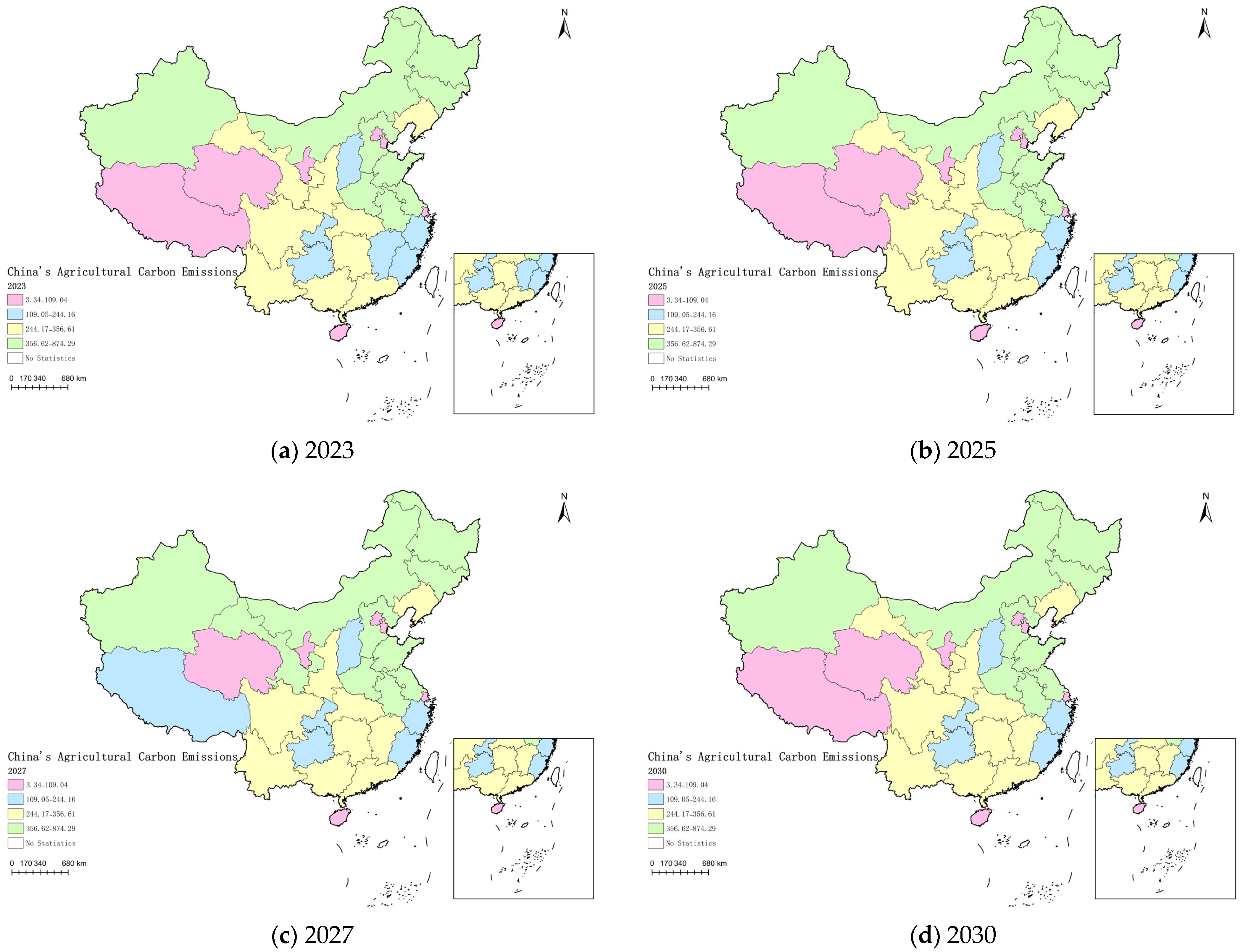
According to the tetrad classification method, China’s agricultural carbon emissions are categorized into four levels, including low [0.0334,1.0904] million tons, medium-low (1.0904,2.4416] million tons, medium-high (2.4416,3.5661] million tons, and high (3.5661,8.7429] million tons. Based on this classification, the spatial distribution of agricultural carbon emissions in the years 1997, 2000, 2005, 2010, 2015, and 2020 was visualized, as illustrated in Figure 4. This map visualizes the spatial distribution and temporal evolution of agricultural carbon emissions across provinces. The results reveal a clear upward trend in emission levels over time. From 1997 to 2020, the number of regions classified as medium-high and high level increased from 4 to 9 and from 6 to 8, respectively. This trend indicates a gradual shift in China’s agricultural carbon emission profile toward higher intensity categories, reflecting mounting pressure on the sector’s environmental performance as agricultural modernization progresses. Meanwhile, the increasing concentration of high-emission regions suggests an urgent need for differentiated and region-specific policy responses. In particular, high- and medium-high emission regions should be subject to more stringent regulatory controls and targeted mitigation measures. This includes promoting low-carbon technologies, improving energy efficiency in agricultural operations, and incentivizing the adoption of sustainable farming practices. Concurrently, a tiered governance approach should be adopted, providing customized support and policy tools based on regional emission profiles to ensure a balanced and effective transition toward low-carbon agricultural development.
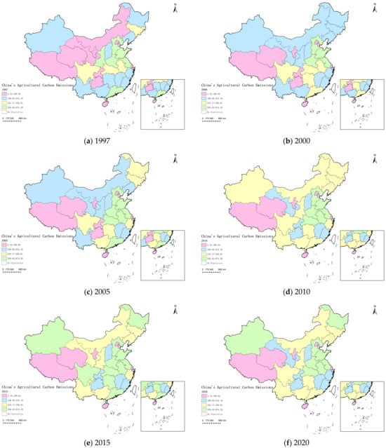
Figure 4.
Spatiotemporal Evolution of Agricultural Carbon Emission Levels in China (Units: 10,000 tons). Map Approval Number: GS (2024) 0650.
3.2. Construction of the Index System for Agricultural Carbon Emissions
This study adopts systems theory as its foundational framework and integrates the PEST theory with the STIRPAT model to construct a multidimensional and dynamic index system for analyzing agricultural carbon emissions. The PEST framework decomposes external environmental drivers across four macro dimensions—political; economic; social; and technological—capturing factors such as agricultural fiscal support (political); industrial structure advancement (economic); rural population density (social); and the level of agricultural mechanization (technological) [9,25]. This integration provides a comprehensive and systematic lens through which the complex, interrelated factors driving agricultural carbon emissions can be analyzed.
Building upon this, the STIRPAT model is employed to quantify the impact of population (P), affluence (A), and technology (T) on environmental degradation (I), expressed through the expanded formula I = aPbAcTd. To enhance explanatory depth, this study incorporates a co-evolutionary perspective of “system-technology-ecology,” introducing additional variables such as urbanization rate and rural education investment (institutional/social) alongside ecological indicators like annual precipitation and forest coverage. This extended model overcomes the traditional STIRPAT framework’s narrow emphasis on technological factors, establishing a more holistic “population-economy-technology-environment” analytical paradigm.
To address the limitations of traditional decomposition and regression models in handling high-dimensional, multicollinear data, Elastic Net Regression is adopted for core variable selection. By combining the sparsity of Lasso and the stability of Ridge, it facilitates the accurate identification of key drivers among 24 candidate variables. Furthermore, machine learning-based feature importance analysis is introduced to rank multidimensional indicators within the PEST-STIRPAT framework, enhancing empirical robustness and validating theoretical assumptions. The specific influencing factors incorporated into the analysis are presented in Table 2.
Table 2.
The Index System of China’s Influencing Factors in Agricultural Carbon Emissions.
Firstly, from the perspective of population and society, this study incorporates key indicators such as agricultural population density and the education level of the agricultural labor force to reflect the allocation and quality of human resources in agricultural production. Additional indicators such as total grain demand, urbanization rate, rural disposable income, and the rural Engel coefficient are selected to capture demographic pressure, consumption patterns, and the socio-economic transformation between rural and urban areas. Secondly, from the economic and industrial dimensions, variables such as the level of agricultural development, fiscal support for agriculture, and investment in agricultural research and education are included to reflect economic capacity and institutional support, while indicators such as industrial structure upgrading, market openness, and agricultural tax burden provide insights into the modernization and competitiveness of the agricultural sector. Thirdly, under the dimensions of technology and production, indicators such as agricultural electricity consumption, total power of agricultural machinery, number of agricultural tools, irrigation security, and the number of green patents are introduced to measure the intensity and efficiency of agricultural inputs, reflecting the role of technological advancement in emission outcomes. Finally, from the standpoint of environmental sustainability, ecological variables such as annual average precipitation, average temperature, forest coverage, and agricultural disaster severity are included to evaluate natural constraints, climate pressures, and their effects on emission volatility and long-term viability. The selection of these indicators is grounded in existing theoretical models, such as STIRPAT and green total factor productivity frameworks, and tailored to the context of China’s agricultural sector. By integrating these multi-dimensional factors, the study constructs a comprehensive evaluation framework aimed at identifying development bottlenecks, informing differentiated policy measures, and providing robust quantitative support for the strategic objectives of high-quality and sustainable agricultural transformation.
3.3. Key Influencing Factors Identification via Elastic Net Regression
In addition to calculating total agricultural carbon emissions, this study standardized all explanatory variables and employed Elastic Net Regression to rank the importance of factors influencing agricultural carbon emissions. Seven key variables were identified, as illustrated in Figure 5. This figure ranks the relative importance of influencing factors based on the Elastic Net Regression model, providing a basis for policy prioritization. Among these, Agricultural Machinery Level (MA) emerged as the most significant determinant, with an importance index of 103.03, substantially higher than that of other variables. This underscores the dominant role of mechanization in driving agricultural carbon emissions in China. Agricultural machinery, predominantly powered by fossil fuels, contributes directly to carbon emissions, particularly in major grain-producing regions. There exists a strong positive correlation between the intensity of mechanical operations and carbon emissions, highlighting the urgent need for emission reductions through clean energy substitution and technological innovation.
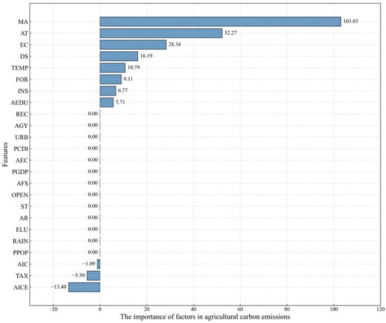
Figure 5.
China’s Key Influencing Factors in Agricultural Carbon Emissions.
Beyond mechanization, several other factors positively promote carbon emissions. These include Numbers of Agricultural Tools (AT), Agricultural Electricity Consumption (EC), Agricultural Disaster Severity (DS), Annual Average Temperature (TEMP), Forest Coverage Rate (FOR), Agricultural Transportation Infrastructure (INS), and Rural Education Investment (AEDU). The quantity of agricultural tools (AT) reflects the scale of capital input in agricultural production. As the deployment of equipment increases, so too does energy consumption during manufacturing, operation, and maintenance, thus exacerbating carbon emissions. Agricultural Electricity Consumption (EC), often associated with irrigation, greenhouse heating, and on-site processing, further amplifies emissions, particularly in regions still dependent on fossil-fuel-based electricity. The agricultural disaster level (DS) indicates the vulnerability of agricultural systems to natural hazards. Post-disaster recovery measures such as replanting, irrigation intensification, and increased use of production inputs can lead to higher energy use and elevated emissions. Rural Education Investment (AEDU), though indirectly linked to emissions, plays a nuanced role. While higher education levels may enhance farmers’ awareness and capacity to adopt low-carbon technologies, such transitions are often delayed by institutional inertia and behavioral lags. Annual Average Temperature (TEMP) acts as a climate-exposure multiplier, increasing evapotranspiration and pest pressure, which in turn escalates input dependency and associated emissions. Unexpectedly, the Forest Coverage Rate (FOR), generally viewed as a carbon sink indicator, may correlate with higher emissions due to land-use displacement effects. Afforestation on marginal lands can push agricultural production toward more intensive practices on remaining arable land, elevating per-unit carbon intensity. Similarly, improvements in Agricultural Transportation Infrastructure (INS), while vital for market connectivity and logistics efficiency, can lock in high-emission pathways through the expansion of cold-chain systems and mechanized distribution, particularly in the absence of green transport solutions.
Conversely, Agricultural Industrial Structure Upgrading (AICE), Agricultural Tax Burden (TAX), and Non-Agricultural Industrial Structure (AIC) exhibit a negative relationship with agricultural carbon emissions. The optimization of industrial structure, such as transitions toward ecological and circular agriculture, reduces reliance on high-carbon inputs and promotes more sustainable production. A higher agricultural tax burden (TAX) may act as a regulatory signal, encouraging producers to internalize environmental costs and adopt more efficient or environmentally friendly practices, which nudges behavioral adjustments and technology substitution over time. Similarly, the expansion of the non-agricultural industrial structure (AIC), particularly through rural labor transfer and the growth of service-oriented or low-emission sectors, can reduce agricultural production intensity by reallocating land and labor resources away from smallholder-based, high-input farming systems. This structural transformation may indirectly contribute to decarbonization by facilitating economies of scale, technological upgrading, and land consolidation, which together improve energy efficiency and reduce emissions per unit of output.
In sum, these findings highlight the multifaceted and dynamic drivers of agricultural carbon emissions. A nuanced understanding of how these variables interact is essential for developing targeted and effective strategies to support the low-carbon transformation of China’s agricultural sector.
4. Model Selection and Prediction in Agricultural Carbon Emissions
4.1. Model Selection and Performance Evaluation for Emission Forecasting
In constructing the SVR model, this study experimented with various kernel functions, including linear, radial basis function (RBF), sigmoid, and polynomial kernels. The results demonstrated that the polynomial kernel significantly outperformed the other options in terms of prediction accuracy. The detailed comparison results are presented in Table 3. The polynomial kernel function exhibits significantly lower Mean Squared Error (MSE) and Mean Absolute Error (MAE) compared to other kernel types, while achieving an R2 value exceeding 0.87, indicating a strong fitting capability. Consequently, the polynomial kernel is selected for subsequent prediction tasks.
Table 3.
Prediction Performance of SVR Models with Different Kernel Functions.
In constructing the RF model, the number of trees was set to 50 to account for the relatively small dataset, and the model was subsequently used to predict the test set. For the BPNN model, a two-hidden-layer architecture was established and trained over 300 epochs using the Adam optimizer and sigmoid activation function. Upon completion of model training, the MSE, MAE, and R2 were calculated. The detailed results are presented in Table 4. As shown, the RF model demonstrated superior predictive performance compared to both SVR and BPNN, achieving a prediction accuracy (R2) of 0.96, thereby rendering it the most suitable model for subsequent forecasting applications.
Table 4.
Prediction Accuracy of Three Machine Learning Models.
After training the high-performing model, this study proceeds to apply algorithmic optimization techniques. Table 5 presents the results of integrating the RF model with GA and PSO. Compared with the baseline results in Table 4, the predictive performance of both optimized models demonstrates noticeable improvement, indicating that the enhanced models possess stronger linear fitting capabilities and are suitable for forecasting agricultural carbon emissions. Notably, the RF model optimized with PSO outperforms the RF-GA model, achieving a lower prediction error and a higher coefficient of determination (R2 = 0.97). Traditional models exhibit significant prediction biases in the presence of missing data or anomalies, whereas RF-PSO optimizes parameters through global search of particle swarm, achieving high prediction accuracy and demonstrating generalization and adaptability in small-sample scenarios, thus providing a reliable basis for policy planning. Based on these results, the RF-PSO model is selected for projecting agricultural carbon emissions across China’s 31 provinces for the period 2023 to 2030.
Table 5.
Prediction Performance of Machine Learning Models with Algorithmic Optimization.
4.2. Results of Forecasting the Carbon Emissions in Agriculture
Based on the currently available data, China’s agricultural carbon emissions can be calculated up to the year 2022. Utilizing Elastic Net Regression, seven key influencing factors were identified. The missing data for these key factors from 2023 to 2030 were supplemented using the five-year moving average method based on recent historical trends. Therefore, the RF-PSO model was employed to predict agricultural carbon emissions for the period from 2023 to 2030, with the results presented in Table 6. The prediction indicates a generally fluctuating but downward trend in China’s agricultural carbon emissions. A minor peak is projected in 2027, with emissions reaching 88.656 million tons, still lower than the peak of 91.415 million tons observed in 2015. This trend suggests that China’s agriculture is currently in a transitional phase toward building carbon neutrality capacity. As the carbon peak and carbon neutrality goals are progressively implemented, agricultural carbon emissions are expected to decline slowly and stabilize over time. These findings are broadly consistent with those of previous studies [6,9].
Table 6.
Prediction Performance of Machine Learning Models with Algorithmic Optimization (Unit: 10,000 tons).
At the provincial level, the forecast shows that agricultural carbon emissions in most regions may experience a minor increase during 2023 to 2028, followed by a fluctuating decline. Notably, carbon emissions in Beijing and Shanghai are projected to remain below 260,000 tons throughout the forecast period. By 2030, agricultural carbon emissions across most provinces are expected to stabilize. However, certain provinces, including Hebei, Heilongjiang, Shandong, Anhui, and Henan, will continue to exhibit relatively high levels of agricultural emissions, each exceeding 4 million tons. As the foundations of China’s agricultural product production, these provinces have a greater demand for inputs such as fertilizers and pesticides in agricultural production, which is a significant reason for the increase in agricultural carbon emissions. Meanwhile, agricultural mechanization has improved production efficiency, but it also means higher fuel consumption. Therefore, it is essential that local governments tailor region-specific policies and interventions to promote the green and low-carbon transformation of agriculture in accordance with local production conditions.
To further illustrate the spatiotemporal dynamics of agricultural carbon emissions in China, this study visualizes the projected emission levels for the years 2023, 2025, 2027, and 2030, as shown in Figure 6. Based on the RF-PSO model, this figure forecasts regional emission trends, contributing to an understanding of pathways toward the carbon peak target. The results indicate a gradual decline in the number of high-emission regions from 9 in 2023 to 3 by 2030, accompanied by a steady increase in regions categorized as low- and medium-low-emission zones. This shift suggests an emerging downward trend in overall agricultural carbon emissions. Meanwhile, the observed pattern may reflect the cumulative impact of China’s sustained efforts in promoting energy conservation, emission reduction, and differentiated regional management strategies. In particular, the implementation of stricter control policies for high-emission regions and tailored guidance for lower-emission areas appears to be yielding tangible results. This transition holds important implications for achieving green and sustainable agricultural development. It demonstrates that with continued optimization of production practices and broader adoption of low-carbon technologies, China’s agricultural sector can further mitigate emissions, ease environmental pressures, and foster a more coordinated trajectory between economic growth and ecological sustainability.
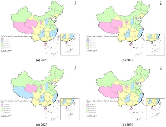
Figure 6.
Spatiotemporal Evolution of Agricultural Carbon Emission Levels in China from 2023 to 2030 (Units: 10,000 tons). Map Approval Number: GS (2024) 0650.
4.3. Analysis of the Sources of Differences in Agricultural Carbon Emissions from 1997 to 2030
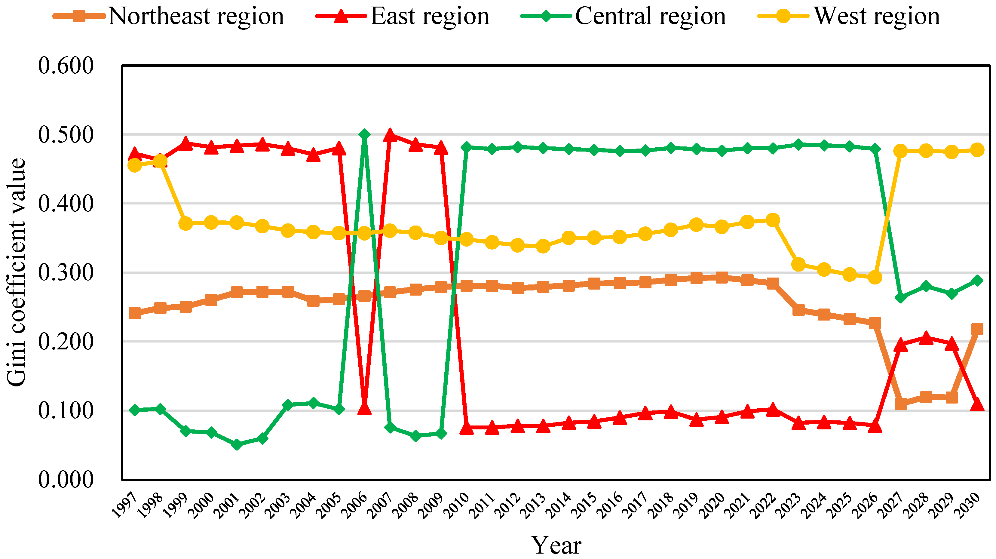
To examine the sources of regional disparities in China’s agricultural carbon emissions from 1997 to 2030, this study employs the Dagum Gini coefficient to decompose overall inequality into intra-regional, inter-regional, and transvariation components. The results of intra-regional disparities are presented in Figure 7. This figure illustrates the internal disparity in emissions within each major region, supporting analysis of regional imbalances. The decomposition reveals dynamic shifts in the dominant regions of internal inequality over time. Specifically, prior to 2009, the Eastern region exhibited the highest intra-regional disparities in agricultural carbon emissions. From 2010 to 2026, this pattern shifted, with the Central region displaying the greatest internal variation. After 2026, the Western region emerged as the region with the highest intra-regional disparity, followed by the Eastern and Central regions. In contrast, the Northeastern region consistently maintained a lower level of internal disparity, indicating relatively homogeneous emission levels across its provinces. These temporal shifts suggest that regional emission disparities are not static but evolve in response to changes in production modes, technological adoption, and policy implementation across space and time.
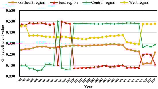
Figure 7.
Subgroup Distribution of Inner-regional Differences in China’s Agricultural Carbon Emissions.
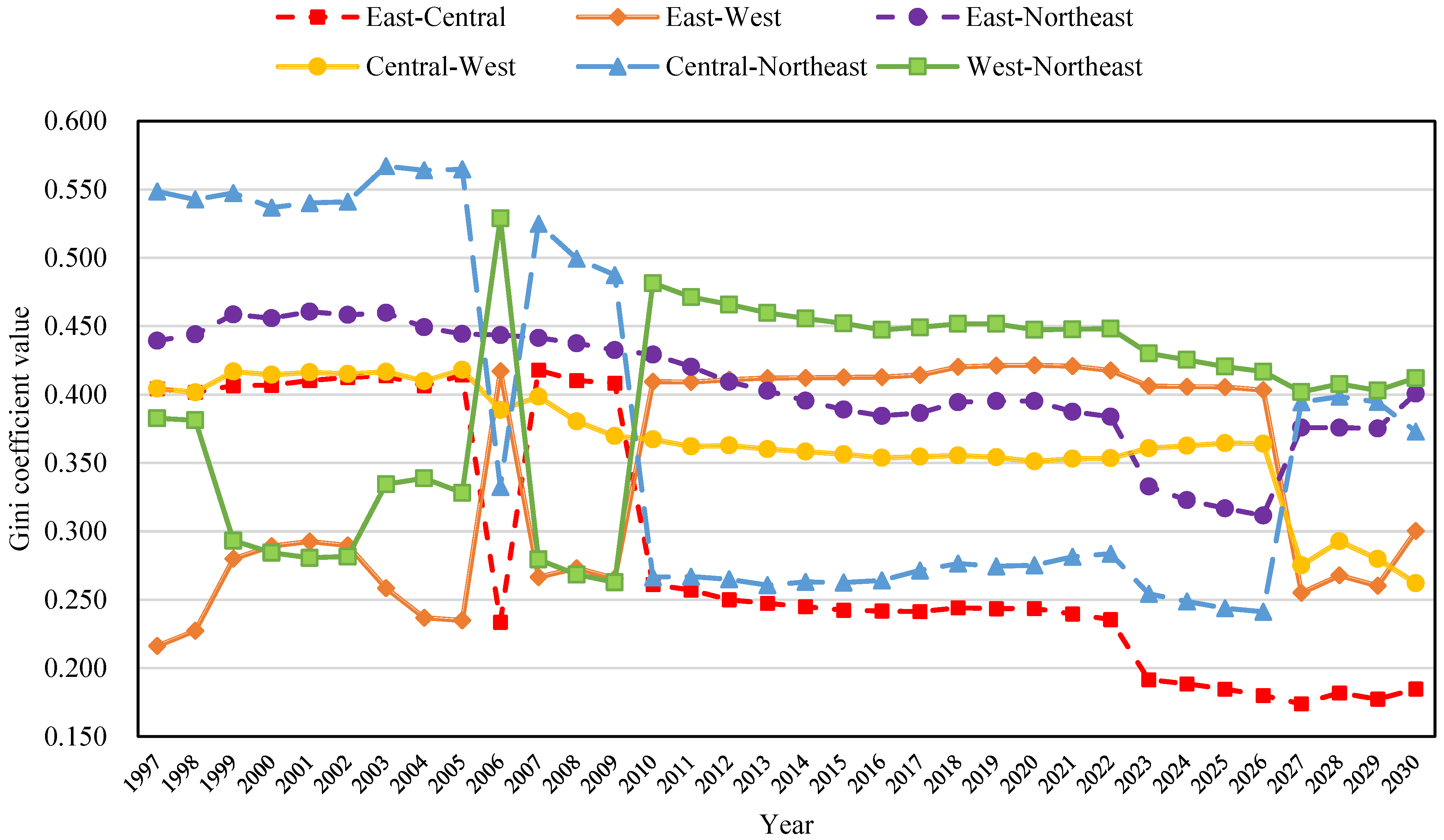
The results of the inter-regional Gini coefficient decomposition are presented in Figure 8. Focusing on between-region variation, this figure shows the evolving structure of emission differences among regional groups. The analysis reveals that inter-regional disparities in agricultural carbon emissions exhibit a fluctuating pattern over time, reflecting evolving spatial dynamics in agricultural development and policy implementation. Among all regional pairings, the most pronounced disparity is consistently observed between the East and Northeast regions, with an average Gini coefficient of 0.406. This substantial gap underscores deep structural differences in agricultural practices, economic development levels, and technological adoption between the more industrialized East and the resource-based Northeast. In contrast, the smallest disparity is found between the Eastern and Central regions, with an average Gini coefficient of 0.288. This suggests a relatively convergent pattern in agricultural emission intensity between these two adjacent regions, likely driven by similar crop structures, comparable mechanization levels, and integrated supply chains facilitated by geographic proximity.
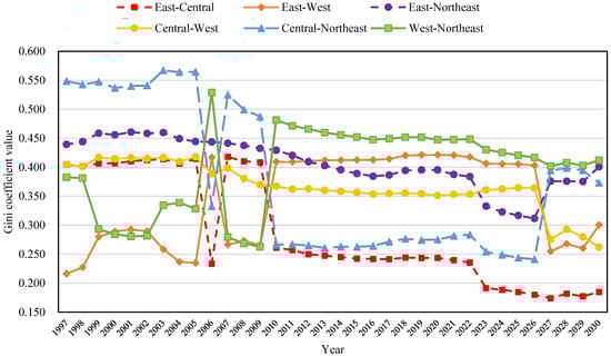
Figure 8.
Subgroup Distribution of Inter-regional Differences in China’s Agricultural Carbon Emissions.
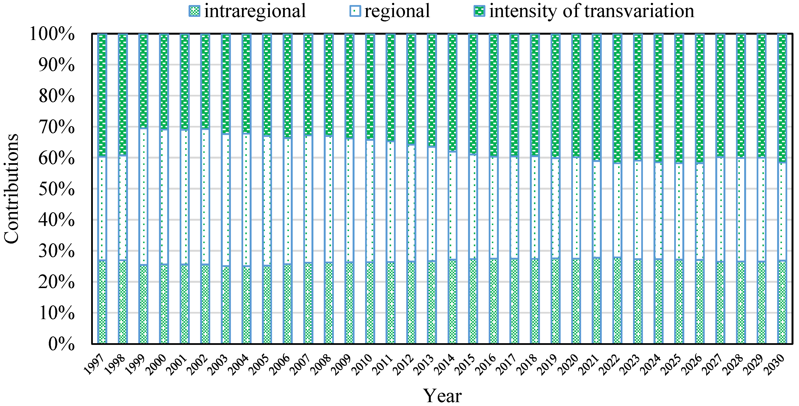
The differential contribution rates of agricultural carbon emissions across China’s four major regions from 1997 to 2030 are illustrated in Figure 9. Using Dagum Gini coefficient decomposition, this figure presents the dynamic contributions of intra-regional, inter-regional, and transvariation density components to overall emission disparity. The decomposition of inequality sources reveals that super-variable density, which reflects the degree of overlap in emission distributions across regions, accounts for an average of 37.078% of the total Gini coefficient. This indicates that a substantial portion of spatial inequality arises not from distinct regional clusters but from cross-regional heterogeneity and intersecting emission levels. Furthermore, the dominant source of agricultural carbon emission disparities shifted over time. Between 1999 and 2013, inter-regional differences were the primary contributor to overall inequality, suggesting relatively stable, region-specific emission patterns during that period. However, after 2013, super-variable density emerged as the predominant source of disparity, highlighting a growing complexity in the spatial dynamics of agricultural carbon emissions. This reflects the complex and interwoven nature of China’s agricultural development patterns.
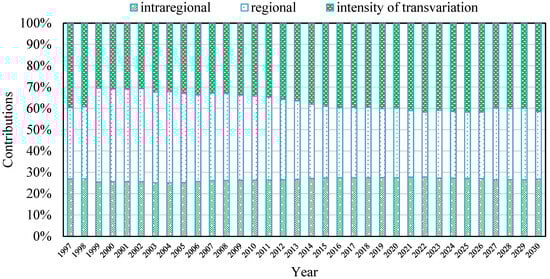
Figure 9.
Differential Contribution Trend in China’s Agricultural Carbon Emissions.
5. Discussion
From a systems perspective, agricultural carbon emissions in China should be understood not merely as the sum of input-based activities, but as the outcome of dynamic interactions among technological infrastructure, institutional arrangements, behavioral incentives, and environmental constraints. This study reveals that the agricultural emission system exhibits strong structural imbalances, nonlinear feedbacks, and regionally differentiated subsystem features that cannot be captured through linear or reductionist approaches.
5.1. The Foundational Profile of Agricultural Carbon Emissions in China
Between 1997 and 2022, China’s agricultural carbon emissions exhibited a clear structural pattern. This finding is consistent with Zhang et al. [9], who identified fertilizers and agricultural diesel as the primary contributors, supporting the IPCC assertion that carbon emissions in agriculture are predominantly driven by production input intensity. However, this study further reveals the often-overlooked role of “hidden” carbon sources, such as pesticides and plastic mulch films. Although these auxiliary inputs are used in relatively small quantities, their cumulative carbon footprint across production, transportation, application, and disposal phases can be substantial, particularly given their widespread use in modern crop production. Traditional life cycle assessment (LCA) approaches often fail to account for these emissions, indicating a methodological gap in capturing full-cycle environmental impacts in agriculture. These findings underscore the need for a more comprehensive and nuanced approach to agricultural carbon accounting, one that includes indirect emissions from auxiliary materials and highlights the importance of region-specific mitigation strategies. Promoting the adoption of low-emission feed technologies, especially in high-risk regions such as Northeast China, and incorporating hidden emission sources into national carbon inventories will be essential steps toward a more systemic and accurate management of agricultural emissions.
5.2. The Influencing Key Factors and Interactions in China’s Agricultural Carbon Emissions
In the identification of key influencing factors of agricultural carbon emissions, this study finds that Agricultural Machinery Level (MA), Number of Agricultural Tools (AT), Agricultural Electricity Consumption (EC), Agricultural Disaster Severity (DS), and Agricultural Industrial Structure Upgrading (AICE) are the top five determinants. This highlights the combined influence of input intensity, structural transition, and technology application modes in shaping emission patterns. These findings are consistent with Aguilera et al. [30], who emphasized the significant contribution of mechanization to emission growth. The dominance of mechanization-related variables (MA, AT, EC) signals China’s continued transition toward capital-intensive agriculture. However, this transition is unfolding without sufficient institutional support for clean energy integration or machinery-sharing systems, resulting in a path-dependent lock-in to fossil-fuel-based practices. This points to a structural inefficiency wherein the physical expansion of mechanization is not matched by ecological modernization or system-level energy reform. Furthermore, the observed impact of Agricultural Disaster Severity (DS) suggests that environmental shocks exacerbate emissions through reactive input intensification, underlining the need for climate-resilient agricultural strategies [31].
Moreover, the limited effectiveness of Rural Education Investment (AEDU) in curbing emissions highlights a crucial disconnect between knowledge provision and behavioral transformation. Importantly, this study extends the traditional STIRPAT framework by revealing a nonlinear relationship between technological input, particularly green innovation metrics such as the number of green patents, and agricultural carbon emissions. In addition, institutional variables such as Agricultural Tax Burden (TAX) and the share of Non-Agricultural Industrial Structure (AIC) reveal potential indirect emission mitigation pathways. Taxation, as a regulatory instrument, can signal the internalization of environmental externalities, nudging producers toward more efficient input use. Meanwhile, the structural shift toward non-agricultural sectors facilitates labor migration and land consolidation, indirectly lowering emission intensity by transforming traditional smallholder production modes. Taken together, these findings demonstrate that agricultural carbon emissions are emergent properties of an interconnected system comprising technology, institutions, environment, and behavior. Effective emission reduction therefore requires coordinated interventions across these domains, leveraging structural reforms, behavioral insights, and innovation ecosystems to trigger systemic transitions toward low-carbon agriculture.
5.3. Modeling Agricultural Emissions in Complex Systems
In the domain of predictive modeling, the superior performance of the RF-PSO hybrid model (R2 = 0.97) is not solely attributed to the advantages of ensemble learning. Rather, it reflects the model’s capacity to capture the complex nonlinear interdependencies among variables influencing agricultural carbon emissions. Compared to traditional regression techniques, this hybrid model leverages Particle Swarm Optimization (PSO) to dynamically adjust feature weights within the input space, thereby significantly mitigating the risk of overfitting. It also excels in identifying nonlinear variable interactions, ultimately enhancing both prediction accuracy and generalizability. These findings align with Xia et al. [3], who emphasized that multi-model integration substantially improves forecasting stability and robustness. Importantly, the underperformance of SVR and BPNN when confronted with high-dimensional, imbalanced feature sets underscores their limited adaptability to heterogeneous agricultural data. SVR tends to be sensitive to skewed distributions and outliers, often converging to suboptimal solutions. Similarly, BPNN suffers from instability in convergence due to its sensitivity to initial parameter settings and inherent randomness in training, making it less reliable in complex, noisy datasets. In contrast, the PSO algorithm demonstrates superior optimization performance due to its enhanced global search capacity and faster convergence speed. Unlike Genetic Algorithm (GA), which is prone to premature convergence in early iterations, PSO is better equipped to explore the parameter space efficiently and avoid local minima. This indicates that optimization algorithms should not be treated as peripheral components but rather as integral elements in the system modeling architecture. Their design and selection directly impact the robustness and scalability of forecasting models, particularly in high-dimensional and nonlinear contexts such as agricultural carbon modeling. Overall, the RF-PSO model not only delivers strong predictive capability but also provides a reproducible and scalable solution framework for addressing complex, high-dimensional agricultural data challenges. Future modeling efforts can build upon this foundation by integrating dynamic feature selection mechanisms and time-series modeling approaches to develop more interpretable, mechanism-informed predictive systems. However, as a supervised learning model, RF-PSO has three notable limitations. First, it relies heavily on large volumes of labeled data, making it difficult to detect unlabeled or rare patterns such as extreme climate events. Second, the model assumes spatial homogeneity, which limits its ability to capture heterogeneous interactions between high-emission eastern provinces and low-emission regions in western China. Third, RF-PSO lacks dynamic clustering capabilities, hindering its effectiveness in identifying shifting regional emission patterns, especially in the context of the projected 2027 emission peak. In addition to these structural limitations, it is also important to recognize the inherent uncertainty associated with forecasting future agricultural carbon emissions. Exogenous shocks such as abrupt policy shifts, breakthrough technologies, or extreme climate events may substantially alter emission trajectories in ways that supervised learning models trained solely on historical data may not fully capture. Moreover, the current model does not incorporate scenario-based simulations or sensitivity analysis to account for alternative policy intensities, structural transitions, or the varying adoption rates of green technologies. Future research could incorporate unsupervised learning methods (e.g., K-Means) to enable dynamic clustering of emission patterns across China’s 31 provinces or apply Geographically Weighted Regression (GWR) to uncover the spatially non-stationary relationships among key influencing factors, thereby providing a more granular and region-specific policy design framework. Additionally, scenario-based forecasting approaches, such as constructing low, medium, and high emission-reduction policy scenarios, and techniques like Monte Carlo simulations or Bayesian networks could be employed to assess the robustness of predictions under varying assumptions. These additions would improve the model’s adaptability and provide a more nuanced understanding of potential future emission pathways.
5.4. Imbalance and Gaps in Regional Emission Disparities
This study employs the Dagum Gini coefficient decomposition to systematically assess regional disparities in China’s agricultural carbon emissions, revealing that transvariation accounts for the largest proportion of inequality at 37.078%. This indicates that carbon emissions across regions are not only uneven but significantly overlapping, underscoring structural issues such as asynchronous technology diffusion, inconsistent policy implementation, and fragmented allocation of key production factors like labor, capital, and land. From a regional perspective, the eastern region benefits from mature agricultural infrastructure, digital management platforms, and responsive policy frameworks that support machinery sharing and standardized operations, leading to more efficient carbon control. In contrast, the central and western regions face several systemic constraints, including limited fiscal capacity, underdeveloped transportation and digital infrastructure, and weakly organized farming structures. These barriers hinder the widespread adoption and scaling of green agricultural technologies. Moreover, the coexistence of disparate production entities, large-scale commercial farms, and smallholder households within the same region exacerbates intra-regional inequalities. For example, while some modern farms in Heilongjiang have achieved mechanization rates exceeding 90%, several counties in neighboring Jilin province still rely on traditional, labor-intensive farming practices. This illustrates a critical misalignment between technological availability and the capacity for its effective implementation. Such structural imbalances weaken the overall coherence of national emission reduction strategies and reduce the potential for synergistic regional outcomes. To address these disparities, there is an urgent need to establish cross-regional collaboration frameworks for agricultural carbon governance. Examples include developing interprovincial agricultural machinery sharing platforms, creating regional low-carbon agriculture demonstration corridors, and constructing real-time agricultural carbon monitoring networks. These mechanisms would help overcome administrative silos, enabling more integrated resource allocation and technology diffusion. Furthermore, emission reduction policies should be tailored to reflect regional heterogeneity in terms of economic capacity, industrial structure, and ecological endowments. By designing differentiated, context-sensitive support mechanisms, policymakers can better align national carbon neutrality goals with localized developmental realities, thereby promoting a more adaptive and system-oriented approach to agricultural decarbonization.
Compared to existing studies that primarily focus on static or single-dimensional analyses of agricultural carbon emissions, this study advances the literature in several key aspects. First, it employs a comprehensive indicator system that integrates economic, social, technological, and environmental dimensions, enabling a more holistic understanding of emission drivers. Second, the use of Elastic Net Regression enhances variable selection accuracy in the presence of multicollinearity, which is a common challenge in high-dimensional agricultural datasets, an improvement over traditional regression-based decomposition methods. Third, this study incorporates a hybrid RF-PSO model for emission forecasting, which demonstrates superior accuracy and interpretability in nonlinear systems compared to conventional models like SVR or BPNN. Fourth, by applying the Dagum Gini coefficient to decompose regional disparities, this study captures the dynamic evolution of intra-regional, inter-regional, and transvariation components over a long temporal horizon, offering a novel spatial inequality perspective rarely explored in prior research. Finally, the research proposes actionable governance mechanisms such as cross-provincial machinery sharing and carbon monitoring networks to bridge implementation gaps, an area often overlooked in purely theoretical studies. These contributions collectively extend both the methodological toolkit and policy applicability of agricultural carbon emission research in China.
6. Conclusions and Implications
The study employs elastic net regression to identify the key drivers of agricultural carbon emissions in China, systematically evaluates the predictive performance of machine learning models including Random Forest (RF), Support Vector Regression (SVR), and Backpropagation Neural Network (BPNN), and further enhances model performance using Genetic Algorithm (GA) and Particle Swarm Optimization (PSO). Based on the optimal model, agricultural carbon emissions from 2023 to 2030 are forecasted, and regional disparities are assessed through Dagum Gini coefficient decomposition. The main findings are as follows:
Firstly, elastic net regression was applied to screen 24 influencing factors, identifying eleven key variables affecting agricultural carbon emissions, including Agricultural Machinery Level (MA), Numbers of Agricultural Tools (AT), Agricultural Electricity Consumption (EC), Agricultural Disaster Severity (DS), Annual Average Temperature (TEMP), Forest Coverage Rate (FOR), Agricultural Transportation Infrastructure (INS), Rural Education Investment (AEDU), Agricultural Industrial Structure Upgrading (AICE), Agricultural Tax Burden (TAX), and Non-Agricultural Industrial Structure (AIC). Among them, MA, AT, EC, DS, and AICE ranked as the top five in terms of importance, emphasizing the critical role of mechanization and industrial transition in emission dynamics.
Secondly, the prediction performance of RF, SVR, and BPNN models was compared using MSE, MAE, and R2 as evaluation metrics. RF demonstrated superior performance with an R2 of 0.96. Further optimization using GA and PSO enhanced prediction accuracy, with the RF-PSO hybrid model achieving the best results, thereby confirming the robustness of ensemble learning combined with metaheuristic optimization in modeling complex nonlinear systems.
Thirdly, from 1997 to 2030, China’s agricultural carbon emissions exhibited a fluctuating pattern, with a peak of 91.415 million tons in 2015. Although recent years show signs of a rebound, forecasts predict a minor peak in 2027 followed by a gradual decline and eventual stabilization. At the provincial level, most regions are expected to reach small peaks between 2023 and 2028, with emissions becoming relatively stable by 2030. However, provinces such as Hebei, Heilongjiang, Shandong, Anhui, and Henan will continue to record high emission levels, each exceeding 4 million tons.
Lastly, spatial disparity analysis using the Dagum Gini coefficient reveals a declining but persistent imbalance in regional emissions. The overall Gini coefficient trends downward over the study period, yet hypervariable density accounts for the largest share of inequality, averaging 37.08%. This suggests significant cross-regional spillover effects due to differences in technology diffusion, policy implementation, and resource allocation, underlining the need for enhanced regional coordination to achieve low-carbon agricultural development. This section is not mandatory but can be added to the manuscript if the discussion is unusually long or complex.
Based on the above-mentioned research conclusions, the implications are as follows. Firstly, China’s government should enhance cross-regional coordination in emission reduction. The dominance of hypervariable density in regional disparities suggests significant overlaps across China’s four main regions. Establishing collaborative platforms for technology sharing, joint monitoring, and differentiated regional targets can improve policy coherence and emission reduction effectiveness. For example, through the technology-sharing mechanism, the integrated pesticide and fertilizer technology will be transferred to the major agricultural provinces with high carbon emissions; at the same time, a joint monitoring network will be built to integrate the cross-border emission data of agricultural plastic film-intensive areas. Then, China’s government should invest in high-quality agricultural human capital. As Rural Education (AEDU) strongly influences emissions, strengthening agricultural education and vocational training, especially in digital and low-carbon technologies, will foster a skilled labor force aligned with modern, low-emission practices. In addition, priority should be given to providing subsidized skill-upgrading projects for high-emission areas to train professional teams adapted to green production. Meanwhile, China’s government should accelerate adoption of low-carbon technologies and sustainable practices. Key influencing factors such as Machinery Level (MA) and input intensity highlight the need for promoting energy-efficient equipment, reducing chemical input use, and supporting ecological agriculture to cut emissions without compromising food security. Accordingly, it is recommended that high-emission provinces such as Hebei and Shandong establish cross-provincial agricultural machinery sharing platforms. These platforms should integrate advanced electric agricultural machinery from eastern regions with the large-scale farming experience of the Northeast, thereby improving resource allocation efficiency and reducing carbon emissions effectively. Finally, a data- and AI-driven monitoring system was built. The RF-PSO model performed well in prediction. Statistical, satellite, and Internet of Things data were integrated into the real-time monitoring platform, and early warning systems were deployed first in the top 10% of provinces with agricultural carbon emissions, providing a basis for provincial precision policy formulation.
7. Limitations and Reflection
This study focuses on identifying key influencing factors and predicting agricultural carbon emissions using machine learning models, yet several limitations persist. To begin with, data inconsistencies and missing values required interpolation. Because a moving average method was used to handle a small portion of missing yearly data. While this approach helps maintain temporal smoothness in the dataset, it estimates missing values based on neighboring years’ averages, which may fail to capture sudden agricultural shocks or structural changes. As a result, the model’s predictive performance may be weakened in abnormal or extreme years, particularly when key variables experience significant fluctuations. Additionally, the moving average may introduce smoothing bias, potentially obscuring real dynamic trends and affecting the identification of variable relationships and model interpretability. This limitation underscores the importance of enhancing the timeliness and completeness of agricultural carbon emission data in future research, as well as incorporating more flexible preprocessing techniques to improve model robustness and adaptability. Secondly, the model assumes stable relationships and excludes climate shocks or carbon sink effects, reducing prediction accuracy during extreme events. Then, only supervised learning models (e.g., RF, SVR, BPNN) were applied, while unsupervised methods such as K-Means were not used, limiting the model’s ability to dynamically cluster regions and explore evolving emission patterns. Lastly, spatial heterogeneity in technological diffusion was not fully captured, as variation in technology adoption across regions remains unquantified.
Future research will consider integrating Structural Equation Modeling (SEM) or combining RF-PSO with interpretable machine learning techniques such as SHAP to better explore the dynamic relationships and potential offsetting effects among key influencing factors. In addition, future studies should enhance data granularity by incorporating detailed variables such as energy types and irrigation methods. Climate indicators and carbon sink modules should be included to construct a dynamic emission-sequestration model. Policy simulation can help evaluate regional transitions under China’s “dual carbon” goals. Finally, integrating unsupervised methods like K-Means and spatial econometric techniques such as geographically weighted regression (GWR) will improve regional clustering, support adaptive policy design, and increase prediction robustness.
Author Contributions
J.L., Writing—original draft; Writing—review and editing; Methodology; Conceptualization; Resources. X.P., Data curation; Investigation; Formal analysis. J.Z., Writing—original draft; Data curation; Investigation; Supervision; Formal analysis. Y.M., Writing—review and editing; Data curation. C.J., Writing—review and editing; Investigation; Data curation; Validation. W.H., Writing—review and editing; Resources; Visualization. M.H., Writing—original draft; Writing—review and editing; Methodology; Conceptualization; Supervision; Validation; Project administration. All authors have read and agreed to the published version of the manuscript.
Funding
This research was funded by the Humanities and Social Sciences Youth Fund Project of the Ministry of Education (number 24YJC790065), the National Key Research and Development Program of China project (number 2021YFF0601005), and the Ministry of Education’s Chunhui Plan (number HZKY20220346).
Data Availability Statement
The datasets used and/or analyzed during the current study are available from the corresponding author on reasonable request.
Conflicts of Interest
Author Wanling Hu was employed by the company China Carbon Emissions Registration and Clearing Co., Ltd. The remaining authors declare that the research was conducted in the absence of any commercial or financial relationships that could be construed as a potential conflict of interest.
References
- Jones, M.W.; Peters, G.P.; Gasser, T.; Andrew, R.M.; Schwingshackl, C.; Gütschow, J.; Houghton, R.A.; Friedlingstein, P.; Pongratz, J.; Le Quéré, C. National contributions to climate change due to historical emissions of carbon dioxide, methane, and nitrous oxide since 1850. Sci. Data 2023, 10, 155. [Google Scholar] [CrossRef] [PubMed]
- Zheng, J.; Duan, H.; Zhou, S.; Wang, S.; Gao, J.; Jiang, K.; Gao, S. Limiting global warming to below 1.5 °C from 2 °C: An energy-system-based multi-model analysis for China. Energy Econ. 2021, 100, 105355. [Google Scholar] [CrossRef]
- Xia, X.; Liu, B.; Wang, Q.; Luo, T.; Zhu, W.; Pan, K.; Zhou, Z. Analysis of carbon peak achievement at the provincial level in China: Construction of ensemble prediction models and Monte Carlo simulation. Sustain. Prod. Consum. 2024, 50, 445–461. [Google Scholar] [CrossRef]
- Hu, Y.; Su, M.; Jiao, L. Peak and fall of China’s agricultural GHG emissions. J. Clean. Prod. 2023, 389, 136035. [Google Scholar] [CrossRef]
- Chen, Y.; Miao, J.; Zhu, Z. Measuring green total factor productivity of China’s agricultural sector: A three-stage SBM-DEA model with non-point source pollution and CO2 emissions. J. Clean. Prod. 2021, 318, 128543. [Google Scholar] [CrossRef]
- Yu, Y.; Jiang, T.; Li, S.; Li, X.; Gao, D. Energy-related CO2 emissions and structural emissions’ reduction in China’s agriculture: An input–output perspective. J. Clean. Prod. 2020, 276, 124169. [Google Scholar] [CrossRef]
- Bamber, N.; Johnson, R.; Laage, E.; Dias, G.; Tyedmers, P.; Pelletier, N. Life cycle inventory and emissions modelling in organic field crop LCA studies: Review and recommendations. Resour. Conserv. Recycl. 2022, 185, 106465. [Google Scholar] [CrossRef]
- Xie, T.; Huang, Z.; Tan, T.; Chen, Y. Forecasting China’s agricultural carbon emissions: A comparative study based on deep learning models. Ecol. Inform. 2024, 82, 102661. [Google Scholar] [CrossRef]
- Zhang, X.; Liu, C.; Zhang, J.; Liu, J.; Hu, W. Evolution Trends in Carbon Emissions and Sustainable Development Paths in China’s Planting Industry from the Perspective of Carbon Sources. Sustainability 2025, 17, 2772. [Google Scholar] [CrossRef]
- Feng, J.; Li, H.; Cannon, N.; Chang, X.; Chu, Q. A Simulation Study of How Chinese Farmer Cooperatives Can Drive Effective Low-Carbon Production Systems Through a Carbon Transaction Incentive. Systems 2025, 13, 260. [Google Scholar] [CrossRef]
- Hao, D.; Wang, R.; Gao, C.; Song, X.; Liu, W.; Hu, G. Spatial-Temporal Characteristics and Influence Factors of Carbon Emission from Livestock Industry in China. Int. J. Environ. Res. Public Health 2022, 19, 14837. [Google Scholar] [CrossRef] [PubMed]
- Ma, S.; Li, J.; Wei, W. The carbon emission reduction effect of digital agriculture in China. Environ. Sci. Pollut. Res. 2022, 53, 102473. [Google Scholar] [CrossRef]
- Bai, J.; Wang, Y.; Sun, W. Exploring the role of agricultural subsidy policies for sustainable agriculture Based on Chinese agricultural big data. Sustain. Energy Technol. Assess. 2022, 53, 102473. [Google Scholar] [CrossRef]
- Gao, Y.; Zhang, M.; Wang, K.; Wen, F.; Liu, F. The Carbon Emissions Reduction Effect of Green Agricultural Subsidy Policy: A Quasi-Natural Experiment. Sustainability 2024, 16, 5210. [Google Scholar] [CrossRef]
- Robinson, A.; Lehmann, J.; Barriopedro, D.; Rahmstorf, S.; Coumou, D. Increasing heat and rainfall extremes now far outside the historical climate. npj Clim. Atmos. Sci. 2021, 4, 45. [Google Scholar] [CrossRef]
- Xiong, C.; Yang, D.; Xia, F.; Huo, J. Changes in agricultural carbon emissions and factors that influence agricultural carbon emissions based on different stages in Xinjiang, China. Sci. Rep. 2016, 6, 36912. [Google Scholar] [CrossRef]
- Yang, L.; Liu, X.; Kang, X.; Zhu, Y.; Wu, C.; Liu, B.; Li, W. Coupling Agricultural Carbon Emission Efficiency and Economic Growth: Evidence from Jiangxi Province, China. Sustainability 2025, 17, 4246. [Google Scholar] [CrossRef]
- Fan, J.; Lv, J.; Qi, L. Sparse High-Dimensional Models in Economics. Annu. Rev. Econ. 2011, 3, 291–317. [Google Scholar] [CrossRef]
- Xu, Y.; Fan, Y.; Yeh, C.H.; Zhang, L. A Machine Learning-Based Approach to Identifying Key Innovation Determinants for Industrial Firms: The Case of the Pharmaceutical Industry in China. IEEE Trans. Eng. Manag. 2024, 71, 6103–6115. [Google Scholar] [CrossRef]
- Ram, M.; Bracci, E.; Nizamani, B. Achievements of Waste Indicators of Sustainable Development Goals 6, 7, 11, and 12 in Italy from 2015 to 2020. Sustainability 2025, 17, 3952. [Google Scholar] [CrossRef]
- Huang, Y.; Shen, L.; Liu, H. Grey relational analysis, principal component analysis and forecasting of carbon emissions based on long short-term memory in China. J. Clean. Prod. 2019, 209, 415–423. [Google Scholar] [CrossRef]
- Wang, H.; Jin, Y.; Hong, X.; Tian, F.; Wu, J.; Nie, X. Integrating IPAT and CLUMondo Models to Assess the Impact of Carbon Peak on Land Use. Land 2022, 11, 573. [Google Scholar] [CrossRef]
- Karamdel, H.; Ashtiani, M.; Mehditabar, M.J.; Bakhshi, F. A consensus-based approach to improve the accuracy of machine learning models. Evol. Intell. 2024, 17, 4257–4278. [Google Scholar] [CrossRef]
- Wang, L.; Shi, P.; Luo, J.; Yin, J.; Cheng, F.; Shi, J.; Wang, Z. Region-county characteristics of spatiotemporal dynamic evolution and influencing factors on agricultural net carbon sink in Hexi region of Gansu Province. Ecol. Indic. 2024, 169, 112817. [Google Scholar] [CrossRef]
- Zhang, J.; Peng, X.; Zhang, J.; Liu, J.; Hu, W. Stage characteristics, spatial differences and dynamic evolution of crop carbon sink in Hubei Province based on the crop data from 1997 to 2022. J. Environ. Eng. Technol. 2024, 14, 1513–1522. [Google Scholar]
- Zhao, H.; Jia, X.; Yang, J.; Wu, Y.; Wu, X.; Du, L. Spatiotemporal variations and influencing factors of methane emissions from livestock in China: A spatial econometric analysis. Sci. Total Environ. 2024, 931, 173010. [Google Scholar] [CrossRef]
- Mai, Q.; Bai, M.; Li, L. Study on the Dynamic Evolution and Regional Differences of the Level of High-Quality Economic and Social Development in China. Sustainability 2023, 15, 382. [Google Scholar] [CrossRef]
- Zha, Q.; Liu, Z.; Song, Z.; Wang, J. A study on dynamic evolution, regional differences and convergence of high-quality economic development in urban agglomerations: A case study of three major urban agglomerations in the Yangtze river economic belt. Front. Environ. Sci. 2022, 10, 1012304. [Google Scholar] [CrossRef]
- Lv, C.; Bian, B.; Lee, C.-C.; He, Z. Regional gap and the trend of green finance development in China. Energy Econ. 2021, 102, 105476. [Google Scholar] [CrossRef]
- Aguilera, E.; Guzmán, G.I.; González De Molina, M.; Soto, D.; Infante-Amate, J. From animals to machines. The impact of mechanization on the carbon footprint of traction in Spanish agriculture: 1900–2014. J. Clean. Prod. 2019, 221, 295–305. [Google Scholar] [CrossRef]
- Wang, S.; Bai, X.; Zhang, X.; Reis, S.; Chen, D.; Xu, J.; Gu, B. Urbanization can benefit agricultural production with large-scale farming in China. Nat. Food 2021, 2, 183–191. [Google Scholar] [CrossRef] [PubMed]


Disclaimer/Publisher’s Note: The statements, opinions and data contained in all publications are solely those of the individual author(s) and contributor(s) and not of MDPI and/or the editor(s). MDPI and/or the editor(s) disclaim responsibility for any injury to people or property resulting from any ideas, methods, instructions or products referred to in the content. |
© 2025 by the authors. Licensee MDPI, Basel, Switzerland. This article is an open access article distributed under the terms and conditions of the Creative Commons Attribution (CC BY) license (https://creativecommons.org/licenses/by/4.0/).