Abstract
Amidst escalating concerns about climate change, manufacturers are increasingly pressured to adopt a low-carbon supply chain (LCSC). Financial constraints deter numerous companies from embracing low-carbon initiatives in a competitive landscape. Inclusive internal financing (IIF) provides operational funds from capital-abundant members to capital-constrained members, resolving funding shortages internally within the system. However, when dominant members cannot support all such enterprises, selective internal financing (SIF) or hybrid financing (HF) becomes necessary. This paper studies the operation and financing strategies of a competitive LCSC. Within the framework of an LCSC where two capital-constrained retailers compete, using Stackelberg game theory and the backward induction method, three game-theoretical models are developed under IIF, SIF, and HF. The results indicate that increased competition intensity reduces product sales price, the manufacturer’s carbon emission reduction level, and profit. When competition intensity is high, SIF more effectively enhances carbon emission reduction level, product sales quantity, and profit acquisition. HF reduces profits for the allied retailer and diminishes its competitiveness, yet enhances the competitive strength of the rival retailer. Numerical analysis demonstrates that when equity financing in HF exceeds 0.546, the allied retailer becomes unprofitable and is driven out of the market. This study complements LCSC finance research and provides references for supply chain operations and financing strategy formulation.
1. Introduction
With the increasing concern over climate change and ecological sustainability, low-carbon supply chain (LCSC) systems have emerged. China’s 2030 Carbon Peak Action Plan clearly requires manufacturing enterprises to achieve emission reduction targets through systematic measures such as cleaner production transformation, energy management center construction, and comprehensive resource utilization. Meanwhile, enterprises have responded with innovations, such as the “zero carbon source” air conditioning technology jointly developed by GREE and Tsinghua University. These developments indicate that the LCSC is transforming from policy-driven to market-driven initiatives, becoming a catalyst for manufacturing industry transformation and green economy integration. However, in LCSC systems, individual entities (such as small retailers) frequently encounter financial obstacles during operations. Furthermore, peer retailers face competition when targeting the same market, hindering the sustainable operation of the system. The interaction between retailers’ financial constraints and market competition significantly amplifies the operational complexity of the LCSC system. In this context, a key scientific question remains unresolved: within competitive LCSCs where capital-constrained retailers coexist, what financing mode can enhance system resilience and achieve sustainable the operation of LCSC systems? This is an interesting and worthy research problem.
Specifically, facing the intertwined challenges of retailers’ capital constraints and competition, providing financial support to retailers emerges as a critical solution [1,2]. For instance, Linklogis utilizes fully digitalized supply chain finance technology to significantly reduce resource consumption and carbon emissions within supply chain operations. As of 2024, the company has cumulatively provided inclusive financing and selective financing to over 330,000 SMEs. Through digital tools, it has reduced financing costs by 30–50%, markedly improving supply chain financing efficiency [3]. Existing research has demonstrated that financing mechanisms enhance the return on investment for small and medium-sized retailers, while disparities in financing strategies directly shape market competition patterns and supply chain stability [4,5]. In analysis within the framework of supply chain systems, financing modes include inclusive internal financing (IIF), selective internal financing (SIF), and hybrid financing (HF) [6,7]. Specifically, IIF refers to a financing model where capital-constrained members do not rely on external financing. The supply chain member in the core dominant position provide funding to capital-constrained members, with an emphasis on fairness [5]. SIF refers to a model where the dominant member selectively provides financial support to specific capital-constrained members, forming an alliance, rather than offering financing to all capital-constrained members. HF is a hybrid model combining internal and external financings [8]. That is, the dominant member selectively provides funds to specific capital-constrained members, while other capital-constrained members obtain financing through external financing channels to meet operational needs [9]. Since this paper considers retailers as the capital-constrained members and the manufacturer as the system’s dominant member, the different financing modes exhibit distinct characteristics: first, IIF—where the manufacturer offers low-interest loans to all retailers—alleviates systemic fund shortages but risks price wars and erodes the environmental premium potential of low-carbon products; second, SIF—in which the manufacturer unilaterally supports a specific retailer (e.g., a strategic partner) to stabilize core distribution channels—may force the non-supported retailers to exit the market due to abrupt procurement cost surges and funding deficits, fostering regional monopolies; third, HF allows the excluded retailers to re-enter competition through external funds, preserving market diversity but potentially distorting pricing power structures due to disparities in financing costs [10]. Notably, financing modes address SMEs’ capital liquidity issues while revealing systemic contradictions—specifically, the divergent impacts of financing strategies on stakeholders’ decision-making and profits, which resist simplistic subjective resolution. The current literature lacks quantitative guidance for selecting financing modes in LCSCs amid retailer competition and capital constraints. Resolving this gap holds significant theoretical and practical value in enhancing supply chain resilience [11].
Therefore, under competitive retail environments with financial constraints, this paper examines three financing modes: IIF, SIF, and HF. We analyze how these modes influence operational decisions and profit distribution within an LCSC under competition. Through comparative analysis of equilibrium results, the study identifies the system’s optimal financing strategies. The research addresses the following questions: (1) How does competition among retailers influence product pricing, trading quantity, carbon emission reduction level, and LCSC profits under the three financing modes? (2) How do the three financing modes differentially impact the LCSC’s equilibrium decisions under retailer competition? (3) Which financing mode optimally promotes the system’s sustainable operation? Does a financing mode exist that simultaneously maximizes economic benefits and the manufacturer’s carbon emission reduction level for all members? If yes, under what conditions can it be implemented?
To address the above questions, we first quantify retailer competition intensity and the three financing modes, incorporating them into profit maximization models for manufacturers and retailers. Under the manufacturer-dominated CLSC system assumption, we develop competitive CLSC equilibrium decision models for three financing modes using Stackelberg game theory and the backward induction method, obtaining system equilibrium decisions. Furthermore, through comparative analysis of equilibrium outcomes, we examine the directional impacts of competition intensity and financing parameter variations on market order quantities, product pricing, carbon emission reduction, and profits, ultimately providing optimal financing strategy selection guidelines for LCSC systems.
The research contributions of this paper are as follows: (1) Differing from previous studies, we examine the operational decision-making and financing mode selection of LCSCs from a new perspective—retailer competition and the three financing modes (IIF, SIF, and HF). This idea provides a new research perspective for this field and fully complements the existing LCSC literature. (2) Existing research predominantly focuses on “one-to-one” simple-structure LCSC financing [12,13,14], whereas this study extends the LCSC system to encompass two mutually competing retailers. Utilizing Stackelberg game theory and the backward induction method, we develop LCSC decision models for three financing modes (IIF, SIF, HF). These models characterize the optimal behaviors and equilibrium states across supply chain tiers while quantitatively revealing the impacts of financing modes and retailer competition intensity on product pricing, market order quantities, carbon emission reduction, and the profits of the members of the CLSC system. Furthermore, the models precisely capture inter-member interactions and enable comparative computation to derive system-optimal financing strategies. This work extends traditional game-theoretic frameworks to address novel problems, serving as a theoretical exploration of the field. (3) The findings demonstrate the impact of retailer competition intensity on system performance; clarify equilibrium decisions, carbon emission reduction levels, and profit distributions under different financing modes; and propose criteria for selecting the system’s optimal financing mode. These results provide valuable enlightenment for decision-making and financing mode selection for the relevant subjects.
The remainder of the paper is structured as follows. The Section 2 comprises a literature review. The Section 3 provides the problem description, assumptions, and benchmark model. The Section 4 analyzes pricing and financing decision models for competing retailers under different financing scenarios. The Section 5 presents numerical simulations and discussions. Section 6 discusses the research findings and presents managerial implications for governments, enterprises, and supply chain systems. The final section summarizes the research conclusions while addressing the study’s limitations and suggesting future research directions.
2. Literature Review
Literature relevant to this study can be classified into three categories—LCSCs, competitive LCSCs, and LCSC financing—as detailed below:
2.1. LCSC
As consumers’ environmental awareness significantly increases, their demand preference for green products is compelling upstream and downstream enterprises in the supply chain to accelerate technological innovation, enhancing emission reduction efforts through methods such as carbon footprint management and upgrading cleaner production processes [15,16]. Scholars also confirm this interesting phenomenon: consumers’ willingness to pay for low-carbon products directly influences the supply chain decision-making mechanism. This drives enterprises to systematically optimize aspects like low-carbon product production and operation, and investment in carbon emission reduction technologies, aiming to achieve the synergistic development of economic and ecological benefits [17,18]. In recent years, research on LCSCs can be categorized into the following three types.
The first category examines corporate carbon emission reduction behavior. From the perspective of carbon emission reduction initiatives by supply chain members, Sun et al. [19] and He et al. [20] both constructed LCSC decision models incorporating corporate carbon reduction investment. They found that emission reduction technologies exhibit a lag effect and influence carbon emission levels; furthermore, the more sensitive consumers are to carbon emission indicators, the higher the manufacturer’s optimal carbon reduction investment level becomes. From the perspective of consumer low-carbon preference, Hu and Wang [21] and Wang et al. [22] demonstrated that consumer low-carbon preference positively influences the market size for low-carbon products, manufacturers’ low-carbon strategic decisions, and the performance of LCSCs.
The second category examines the impact of government on LCSCs. From the perspective of composite government subsidies, Zhang and Yu [23] constructed an LCSC decision model incorporating altruistic preferences, carbon emission reduction, and composite recycling subsidies. They proved that when the level of altruistic preference is constant, an increase in the subsidy level helps enhance the system’s environmental sustainability. Simultaneously, Du et al. [24] and Zhou et al. [25] also demonstrated the regulatory and mediating roles of government environmental policies on LCSCs, confirming that they are significant external forces driving the formation of green and low-carbon production methods.
The third category involves research by other scholars expanding into different areas concerning LCSCs. Some examples include the driving factors behind carbon emission reductions in the construction industry, incorporating low-carbon technologies into agricultural supply chain management, the impact of carbon tax policies on the apparel industry, and low-carbon clean shipping supply chains [26,27,28,29].
However, the above studies are all based on well-funded LCSCs and do not consider situations of insufficient capital. They also overlook the impact of competitive behavior on LCSCs in the current economic environment. Capital shortages coupled with intensified competition can cause supply chain disruption risks, undermining the sustainability of LCSCs.
2.2. Competitive LCSC
In reality, LCSCs frequently encounter multifaceted competitive challenges. Consequently, scholars have integrated competition into LCSC research to examine how variations in competitive models across different contexts impact LCSC performance. The research on competitive LCSCs can be categorized as follows.
The first category addresses same-tier competition. For instance, from the retailer competition perspective, Bian and Zhao [30] demonstrated that intensified competition diminishes retailer profits while reducing social welfare and environmental performance under carbon reduction subsidies and emission taxes; however, taxation policies paradoxically enhance social welfare with increased competition. Tsay and Agrawal [31] examined service and retail price competition between two retailers in a single-manufacturer supply chain, noting that both retailers sought to escalate competitive intensity. Similarly, Yang and Zhou [32] investigated how competition intensity affected operational decisions in a supply chain with one manufacturer and two competing retailers, finding that heightened competition elevated manufacturer pricing. From a manufacturer competition standpoint, Chen et al. [33] incorporated carbon reduction into strategic decision-making when analyzing duopolistic competition, revealing how production efficiency, carbon reduction efficiency, and market power structures influence low-carbon manufacturers. Regarding supplier competition, Chod et al. [34] explored how inter-supplier rivalry affects trade credit financing willingness, particularly examining free-riding behavior when one supplier finances capital-constrained retailers. Their research indicates free-riding disadvantages for credit-extending suppliers, establishing the negative correlation between competition intensity and trade credit provision. Notably, economically constrained retailers prove more effective than their unconstrained counterparts in stimulating manufacturers’ carbon reduction investments. Concurrently, competition intensity enhances manufacturers’ carbon emission reduction efficiency [35,36] while improving supply chain enterprise profitability [37,38].
The second category examines cross-tier competition. Ji et al. [39] constructed operational and low-carbon competition models for two vertically differentiated enterprises, confirming that consumer low-carbon preferences incentivize manufacturers to improve carbon emission reduction efficiency. Feng and Lu [40] investigated how bargaining and competition impact manufacturer profits in supply chains where manufacturers outsource products to suppliers in one-to-one and one-to-two patterns. The following year, this team extended their research to analyze scenarios with two competing manufacturers [41].
The third category addresses competition between distinct supply chains. For example, Wang et al. [42] studied chain-to-chain competition under sustainability constraints, comparing equilibrium solutions for retail prices and carbon emissions during competitive phases. Their results indicate that intensified carbon reduction competition lowers emission reduction costs, while total emissions decrease as capacity fulfillment rates increase. Zheng et al. [8] explored how capital-constrained remanufacturers enter markets through HF (bank credit + equity financing) in competitive environments, with particular focus on how equity financing ratios affect optimal decisions. Chen et al. [43] analyzed LCSCs, factoring in financing motivations and their impact on member enterprises. Xia et al. [2] investigated financing strategy selection in chain-to-chain competition, finding that intense competition diminished manufacturers’ carbon reduction investments, and that internal financing may not benefit manufacturers when products exhibit high carbon efficiency. Additional studies have examined competitive electric vehicle supply chains with battery recycling functions and sales channel competition in agricultural supply chains [44,45].
However, the existing research on competitive LCSCs often overlooks the critical role of capital constraints in sustainable development. Therefore, targeting this research gap, we study competition between a low-carbon manufacturer and two capital-constrained retailers to compare enterprise profits across financing modes and inform optimal operational decisions.
2.3. LCSC Financing
LCSC financing utilizes financial instruments to provide capital for constrained entities, ensuring sustainable LCSC operations. Research relevant to this study classifies financing approaches into three categories: IIF, SIF, and HF.
The first category examines LCSC operations under IIF. This approach positions capital-abundant upstream entities (e.g., manufacturers) as core participants for fulfilling the funding requirements of capital-constrained entities (e.g., retailers) [9]. Manufacturers provide trade credit or equity investments as creditors or investors. Goyal [46] pioneered the field in proving through Economic Order Quantity models that trade credit in IIF alleviates corporate financing constraints. From a supply chain operational perspective, the academic community has further confirmed trade credit as a predominant IIF mechanism by analyzing its motivations and functions [47,48]—a strategy consistently employed by Toyota during consumer market expansion. This financing approach plays an indispensable role in small and medium enterprise sustainability, becoming a quintessential representation of supply chain IIF [49]. Concurrently, scholars have examined the significance of IIF across dimensions including channel structures [50,51], power structures [10], resource reciprocity [52], product heterogeneity [53], and contractual relationships [54,55]. These studies demonstrate that IIF serves as an effective tool for LCSC coordination, enhancing system operational efficiency and sustainability. Furthermore, Joyoung Co., Ltd.’s equity investments in downstream retailers expanded market reach while simultaneously stabilizing cash flow requirements, broadening the applicability of IIF [56]. Crucially, retailers leveraging equity financing re-enter supply chains with competitive cost advantages, enabling LCSC development [57].
The second category addresses LCSC operations under SIF. As market competition intensifies, IIF alone fails to meet the funding needs of small and medium enterprises (e.g., small retailers), potentially hindering financing efficiency and preventing perfect supply chain coordination [11]. Capital-constrained retailers can pursue diversified financing approaches through selective models (e.g., green credit or bank credit) [12]. Within this research stream, scholars have analyzed the impact of SIF on LCSC operational decisions from the perspectives of production operations [58], pricing contracts [59,60], credit lines [61], financing costs [62,63], default risks [64], tax policies [65], channel competition [66], and digital technologies [13]. These studies found that SIF constitutes an essential component of financing frameworks, playing a pivotal role in enhancing LCSC resilience and operational efficiency.
The third category addresses LCSC operations under HF. Typically, capital-constrained retailers adopt innovative HF as an effective financial instrument to enhance competitiveness [67], enabling manufacturers to secure greater carbon reduction investment funds [68]. In current research, scholars have constructed LCSC decision models under HF from the perspectives of consumer low-carbon preferences [1], carbon tax policies [69], and carbon asset financing [14]. These studies not only demonstrate governmental policies’ regulatory and mediating effects on LCSCs, but also establish that consumer preference behaviors significantly stimulate capital-constrained retailers’ inclination toward HF. Through the above analysis, we identify a scarcity of research on HF in LCSCs. Particularly lacking are studies examining retailer competition while comparatively analyzing all three financing models—representing a promising research opportunity.
2.4. Research Gaps
The following are the research gaps:
- (1)
- Existing studies on LCSC operations predominantly focus on well-funded supply chain decision-making. They overlook the critical impact of capital constraints and competitive behavior on supply chain resilience—particularly how financing interest rates and competition intensity under different financing modes affect LCSC operations and decisions.
- (2)
- In competitive LCSC research, scholars predominantly focus on chain-to-chain competition and same-tier competition (e.g., among manufacturers, retailers, or suppliers). While these studies provide valuable insights for our work, their conclusions do not align with our model outcomes. This divergence stems from our incorporation of carbon emission reduction investment levels as a key decision variable. Crucially, the existing research neglects LCSC operations where downstream retailers operate under capital constraints while engaging in competition.
- (3)
- Within LCSC financing research, scholars primarily focus on the impact of trade credit and bank credit on LCSC operational decisions and financing efficiency, comparing these two financing models while also concentrating on “one-to-one” LCSC structure. Nevertheless, existing literature gaps persist concerning how three distinct financing modes (IIF, SIF, and HF) influence LCSC operational decisions in competitive environments with capital-constrained retailers.
Specifically, Table 1 details comparative distinctions between this study and the key literature. Therefore, addressing the above research gaps, this research examines the operational decisions in a competitive LCSC under IIF, SIF, and HF, significantly extending the literature on LCSC operations and financing strategies.

Table 1.
Comparison between this paper and main related literature.
3. Problem Description and Benchmark Model
3.1. Problem Formulation and Model Assumptions
In this study, the LCSC system comprises one manufacturer and two capital-constrained retailers. The manufacturer is responsible for carbon emission reduction investments and production, while the retailers handle low-carbon product promotion. The retailers are capital-constrained SMEs, and the two retailers engage in mutual competition. Supply chain members operate under symmetric information, and all are rational decision-makers pursuing profit maximization as their common objective. In actual supply chain operations, there are also similar examples. For example, in 2004, Liu Qiangdong, the founder of JD.com, closed all their offline stores and transitioned to online retail. After its 2014 IPO, the company underwent seven equity financing rounds over a decade. During this period, JD.com strengthened its supply chain partnership with the Bank of China, met early capital requirements, stabilized financial operations, and gained competitive advantages in pricing and product quality on e-commerce platforms, ultimately overtaking Suning, a major chain retailer [70]. Moreover, as a leading electronics manufacturer, Changhong Group has facilitated supply chain financing for 2500 downstream SMEs through integration with bank credit systems, reducing average financing costs by 50 basis points [71].
Therefore, this study considers a scenario where two competing retailers face capital constraints. The manufacturer, acting as the leader in the LCSC, provides financing to both follower retailers simultaneously. The retailers engage in either quantity or price competition. However, as competition intensity increases, the interests of all supply chain participants are compromised, even dampening the manufacturer’s motivation for carbon emission reduction. To maximize their profits, the dominant manufacturer may choose to finance only one capital-constrained retailer and form a supply chain alliance with it. This strategy not only enhances their revenue but also mitigates double marginalization effects, indirectly achieving market monopolization. Meanwhile, the excluded retailer—unable to obtain financing—faces market elimination. Whether such retailers can re-enter the market through external bank credit or supply chain equity financing to compete for market share remains a critical research question. Based on these considerations, this paper designs three financing scenarios: Scenario 1 (IIF): The manufacturer provides financing to both capital-constrained competing retailers. Scenario 2 (SIF): The manufacturer finances a single retailer and establishes a supply chain alliance. Scenario 3 (HF): The excluded retailer re-enters the market through external financing to resume competition. Under the three aforementioned financing modes, this study examines their impact on LCSC equilibrium decisions with two capital-constrained retailers in competition. We construct competitive CLSC equilibrium decision models for three financing modes, investigate the impact of financing interest rate variations on system equilibrium outcomes and profit distribution across different scenarios, and determine optimal financing strategy selection guidelines for the LCSC. The specific supply chain structure is shown in Figure 1.
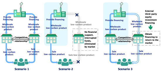
Figure 1.
Structure diagram of LCSC under different financing modes.
For the convenience of modeling, this research makes the following assumptions:
Assumption 1.
Market demand is sensitive to retail prices. Considering consumer preference for low-carbon products, carbon emission reduction expands market demand—higher emission reduction effectiveness increases consumer preference. Thus, the demand expansion from carbon reduction investment is denoted by . Intuitively, higher retail prices decrease market demand, while greater carbon reduction increases it. To ensure economic meaning without loss of generality, market demand is assumed as linear in retail price and carbon reduction investment level . Retailers order low-carbon products based on market demand. According to the research of Yang et al. [9], the inverse demand function for the low-carbon market is
Assumption 2.
This study focuses exclusively on manufacturer carbon emission reduction decisions, where increased manufacturer investment in emission reduction leads to higher costs. The marginal impact of carbon reduction investment on market demand increment exhibits diminishing returns. Consistent with the literature [51,71], the carbon reduction investment cost is defined by a quadratic function , where represents a sufficiently large carbon abatement cost parameter.
Assumption 3.
Following the research of Wang et al. [1], Zheng et al. [8], Zhang et al. [35], and Li et al. [38], we assume a stable and mature LCSC system operating in a single-period scenario. Beyond the manufacturer’s product production costs and carbon reduction investment costs, no additional costs arise between the manufacturer and retailers. Members strictly comply with financing regulations without default events. According to the studies of Cong et al. [72] and Wu et al. [73], the and constraints are assumed.
Assumption 4.
All LCSC members are risk-neutral with complete information symmetry. Manufacturer, retailer, bank, and investment institutions maintain full information transparency [48].
The other symbols involved in the model and their meanings are shown in Table 2.
Table 2.
Description of symbols.
3.2. Benchmark Model
This section elaborates on the core theoretical methodologies underpinning the research to validate model rationality and result reliability. For an LCSC comprising a manufacturer and capital-constrained retailers, drawing on studies of Wang et al. [1], Xia et al. [2], Yang and Zhou [32], and Zhang et al. [35], this paper employs Stackelberg game theory to construct operational decision models under diverse financing modes. A Stackelberg game is a strategic, non-cooperative game theory model featuring a leader and one or more followers. The leader moves first by committing to a strategy (e.g., setting price or quantity), and the followers then optimally respond after observing the leader’s action. This sequential structure grants the leader a first-mover advantage, allowing it to anticipate followers’ reactions and maximize its payoff. Nonlinear optimization theory and backward induction are then applied to derive optimal strategies. In this research, the manufacturer (leader) rationally sets the wholesale price and carbon reduction investment level by anticipating the retailer’s optimal response function, while retailers (followers) determine the retail price of low-carbon products based on these decisions. The strength of these methods lies in game theory’s capacity to analyze interactions among all possible behaviors, yielding equilibrium strategies that enable participants to reach a stable optimal state. Furthermore, the existence and uniqueness of manufacturer–retailer equilibrium strategies are provable via fundamental nonlinear optimization techniques, with solutions obtainable through backward induction—a well-established approach in academia for optimizing structurally simple supply chains, such as in the studies of Yang et al. [9], Wang et al. [22], and Chen et al. [43].
We design a benchmark model serving two primary purposes: First, to establish accurate profit expressions for LCSC members under no capital constraints without financing needs. Second, to provide foundational backward induction methodology for solving subsequent models involving IIF, SIF, and HF. In a manufacturer-led LCSC system, it is assumed that the manufacturer and both retailers are rational decision-makers to maximize their profits. As the leader in the supply chain, the manufacturer incorporates the responses of the two competing retailers into its decision-making process. The two symmetrical retailers are followers and make their judgments by monitoring the manufacturer. Specifically, within the Stackelberg framework, the decision-making sequence among the LCSC participants proceeds as follows: Stage 1: The manufacturer, acting as the Stackelberg leader, announces the wholesale price for low-carbon products and the carbon emission reduction investment level e. Stage 2: Retailer (as the follower) determines the retail price p for low-carbon products based on the manufacturer’s decisions.
Within the LCSC system, the manufacturer is responsible for low-carbon product production and carbon emission reduction technology investments. Consequently, the manufacturer’s profit maximization objective function represents the net profit from product revenue minus carbon reduction investment costs. Product revenue equals unit profit (wholesale price minus production cost) multiplied by the combined order quantities from both retailers. Retailers’ profits are calculated as sales revenue minus ordering costs. The profit functions for the two retailers, manufacturer, and overall LCSC are, respectively, represented as follows (a superscript “*” denotes the optimal equilibrium results, and the same applies hereafter):
First, since , the profit function of retailer is strictly concave with respect to the order quantity . By setting its first derivative equal to zero, the unique optimal order quantity is derived as follows: . Substituting into the manufacturer’s profit function (3), the Hessian matrix of is calculated as
To ensure that attains its maximum at , the Hessian matrix must be negative definite. Given , the function is jointly strictly concave in and when . Solving the first-order conditions simultaneously, we obtain , , and . Substituting into Equation (1), the retail prices are derived as . Further substituting into Equations (2) and (3), the profits of the retailers, the manufacturer, and the whole LCSC are calculated as follows:
4. Pricing and Financing Decision Models for Competing Retailers Under Different Financing Scenarios
In this section, Stackelberg game models are constructed for two competing retailers under three financing scenarios. Using the backward induction method, the optimal equilibrium outcomes are derived, including the manufacturer’s wholesale price, carbon emission reduction investment level, retailers’ optimal retail prices, market order quantities, and profits of all supply chain participants under these scenarios. Subsequently, the contract coordination conditions for forming a supply chain alliance between the manufacturer and one retailer are analyzed. Finally, the conditions under which the manufacturer permits the other retailer to re-enter the market and engage in competition are examined.
4.1. Scenario Where Manufacturer Provides Financing to Both Retailers Simultaneously (IIF)
In this financing scenario, both retailers engage in free competition, face capital constraints, and lack funds for product ordering. The manufacturer provides financing to both retailers through a delayed-payment trade credit model. As the leader of the LCSC system, the manufacturer is responsible for producing low-carbon products and first determines the wholesale price and carbon emission reduction investment level . Acting as followers, the two retailers order low-carbon products and based on and then sell them to consumers at retail prices and , respectively, to earn price differences and generate revenue. However, both retailers order products on credit and compete in quantities. At the end of the operating period, the retailers repay the manufacturer the principal and interest at the financing interest rate . The manufacturer’s profit includes the principal and interest received from the retailers minus the production cost of the low-carbon products, the opportunity cost of the capital used for production, and the carbon emission reduction investment cost. Therefore, the profit functions for the retailers, manufacturer, and the entire LCSC are defined as follows:
Proposition 1.
When the manufacturer provides financing to both competing retailers, the manufacturer’s optimal wholesale price, optimal carbon emission reduction investment level, retailers’ optimal market order quantities, optimal retail prices, and maximum profits for the retailers, manufacturer, and whole LCSC are given by the first column of Table 3.
Table 3.
Equilibrium results under different financing models.
Proof of Proposition 1.
First, since , the profit function of retailer is strictly concave with respect to the order quantity . By setting its first derivative equal to zero, the unique optimal order quantity is derived as , . Substituting into the manufacturer’s profit function (5), the Hessian matrix of is calculated as . To ensure that attains its maximum at , the Hessian matrix must be negative definite. Given , the function is jointly strictly concave in and when . Solving the system of first-order conditions , we obtain , , and . Substituting these optimal equilibrium results into Equation (1), the retail prices are derived as . Finally, combining Equations (4) and (6), the profits of the retailers, manufacturer, and the entire LCSC are calculated as , , . □
Property 1.
, , , , , , .
Proof of Property 1.
, , , , , , . □
According to Property 1, in a competitive environment with two retailers, when the manufacturer provides financing to both capital-constrained retailers, their symmetry results in identical wholesale prices set by the manufacturer. Consequently, the retailers maintain equal order quantities, retail prices, and profits. As competition intensifies between the two retailers, the manufacturer’s wholesale price, carbon emission reduction investment level, retailers’ order quantities, retail prices, as well as profits of both LCSC members and the overall system exhibit marginally decreasing trends. From the perspectives of supply chain game theory and marginal economics, intensified competition reduces demand price elasticity . Simultaneously, marginal order quantities and their rates of change turn negative. The sales-stimulating effect of retail price reductions strengthens progressively, while heightened competition shifts retailers’ marginal profit curves downward. Consequently, the manufacturer is compelled to lower wholesale prices to sustain sales volume. When competition intensifies, the manufacturer may delay upgrading low-carbon equipment because the marginal returns from market orders cannot offset the marginal costs of emission reduction, leading to diminishing marginal profits. To counteract this deteriorating dynamic, the manufacturer—as the leader of the LCSC system—may form a supply chain alliance with one retailer to maximize self-interest while ensuring product carbon compliance. This excludes the other retailer from financing access, exposing it to funding discontinuity risks and potential market exit.
Property 2.
(1) , , , , , , . (2) , , , , , , .
Proof of Property 2.
, , . , , , , . □
Property 2 indicates that when the manufacturer provides financing to both competing retailers, the wholesale price inversely correlates with the financing interest rate but positively correlates with the bank credit interest rate. This can be explained as follows: when the opportunity cost of production rises, the manufacturer raises the wholesale price to offset profit losses, indirectly prompting retailers to increase their retail prices. The carbon emission reduction investment level, market order quantities of both retailers, retail prices, and profits of LCSC members are unaffected by the financing interest rate but are influenced by the bank credit interest rate. Specifically, an increase in the bank credit interest rate reduces the manufacturer’s carbon reduction investments, retailers’ order quantities, and supply chain participants’ profits. High opportunity costs weaken the manufacturer’s motivation to reduce carbon emissions, leading to a sluggish low-carbon market and negatively impacting both individual supply chain members and overall profits.
4.2. Scenario Where Manufacturer Provides Financing to Single Retailer (SIF)
Assuming the manufacturer aims to maximize its profits by forming a supply chain alliance with one retailer, it offers trade credit only to retailer , while the other retailer loses access to financing, faces funding disruption, and is eliminated from the market. In this scenario, the LCSC system becomes a game between the manufacturer and a single capital-constrained retailer, eliminating competition between the two retailers. The inverse demand function and the profit functions for the remaining retailer and the manufacturer are defined as:
Similarly to the derivation process in Proposition 1, backward induction is applied here, and the detailed steps are omitted for brevity.
When the manufacturer provides financing to a single retailer, the manufacturer’s optimal wholesale price, optimal carbon emission reduction investment level, retailer ’s optimal market order quantity, optimal retail price, and maximum profits for the manufacturer, retailer and entire LCSC are given by , , , , , , and .
Conclusion 1.
Compared to the scenario where the manufacturer provides financing to both capital-constrained retailers simultaneously, ,
, , and should be satisfied.
Proof of Conclusion 1.
, , , . □
Conclusion 1 demonstrates that under wholesale-price contracts, the manufacturer rejects forming an alliance with retailer and refuses to provide IIF. This occurs because alliances erode manufacturer profit under such contracts, resulting in lower wholesale prices, reduced carbon emission reduction investment level, diminished market order quantities from retailers, and decreased manufacturer profit compared to Scenario 1.
To ensure economically meaningful equilibrium outcomes in model construction, this study assumes all members are risk-neutral and maintain complete information symmetry—where the manufacturer, retailers, banks, and investment institutions share full transparency [9,74]. Furthermore, under compliant financing and operational practices, we assume zero default or bankruptcy risks among supply chain members [48]. Meanwhile, this study initially proposes a wholesale-price contract model, which contradicts manufacturer alliance-formation incentives. To eliminate double marginalization, we design a revenue-sharing contract that achieves perfect coordination in the LCSC. This mechanism safeguards alliance members’ profits while motivating the manufacturer and retailer to forge strategic alliances, thereby securing monopoly market advantages.
First, the optimal equilibrium solution is calculated when the manufacturer and retailer engage in centralized decision-making. The total profit function of the LCSC is
It is straightforward to verify , , indicating that is jointly concave in and . Solving the system of first-order derivative equations yields
Following the revenue-sharing principle, retailer shares a proportion of its sales revenue with the manufacturer, while the manufacturer retains . The profit functions for retailer and the manufacturer are then defined as
Proposition 2.
Under the revenue-sharing contract, the manufacturer’s redefined wholesale price is , and when
, the contract achieves perfect coordination and is acceptable to all LCSC members. The equilibrium results are also shown in the second column of Table 3.
Proof of Proposition 2.
Using the backward induction method, we derive . To achieve perfect coordination of the LCSC, ensuring that the total profit under the revenue-sharing contract equals that under centralized decision-making, the conditions and need to be satisfied. Consequently, we obtain the redefined wholesale price under the perfect coordination contract as , the carbon emission reduction investment level as , the market order quantity as , and the retailer’s selling price as . Substituting the above optimal equilibrium results into Equations (11) and (12), we obtain and . The total profit of the LCSC is . To ensure that both the manufacturer and retailer accept this coordination contract, the profits of all participants in the LCSC must not be lower than their respective profits under decentralized decision-making. The revenue-sharing ratio must satisfy . □
Property 3.
, , , , , , .
Proof of Property 3.
, , , , , , . □
Property 3 indicates that when the manufacturer provides financing exclusively to a single capital-constrained retailer and forms a supply chain alliance, the manufacturer’s wholesale price and the retailer’s retail price increase as the bank credit interest rate rises. Conversely, the carbon emission reduction investment level, the retailer’s market order quantity, and the profits of both supply chain participants (as well as the overall supply chain) decrease with a higher bank credit interest rates. This can be explained as follows: An increase in the bank credit interest rate raises the manufacturer’s opportunity cost of production, prompting the manufacturer to increase the wholesale price to offset potential profit losses. This indirectly drives up the retail price, which may weaken demand for low-carbon products due to market supply-demand dynamics, thereby reducing market order quantities and discouraging the manufacturer’s carbon reduction investments. The inequality holds, indicating that the rate of decline in market order quantity exceeds the rate of increase in retail prices. This phenomenon highlights the more significant impact of reduced market order quantity, leading to profit declines for all supply chain participants and the overall supply chain. Additionally, it is observed that only the wholesale price decreases when the manufacturer’s financing interest rate rises, while other variables and profits remain unaffected.
Conclusion 2.
When comparing Financing Scenario 2 to Scenario 1, the relationships ,
, and hold.
Proof of Conclusion 2.
, , . □
Conclusion 2 demonstrates that when the manufacturer and retailer adopt a coordinated contract to form a supply chain alliance (compared to the scenario where the manufacturer finances two competing retailers), the low-carbon product market exhibits broader prospects. Specifically, market order quantity increases, the manufacturer’s carbon reduction investments are enhanced, products become lower-carbon, and reduced retail prices make them more appealing to consumers. The willingness of the manufacturer and retailer to form an alliance depends on the competition intensity between the retailers. As shown in Property 1, higher competition lowers profits for supply chain participants, prompting the manufacturer to consider allying with one retailer. Conclusion 3 defines the contractual conditions for such a supply chain alliance.
Conclusion 3.
Let . When
, neither the manufacturer nor retailer is willing to form an LCSC alliance. When and , both the manufacturer and retailer agree to form an alliance. If , retailer rejects the alliance. When , the manufacturer becomes unwilling to collaborate.
Proof of Conclusion 3.
, , let , according to the properties of the quadratic function, when , holds. It follows that . □
Combined with Property 1, the higher the competition intensity between the two retailers, the more it negatively impacts the profits of all supply chain participants. According to Conclusion 3, for the manufacturer and one retailer to agree to form a supply chain alliance, specific constraints must be met: and . Only under these conditions can the double marginalization effect be mitigated, ensuring higher profits for the alliance compared to Scenario 1. Otherwise, neither party is willing to collaborate. This aligns with findings from Yang et al. [9], who studied three financing scenarios and confirmed that supply chain alliances benefit all participants when suppliers partner with a retailer [48]. We further incorporate the influence of consumer low-carbon preferences. By analyzing low-carbon product market demand under manufacturer carbon reduction investments, we address financing challenges for two capital-constrained retailers. Similarly, when competition between retailers intensifies, the manufacturer and one retailer will only form an alliance if the profit-sharing ratio lies within the Pareto zone. Otherwise, at least one party rejects collaboration. If an alliance is formed, the excluded retailer (without financial support) risks being squeezed out of the low-carbon market, and facing bankruptcy. To sustain competitiveness and re-enter the market, the excluded retailer may adopt HF—combining bank credit with equity financing from third-party investors—to strengthen its position in the low-carbon market.
4.3. Scenarios Where Individual Retailer Returns to Market with Blended Financing (HF)
When the low-carbon manufacturer forms a supply chain alliance with retailer , the other retailer is excluded from the market due to a lack of financial support. To sustain operations, retailer relies on HF channels to secure funding and maintain cash flow. It is assumed that retailer obtains the required funds through equity financing from a third-party investor, agreeing to distribute a proportional dividend to the investor. For model simplicity, the equity financing ratio is assumed to be equal to the dividend distribution ratio. The remaining portion of the funding needs is met via bank credit, requiring interest payments and incurring financing costs. Under these circumstances, the manufacturer continues to provide financing to retailer , while retailer utilizes HF to order low-carbon products and compete with retailer . The manufacturer sets identical wholesale prices for both retailers. The inverse demand functions for the two retailers are
At this point, the profit functions for the two retailers and the manufacturer are expressed as follows:
Proposition 3.
Under competitive conditions, when the excluded retailer re-enters the market via HF, the manufacturer’s optimal wholesale price, the optimal carbon emission reduction investment level, the two retailers’ optimal market order quantities, the optimal retail prices, and their maximum profits are shown in the third column of Table 3.
Property 4.
When the excluded retailer re-enters the market using HF, the manufacturer’s wholesale price, the carbon emission reduction investment level, and the two retailers’ market order quantities and retail prices exhibit the following relationships with respect to the equity financing ratio: , , , , , .
Proof of Property 4.
, where . Differentiating V with respect to , , which implies and . To simplify calculations, let . Then, . The sign of depends on : , thus, . Similarly, it can be proven that , , . □
Property 4 demonstrates that when the other retailer re-enters market competition utilizing HF, increasing the equity financing ratio enables the retailer to secure capital support from third-party investment institutions, thereby enhancing its competitive advantage. For instance, Blue Valley Smart Energy Co., Ltd. obtained over RMB 300 million in financing from four investment institutions including BAIC New Energy and SK New Energy. These funds were allocated to market expansion and innovation of eco-friendly energy products, strengthening core competitiveness. From the integrated perspectives of supply chain game theory and marginal economics, an increase in the equity financing ratio induces a negative marginal order quantity for retailer , positive marginal order quantity for retailer , and positive marginal carbon reduction effort for manufacturer , indicating that equity-financed retailer escalates low-carbon product procurement while simultaneously eroding ’s competitive position. To maximize self-interest, the manufacturer elevates the wholesale prices while intensifying carbon reduction efforts—emitting positive signals to stimulate increased low-carbon product orders from the retailer and strategically favoring ’s market re-entry. Simultaneously, both retailers exhibit positive marginal retail prices, confirming that their selling prices rise with increasing equity financing ratios.
Conclusion 4.
When a previously excluded retailer re-enters the market through HF, the equity financing ratio impacts supply chain profits as follows: the profit of retailer decreases as increases, while retailer ’s profit increases with only if specific conditions are met; otherwise, it declines. The manufacturer permits ’s re-entry into the market if and only if . If this profitability condition is not satisfied, the manufacturer prioritizes forming a supply chain alliance with the retailer over allowing to re-engage in competition.
Proof of Conclusion 4.
The partial derivative of retailer ’s profit with respect to the equity financing ratio is . According to Property 4, . This shows that the profit of retailer is monotonically decreasing with respect to the equity financing ratio , meaning it decreases as increases. The partial derivative of retailer ’s profit with respect to the equity financing ratio is . When the equity financing ratio satisfies the inequality , the profit of retailer increases as increases. Otherwise, it decreases with increases in . Given the computational complexity of comparing the manufacturer’s profits in Scenario 2 and Scenario 3, this study employs numerical simulations to identify the valid range of the equity financing ratio under which the manufacturer allows retailer to re-enter the market. This approach verifies the model’s rationality and the conclusions’ validity. □
Conclusion 4 indicates that retailer , by re-entering the market through an HF model combining external bank credit and equity financing, gains a competitive advantage over retailer in ordering low-carbon products. This advantage becomes more pronounced as the equity financing ratio increases, but there exists an optimal equity financing ratio that maximizes ’s profit. Equity financing serves as an effective solution to alleviate the funding constraints of capital-constrained retailers, enhancing market competitiveness and rapidly expanding ’s operational scale, thereby weakening its rival’s competitiveness or even driving the competitor out of the market. As the leader of the supply chain, the manufacturer permits to re-enter the market only if its profit under this scenario exceeds the profit from forming an alliance with retailer in Scenario 2. Otherwise, ’s re-entry is disallowed.
5. Numerical Simulation
In this section, we focus on analyzing the magnitude of impact and evolution patterns of key parameters—including competition intensity, financing interest rates, and equity financing proportions—on decision variables and profits across IIF, SIF, and HF. This is achieved by computing the first-order derivatives of these parameters. Parameter configurations must satisfy the theoretical model’s assumptions; thus, the values used in the simulations are specified in Table 3. The specific simulation results are presented in Table 4 and Table 5 and Figure 2, Figure 3, Figure 4, Figure 5, Figure 6, Figure 7, Figure 8, Figure 9 and Figure 10.
Table 4.
Relevant parameter settings in simulation.
Table 5.
The change in decision variables and profits with the bank interest rate after an alliance is formed.
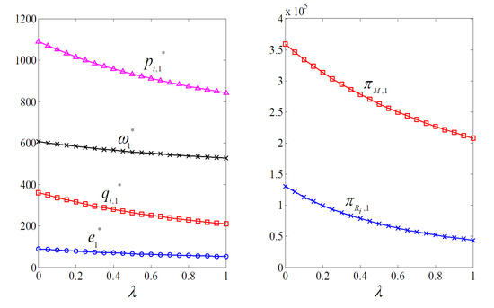
Figure 2.
The impact of competition intensity λ on equilibrium results under Scenario 1.
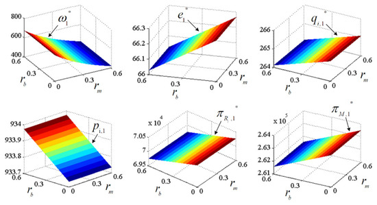
Figure 3.
The impact of and on equilibrium results under Scenario 1.
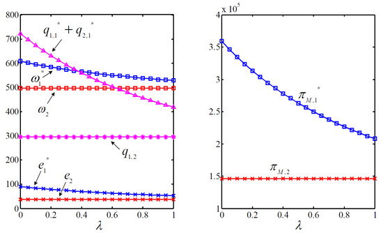
Figure 4.
Comparison of Scenario 1 and Scenario 2 without alliance.
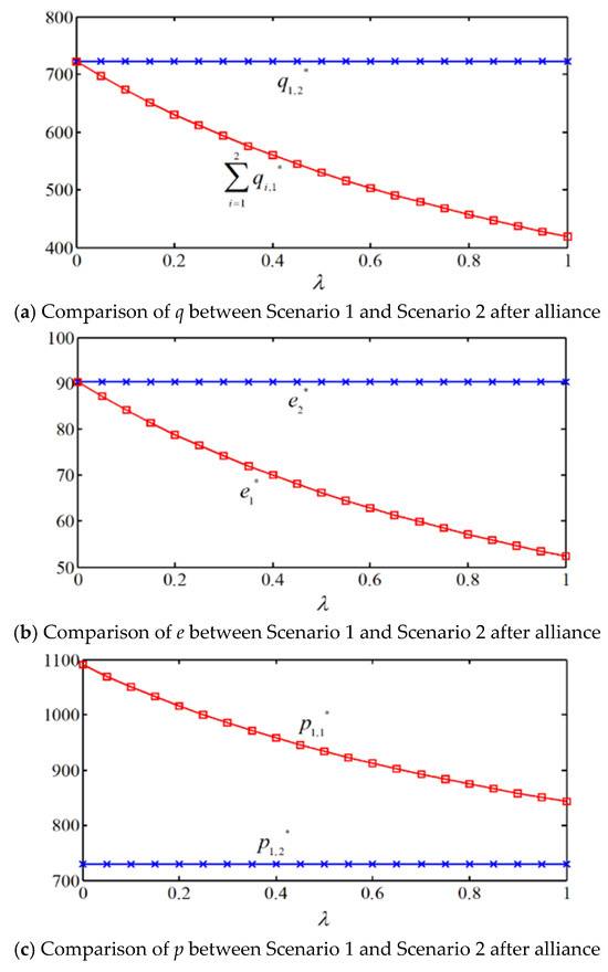
Figure 5.
Comparison of q, e, and p between Scenario 1 and Scenario 2 after alliance.
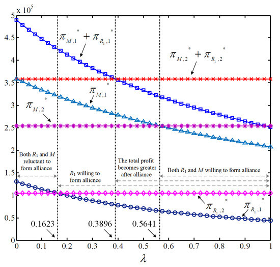
Figure 6.
Analysis of manufacturer–retailer alliance conditions.
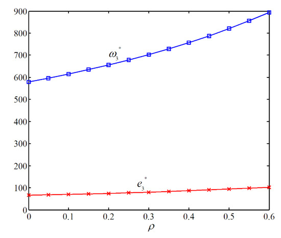
Figure 7.
The change trends for and with .
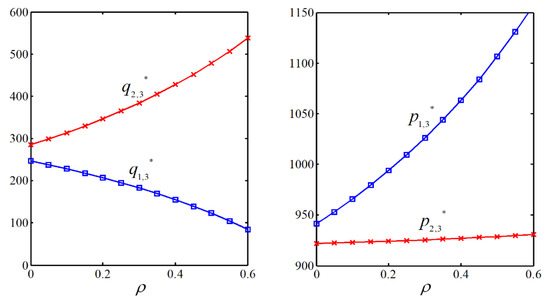
Figure 8.
The change trends for and with ().
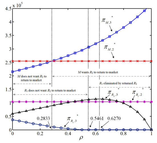
Figure 9.
An analysis of the conditions under which the manufacturer allows retailer to return to the market.
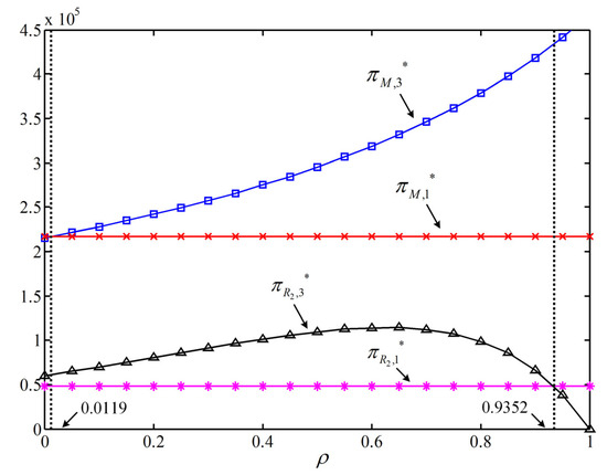
Figure 10.
The profits of the manufacturer and retailer with and without equity financing.
5.1. Manufacturer Provides Financing to Both Retailers Simultaneously
5.1.1. Analysis of Impact of Competition Intensity
From Figure 2, it is observed that under Scenario 1 (where the manufacturer provides financing to both retailers simultaneously), the wholesale prices set by the manufacturer for the two retailers are equal. Due to the symmetry between the retailers, their market order quantities and retail prices are also identical. As the competition intensity increases, both the manufacturer’s wholesale price and carbon emission reduction investment level exhibit a declining trend. Meanwhile, the competitive behavior between the two retailers leads to a decline in market order quantities, with a faster rate of decrease compared to the wholesale price. Consequently, the manufacturer’s profit experiences a more pronounced reduction. As competition intensity increases, both the retail prices and market order quantities (demand) of the two retailers decrease, resulting in a decline in the profits of both retailers.
Furthermore, according to Figure 2, as competition intensity increases, retailer order quantity and carbon emission reduction investment level both decrease significantly: drops from 361.24 to 209.14, while declines from 90.31 to 52.28—both reductions reaching 42.11%. The equilibrium outcomes for retail price and wholesale price decrease from 1090.3 to 843.1 and 607.56 to 528.34, representing reductions of 22.67% and 13.04%, respectively. Consequently, profits for both retailers and the manufacturer decline: retailers’ profits fall from 130,490 to 43,740 (66.48% decrease) and manufacturer profits decrease from 358,850 to 207,760 (42.10% decrease). Furthermore, we analyze the trends of manufacturer’s and retailers’ profits concerning . When , the rates of change in profits for manufacturer and retailers and are and with the corresponding profit values . The sensitivity of profit changes to is quantified as and , which indicates differential sensitivity to competition intensity: Increased competition more significantly impacts retailers’ profits. This occurs because heightened competition reduces retail prices and order quantities, with retail prices declining faster than wholesale prices. Consequently, competition intensity exerts a more pronounced effect on retailers’ profits.
5.1.2. Analysis of Impact of and
From Figure 3, it is observed that under Scenario 1, the manufacturer’s financing interest rate and the bank credit interest rate jointly influence the decision variables and profits of the supply chain participants. The manufacturer’s wholesale price is jointly affected by and . The wholesale price decreases as increases but increases with a rise in . This is because represents the interest rate set by the manufacturer for charging the retailers. When increases, the financing costs borne by the retailers rise, forcing the manufacturer to lower the wholesale price to incentivize the retailers to order low-carbon products. Conversely, when increases, the manufacturer’s opportunity cost of production increases, leading the manufacturer to raise the wholesale price to offset the additional costs. Other decision variables and the profits of supply chain participants remain unaffected by . However, when increases, the manufacturer’s carbon emission reduction investment level, market order quantities, and overall supply chain profits decrease, while the retail prices of both retailers increase. This phenomenon indicates that the conclusions and properties derived from the IIF equilibrium between a single manufacturer and a single capital-constrained retailer also apply to the scenario where a single manufacturer provides IIF to two competing and capital-constrained retailers simultaneously.
5.2. Manufacturer Provides Financing to Single Retailer Only
5.2.1. The Manufacturer Provides Financing to a Single Retailer Without Forming an Alliance
When the manufacturer provides financing only to retailer (Scenario 2), retailer , unable to obtain financing support, is likely to exit the market. Under the wholesale-price contract, the optimal equilibrium results for the decision variables and the manufacturer’s profit are solved as shown in Figure 4.
Compared to Scenario 1, both the decision variables and the manufacturer’s profit decline. Since the wholesale price, carbon emission reduction investment level, market order quantities, and manufacturer’s profit are all reduced, the manufacturer will not form a supply chain alliance with retailer under the wholesale-price contract. To avoid double marginalization, the manufacturer and retailer must revise the contract terms by designing a revenue-sharing contract to achieve perfect coordination in the LCSC. The designed revenue-sharing ratio must fall within a reasonable range to ensure that the profits of both retailer and the manufacturer exceed their pre-coordination levels. Under these conditions, the whole LCSC profit is maximized, incentivizing the manufacturer and retailer to form a monopolistic alliance, while capital-constrained retailer is eliminated from the market.
5.2.2. The Manufacturer Provides Financing to a Single Retailer and Forms an Alliance
When the manufacturer provides financing only to retailer (Scenario 2) and forms a supply chain alliance, a revenue-sharing ratio of is set. Through the designed revenue-sharing contract, perfect coordination among supply chain participants is achieved. By sharing a portion of the retailer’s revenue, the manufacturer sets a significantly lower wholesale price; otherwise, retailer would refuse to form the alliance. However, as the bank credit interest rate increases, the manufacturer’s opportunity cost of production rises, leading to an increase in the wholesale price, as shown in Table 5. High bank credit opportunity costs reduce retailer ’s profit. When , the rates of change in retailer ’s order quantity and retail price are and , respectively, indicating that the decline in order quantity outpaces the rise in retail price. As the bank credit interest rate increases, the growing opportunity cost of production weakens the manufacturer’s motivation for carbon emission reduction, resulting in a decline in carbon reduction investment levels. The higher retail prices also dampen consumer demand, negatively impacting the profits of the participants and the whole LCSC.
5.2.3. Comparison of q, e, and p Between Scenario 2 and Scenario 1 After Alliance Formation
A comparison of the impacts on the market, environment, and consumers before and after the manufacturer forms a supply chain alliance with retailer (i.e., between Scenario 1 and Scenario 2) is illustrated in Figure 5. Based on Property 1 and Figure 2, this figure reveals that under Scenario 1 (manufacturer provides financing to both retailers), as the competition intensity increases, the carbon emission reduction investment level, market order quantities, and retail prices all exhibit declining trends, leading to reduced profits for supply chain participants. In contrast, under Scenario 2 (manufacturer finances only one retailer), a revenue-sharing contract coordination mechanism can incentivize the manufacturer and retailer to form an alliance.
Further analysis shows that when the manufacturer and retailer agree to form an alliance, the revenue-sharing ratio must fall within the interval to ensure mutual benefits. Post-alliance, market demand expands, order quantities increase, the manufacturer’s motivation for carbon reduction strengthens, and retail prices become more consumer-friendly. Numerical simulations demonstrate that at , , and , the differences before and after alliance formation are , , and . This indicates that after forming the alliance, market order quantities increase by 219.35, carbon emission reduction investment rise by 27.42, and retail prices decrease by 365.59.
In Scenario 2, the alliance between the manufacturer and retailer creates a monopoly, yielding favorable market outcomes. The alliance incentivizes the manufacturer to enhance carbon reduction efforts, improving product competitiveness. The low-carbon attributes and consumer-friendly prices stimulate purchasing demand, increasing market demand for low-carbon products. The expanded demand allows retailer to dominate the low-carbon market, while retailer is eliminated from competition.
5.2.4. Analysis of Alliance Willingness Between Manufacturer and Retailer
First, the feasible range for the manufacturer and retailer to form an alliance was analyzed. Based on the assigned values of and , when the revenue-sharing ratio lies in the interval , retailer ’s profit decreases post-alliance, making the retailer unwilling to form the alliance. When falls within , the manufacturer’s profit decreases, leading the manufacturer to reject the alliance. Only when is within do both the manufacturer and retailer achieve higher profits post-alliance. Thus, is a necessary condition for perfect coordination.
Assuming , the impact of competition intensity on alliance willingness is analyzed in Figure 6. When , the manufacturer’s profit and retailer ’s profit , so neither party is willing to form an alliance. As competition intensity increases to , the manufacturer’s profit remains , while retailer ’s profit becomes and the manufacturer rejects the alliance. However, the total supply chain profit declines; i.e., .
When the competition intensity , the total supply chain profit satisfies . However, the manufacturer’s profit remains lower than pre-alliance levels, i.e., , while retailer ’s profit satisfies . Under these conditions, the manufacturer remains unwilling to form an alliance, whereas retailer is willing. When falls within , the manufacturer’s profit becomes and retailer ’s profit satisfies . The total supply chain profit meets . In this case, both members are willing to form an alliance, and the total post-alliance profit exceeds that of Scenario 1. Furthermore, post-alliance market order quantities and carbon reduction levels consistently surpass those in Scenario 1, while retail prices remain lower. This phenomenon indicates that the alliance fosters the healthy development of the LCSC system.
5.3. Single Retailer Re-Enters Market with HF
5.3.1. Impact Analysis of Equity Financing Ratio
When the low-carbon manufacturer chooses to form a supply chain alliance with retailer , the other retailer, , unable to obtain financial support from the manufacturer, faces the risk of market elimination. To sustain operations, retailer secures funding through HF channels to ensure normal cash flow. Assuming retailer adopts external HF—obtaining a portion of funds from third-party equity investors and the remainder from bank credit—the equity financing ratio is set equal to the equity dividend ratio for model simplification. With competition intensity , the trends of key variables with respect to are analyzed, as shown in Figure 7 and Figure 8.
From Figure 7 and Figure 8, it can be observed that when retailer re-enters the market with HF to participate in competition, the manufacturer’s optimal wholesale price, the optimal carbon emission reduction investment level, retailer ’s order quantity, and the retail prices of both retailers all increase with the equity financing ratio . Conversely, retailer ’s order quantity decreases as increases. This phenomenon indicates that when retailer re-enters the market with external financial support, a higher equity financing ratio enhances ’s core competitiveness, gradually strengthening its competitive advantage within the supply chain. Retailer , supported by increased third-party equity financing, expands its product orders to capture the low-carbon retail market. To maximize its profit, the manufacturer raises the wholesale price and intensifies carbon reduction efforts, signaling support for ’s increased low-carbon product orders. Under these conditions, the manufacturer strongly prefers retailer ’s re-entry into the market.
Meanwhile, the optimal retail prices of both retailers increase with . As shown in Figure 8, retailer ’s optimal retail price consistently remains lower than retailer ’s price, with a smoother variation trend as changes. This suggests that retailer , upon re-entering the market, exhibits stronger consumer market affinity. After ’s return to the market, the combined effects of higher wholesale prices and declining consumer purchasing desire significantly weaken retailer ’s market competitiveness, creating a risk that may be eliminated by .
5.3.2. The Conditions Under Which the Manufacturer Allows Retailer to Return to the Market
As the dominant player in the supply chain, the manufacturer has the power to decide whether to allow retailers to return to the market to compete. We analyze the impact of the equity financing ratio on the profits of the supply chain participants in Scenarios 2 and 3 when retailer uses blended financing to return to the market to compete, as shown in Figure 9.
According to Figure 9, if , indicating a high market competition intensity. Under this condition, the manufacturer is willing to form a supply chain alliance with the retailer . When retailer re-enters the market to participate in competition with financial support from third-party institutions, the manufacturer’s profit increases with the equity financing ratio , while the retailer ’s profit gradually decreases as increases. Retailer ’s profit increases with only when the equity financing ratio meets certain conditions; otherwise, it decreases with . Additionally, there exists an optimal value that maximizes ’s profit.
To clearly analyze the conditions under which the eliminated retailer can re-enter the market to compete and the impact of ’s return on the profit of the allied retailer , we conducted a comparative analysis of two scenarios. First, comparing the profits of the manufacturer and the allied retailer between Scenario 2 and Scenario 3 reveals distinct patterns. When the equity financing ratio lies within the interval , the manufacturer’s profit satisfies and retailer ’s profit satisfies , leading both the manufacturer and retailer to oppose retailer ’s re-entry into the market for competition. When falls within , the manufacturer’s profit becomes , while retailer ’s profit remains . In this case, the manufacturer supports retailer ’s re-entry, but retailer opposes it. As continues to increase into the interval , the manufacturer’s profit still satisfies , and the manufacturer continues to support retailer ’s re-entry into market. And more, as increases, ’s profit first increases and then decreases, reaching its maximum value of 114,280 at . This represents a 91.55% increase compared to its value at (where ). However, retailer ’s profit drops to =0, resulting in ’s elimination from the market due to an inability to generate profit. Furthermore, comparing profits between Scenarios 1 and 3 for the manufacturer and retailer (as shown in Figure 10): When , while . As increases, gradually rises. At , . When , . During this process, it can be observed that first increases then decreases, reaching at .
Based on the theoretical analysis and numerical simulations above, this study contextualizes Procter & Gamble’s (P&G) real-world commitment to integrating sustainable low-carbon development principles into product innovation, actively reducing corporate and product carbon footprints, and adopting more circular methods in its supply chain to achieve a reduction in carbon emissions through improved energy efficiency. Faced with two capital-constrained and competing retail stores—Hualian Daoli Store and Hualian Daowai Store—P&G could initially provide delayed payment trade credit to both retailers. However, P&G would observe that as the competition between retailers intensified, its own profits and the overall supply chain profits decline instead of increasing. Consequently, P&G would consider altering its financing strategy by providing delayed payment trade credit exclusively to the Hualian Daoli Store and designing a revenue-sharing contract to form a supply chain alliance. Meanwhile, Hualian Daowai Store could re-enter the market to compete by securing financing through bank loans and third-party equity investments.
6. Discussion and Management Recommendations
6.1. Results and Discussion
Our research reveals that three financing strategies (IIF, SIF, and HF) significantly impact LCSC operations. First, intensified competition constrains order quantities for capital-constrained retailers and impedes manufacturer carbon emission reduction efforts. This finding aligns with the conclusion of Yang et al. [74]. Extending beyond their work, we further examine financing models, clarifying how these three modes influence system operations and profit distribution. The study demonstrates that IIF proves disadvantageous: under this model, heightened retailer competition triggers low-carbon product market depression, directly undermining supply chain members’ profits and discouraging manufacturers’ emission reduction initiatives. Second, building upon the research of Yang et al. [9], we extend the analysis beyond IIF by introducing SIF and IF models to further examine their systemic impacts. The study reveals that under SIF, the non-allied retailer exits the market due to capital constraints, while the profits for the allied retailer and manufacturer do not uniformly increase—their outcomes being contingent on competition intensity and alliance contract selection. Conversely, IF reignites competition: it enhances the non-allied retailer’s profit but diminishes the allied retailer’ returns. Notably, when the equity financing ratio exceeds certain thresholds, the allied retailer faces market elimination through crowding-out effects. Finally, a comparative analysis of the three financing models reveals that, from a system-wide profitability perspective, IIF is preferable when financing interest rates are low due to reduced financing costs. Regarding carbon emission reduction performance, SIF emerges as the dominant strategy. For retailers, optimal selection depends critically on financing rates and competition intensity: IIF dominates under low competition intensity, while HF is preferred by retailers otherwise.
In summary, across all three financing models, heightened competition intensity consistently undermines system operations—manifested through reduced product market prices, diminished manufacturer carbon reduction efforts, and decreased overall profitability. When competition intensity remains fixed, under IIF, wholesale prices, order quantities, and participant profitability do not uniformly increase but depend on loan interest rates. Under SIF, the non-allied retailer faces capital chain disruptions and market elimination due to funding shortages. While under HF, the non-allied retailer re-enters the market through external financing, when the equity financing ratio exceeds critical thresholds, this reduces the allied retailer’s profit and may even trigger its market elimination via crowding-out effects.
6.2. Managerial Recommendations
6.2.1. Government
Government top-level planning plays a crucial role in the operation of the supply chain system, particularly for LCSC systems. Therefore, based on the above discussion, this paper recommends that the government establish a scientific subsidy policy system tailored to its fiscal capabilities.
First, it is recommended that the government standardize market competition order. Since intensified competition among retailers continuously damages product order volumes, weakens manufacturers’ carbon emission reduction efforts, and erodes the overall profitability of the LCSC, ultimately undermining system sustainability, the government should regulate market competition orders. This includes establishing a dynamic monitoring and early warning mechanism for retailer competition intensity, and mandating differentiated product entry policies along with long-term stability agreements among supply chain members. These agreements should incorporate minimum order quantities and emission reduction investment sharing to disperse excessive competitive pressure and align the sustainable interests of all parties.
Second, it is recommended that the government optimize financing policy design and ensure financing fairness. Since, under IIF, an increase in bank credit interest rates significantly reduces the manufacturer’s emission reduction investment, retailers’ order quantities, and the profits of all participants, while financing interest rates only affect wholesale prices, the government should prioritize supporting the IIF model. For instance, the government could establish a “Green Supply Chain Loan Fund” to subsidize bank credit interest rates (e.g., providing interest rate subsidies on amounts exceeding the benchmark rate) and implement fiscal tools such as tiered value-added tax deductions. These measures aim to stabilize emission reduction investments and supply chain operations, shielding them from the negative impacts of interest rate fluctuations, particularly those related to bank credit rates. Furthermore, under SIF, the non-supported retailer faces market elimination, and this model underperforms overall compared to IIF. Since the feasibility of revenue-sharing-contract alliances heavily depends on profit distribution and competition intensity—making them prone to market imbalance—it is recommended that the government mandate non-discriminatory financing access as a compulsory prerequisite for enterprises to obtain public resources (e.g., subsidies, tax incentives). The government should strictly restrict and regulate SIF (especially wholesale-price-contract alliances), establish profit distribution intervals and competition intensity red lines for revenue-sharing contracts, and implement early-warning systems for retailer exit alongside rapid anti-monopoly response mechanisms. These measures aim to uphold fair market competition and ensure the viability of small and medium-sized retailers.
Third, it is recommended that the government guide the rational development of HF. Under this model, the non-allied retailer re-entering the market through external equity financing—particularly when the equity financing ratio exceeds a critical threshold—can disrupt existing alliances, intensify competition, and potentially replace alliance participants via the “market crowding effect”, thereby harming the interests of the allied retailer. Therefore, the government should establish constraints on equity-financed re-entry, such as requiring reporting for ratios exceeding specified levels and prohibiting short-term price wars post-re-entry, imposing high-competition adjustment levies on enterprises triggering market crowding effects, and creating an Alliance Stability Guarantee Fund to provide compensation and transitional financing support to affected alliance members—ultimately balancing the vitality of new entrants with the stability of established alliances.
Fourth, it is recommended that the government strengthen LCSC infrastructure development. Due to the lack of effective monitoring mechanisms and diversified financing channels, entire LCSCs face multidimensional risks spanning competition, financing, and emission reduction. Therefore, the government should deepen the construction of an integrated LCSC digital supervision platform to enable real-time monitoring and intelligent early warnings for carbon footprints, order fluctuations, financing transmission, and competition intensity. Concurrently, it should promote financial innovations such as the securitization of carbon reduction performance (e.g., issuing carbon revenue bonds), thereby transforming emission reduction investments into tradable assets. These initiatives will broaden access to low-cost, low-interest-rate-sensitive financing channels for supply chain members while enhancing the system’s overall resilience and risk management capacity.
Finally, governments should innovate policy tools to alleviate bottlenecks in low-carbon transition amid fiscal constraints. To ensure the sustainable development of CLSCs, a dual strategy is recommended: leveraging policy instruments to mobilize private capital while stimulating inherent market vitality. Specifically, we recommend (1) establishing a government-guaranteed Low-Carbon Transition Risk Compensation Fund (with limited public exposure to subordinated risks) to incentivize financial institutions like banks in expanding green credit to LCSC members—particularly small and medium retailers—(2) deepening emissions trading market reforms, by permitting manufacturers to use verified carbon reductions for collateralized financing or direct trading, while pioneering a “Securitization Model for Projected Carbon Reduction Revenues” to convert future decarbonization income into immediate low-cost financing capacity. These measures effectively overcome funding barriers with minimal fiscal input, thereby sustaining momentum for emission reduction investments and supply chain decarbonization. Concurrently, governments should enhance the development and open sharing of public LCSC digital supervision platforms to reduce corporate compliance costs and financing information gaps, ultimately boosting systemic resource efficiency.
6.2.2. LCSC System and Members
First, from the perspective of the LCSC system, alliance stability largely depends on the profit-sharing ratio and competition intensity. Consequently, all supply chain members should establish transparent contract governance mechanisms with real-time sales and emissions data sharing. Notably, decentralized competition and financing models exacerbate internal friction, weaken carbon emission reduction incentives, diminish overall profits, and destabilize the system through market crowding effects triggered by HF. To address these challenges, the LCSC system should implement a cross-layer coordination mechanism. This includes creating a unified decision-making platform for carbon reduction targets and financing strategies; monitoring competition intensity and equitable financing ratios in real time; designing dual-objective incentive mechanisms that link emission reductions with profit goals; and adopting digital twin technology to simulate competitive scenarios under different financing models. These measures enable proactive risk prediction and hedging strategies, ultimately achieving long-term equilibrium between competition and sustainability.
Second, the focus should be directed toward optimizing financing and operational decisions through digital twin technology while integrating ESG principles into financing strategies to enhance sustainability and systemic resilience. On one hand, constructing digital twin models for LCSCs enables the real-time simulation of how different financing schemes (e.g., adjusting equity ratios or bank interest rate fluctuations) impact key metrics—including manufacturer’ emission reduction investment, retailers’ order volumes, and stakeholder profits. This technology visualizes competition intensity among retailers; when predictions approach the “profit erosion threshold” identified in research, it triggers early warnings and financing strategy adjustments (such as shifting from selective to HF). Furthermore, by integrating IoT data to verify actual carbon footprints, digital twins accurately assess how financing strategies support genuine emission reductions, thereby enhancing the credibility of environmental performance management. On the other hand, since studies show that rising bank credit rates undermine emission reduction investments, loan interest rates could be linked to retailers’ ESG ratings (with preferential rates for high ratings), and manufacturers could adopt similar mechanisms for internal financing to incentivize decarbonization collaboration. To counter the “competition undermines sustainability” dynamic, competitive focus must shift from pricing to emission reduction technologies—for instance, through manufacturer-established “Low-Carbon Innovation Funds” rewarding sustainability leaders. Concurrently, the systematic disclosure of financing strategies’ ESG impacts (e.g., how hybrid financing reduces “carbon leakage” from excluded entities) attracts green capital, lowering external financing costs and creating a virtuous cycle of improved sustainability performance → reduced financing costs → further emission reduction investments—ultimately strengthening the entire supply chain’s long-term environmental and social resilience.
Third, from the perspective of supply chain participants, this study reveals that different financing modes significantly impact equilibrium results: SIF relies on contractual design, while hybrid financing may disrupt existing alliances. Thus, manufacturers should establish dynamic financing decision frameworks. In high-competition scenarios, revenue-sharing contracts should be prioritized, with the real-time monitoring of equity financing ratios employed to limit market crowding effects from returning retailers. In low-competition scenarios, manufacturers should shift to inclusive financing to stabilize the supply chain while incorporating bank interest rate fluctuations into elastic wholesale pricing models. Furthermore, as capital-constrained retailers face market elimination risks but can re-enter the market through hybrid financing (with excessive equity ratios leading to zero profits), retailers should diversify financing portfolios. For instance, combining bank credit and third-party equity financing mitigates risks, with predefined equity ratio thresholds. During periods of intensified competition, retailers should proactively negotiate short-term revenue-sharing terms with manufacturers and adopt low-price strategies to enhance consumer affinity, avoiding market exclusion. Critically, retailers implementing HF must exercise cautious planning and risk management. While a non-allied retailer may re-enter the market through HF, the equity ratio must be strictly controlled to avoid exceeding the research-identified “critical threshold”, thereby preventing the disruption of existing manufacturer–retailer alliances and intense competition. Implementation should adopt a gradualist strategy: post-re-entry, retailers should avoid direct price wars by shifting toward product differentiation or market segmentation, while manufacturers can design hybrid contracts incorporating profit-sharing to balance interests among allied retailers. The key risks include (1) alliance collapse due to uncontrolled equity ratios; (2) the secondary failure of returning retailers unable to enhance competitiveness from insufficient financing; (3) systemic profit decline triggered by competition intensity surpassing the threshold. These risks should be mitigated through the dynamic monitoring of equity ratios, ensuring that financing covers low-carbon upgrade costs, and proactive manufacturer mediation when necessary.
7. Conclusions
This study has focused on the operational and financing strategies of financially constrained retailers competing in an LCSC. Three Stackelberg game models have been developed to analyze how equilibrium results are influenced by distinct financing modes (IIF, SIF, and HF) and endogenous competition intensities. Furthermore, an optimal financing strategy selection framework has been proposed through comparative analysis of equilibrium results. The key findings are as follows:
- (1)
- Regardless of the financing mode adopted, an escalation in competition intensity between two capital-constrained retailers consistently undermines product market order quantities, diminishes manufacturers’ carbon emission reduction efforts, and erodes the overall profitability of all LCSC members. This demonstrates that retailer competition fundamentally destabilizes the system’s sustainable development.
- (2)
- When competition intensity between the two retailers remains constant, distinct financing modes differentially influence LCSC equilibrium results. Under IIF, product wholesale prices inversely correlate with the financing interest rate while positively aligning with the bank credit interest rate. Carbon emission reduction investment levels, dual-retailer product orders, retail prices, and LCSC member profits remain unaffected by financing interest rates but exhibit sensitivity to bank credit interest rate fluctuations. Specifically, increased bank credit interest rates reduce manufacturers’ emission reduction investments, retailers’ order volumes, and overall participant profitability.
- (3)
- Under the SIF mode, non-supported retailers inevitably face market elimination due to funding shortages, regardless of the financial support alliance formed between manufacturers and a single retailer. Within wholesale-price-contract alliances, manufacturers’ product pricing and emission reduction investments and retailers’ order volumes and profits remain consistently inferior to those in IIF scenarios, thus deterring alliance adoption. Conversely, revenue-sharing-contract alliances’ feasibility critically depends on predetermined profit-sharing ratios and inter-retailer competition intensity—when post-alliance rivalry exceeds a defined threshold, measurable declines emerge in low-carbon product subscriptions, environmental investments, and market prices compared to IIF outcomes.
- (4)
- Under the hybrid financing mode, when a previously excluded retailer re-enters the market through external equity financing, if its equity financing ratio exceeds a critical threshold, it disrupts existing supply chain alliances and reignites competition. This increases the returning retailer’s profits while reducing alliance retailers’ earnings, incentivizing manufacturers to elevate financing ratios. Compared to SIF, market-re-entered retailers under HF diminish allied retailers’ competitiveness, with sufficiently high equity financing ratios enabling the returning retailers to displace alliance participants through market crowding effects.
- (5)
- Regarding the selection among the three financing modes, from a system-wide profitability perspective, IIF is preferable when financing interest rates are low due to reduced financing costs; regarding carbon emission reduction performance, SIF constitutes the dominant strategy; for retailers, the optimal choice depends critically on financing rates and competition intensity—IIF dominates under low competition intensity, while HF is preferred otherwise.
Future research directions. Although our model has achieved some interesting results, there remain several directions worthy of further exploration in future research. First, this study assumes deterministic consumer demand. However, in practice, forecasting market demand is often challenging due to various internal and external factors. Demand uncertainty also significantly impacts waste product recycling. Therefore, it would be meaningful to investigate the financing strategy issues of LCSCs under conditions of demand uncertainty. Second, this study assumes a simple-structure supply chain system. It remains uncertain whether the current conclusions hold in an LCSC network structure system. Thus, future research could focus on an LCSC network system to examine system operation and financing strategies under different financing modes, which would also be an interesting direction. Third, digitalization and intelligent technologies provide new momentum for LCSC development. Future research could integrate intelligent systems to explore financing challenges in digitally driven competitive LCSC ecosystems. Fourth, given that behavioral shifts among system stakeholders profoundly shape overall operations, future research could adopt a behavioral lens to investigate financing strategies—specifically examining ESG-related actions and digital intelligence investment decisions. Fourth, given that behavioral shifts among members significantly impact system operations, future research could investigate system operational issues from a behavioral perspective, such as ESG and digital intelligence investment behaviors. Finally, while this study adopts a static single-period LCSC framework, extending the analysis to dynamic multi-period settings would constitute a promising research avenue for examining LCSC operational dynamics under diverse financing models.
Author Contributions
Conceptualization, X.Z., L.Z. and C.D.; data curation, X.Z. and C.D.; formal analysis, X.Z. and L.Z.; methodology, X.Z., L.Z. and C.D.; software, X.Z. and L.Z.; supervision, C.D.; visualization, X.Z.; validation, L.Z.; writing—original draft preparation, X.Z., L.Z. and C.D.; validation, L.Z.; project administration, C.D.; writing—review and editing, X.Z. and C.D. All authors have read and agreed to the published version of the manuscript.
Funding
This research is supported by the National Social Science Fund of China, grant number 23CGL040.
Data Availability Statement
Data are contained within the article.
Conflicts of Interest
The authors declare no conflicts of interest.
References
- Wang, L.; Zhang, L.; Zhang, X. Optimal financing strategies for low-carbon supply chains: A Stackelberg game perspective. Manag. Decis. Econ. 2025, 46, 666–680. [Google Scholar] [CrossRef]
- Xia, T.; Wang, Y.; Lv, L.; Shen, L.; Cheng, T.C.E. Financing decisions of low-carbon supply chain under chain-to-chain competition. Int. J. Prod. Res. 2023, 61, 6153–6176. [Google Scholar] [CrossRef]
- Linklogis Technology Group. Linklogis Released the 2024 ESG Report: Serving the Sustainable Development Industry Chain with Assets of 37.1 Billion Yuan. 2024. Available online: https://mp.weixin.qq.com/s/jErqlQj-APbbHwB-GDKz7g (accessed on 5 June 2025).
- Chang, S.; Li, A.; Wang, X.; Wang, X. Joint optimization of e-commerce supply chain financing strategy and channel contract. Eur. J. Oper. Res. 2022, 303, 908–927. [Google Scholar] [CrossRef]
- Zhu, L.; Ou, Y. Enhance financing for small-and medium-sized suppliers with reverse factoring: A game theoretical analysis. Ann. Oper. Res. 2023, 331, 159–187. [Google Scholar] [CrossRef]
- Wang, X.; Chen, X. An empirical study on financing constraints of digital inclusive finance development on small and medium-sized technology-based enterprise. Kybernetes 2023, 52, 585–600. [Google Scholar] [CrossRef]
- Rao, P.; Kumar, S.; Chavan, M.; Lim, W.M. A systematic literature review on SME financing: Trends and future directions. J. Small Bus. Manag. 2023, 61, 1247–1277. [Google Scholar] [CrossRef]
- Zheng, Y.; Zhao, Y.; Meng, X. Market entrance and pricing strategies for a capital-constrained remanufacturing supply chain: Effects of equity and bank financing on circular economy. Int. J. Prod. Res. 2021, 59, 6601–6614. [Google Scholar] [CrossRef]
- Yang, H.; Zhuo, W.; Shao, L. Equilibrium evolution in a two-echelon supply chain with financially constrained retailers: The impact of equity financing. Int. J. Prod. Econ. 2017, 185, 139–149. [Google Scholar] [CrossRef]
- Jena, S.K.; Padhi, S.S.; Cheng, T.C.E. Optimal selection of supply chain financing programmes for a financially distressed manufacturer. Eur. J. Oper. Res. 2023, 306, 457–477. [Google Scholar] [CrossRef]
- Luo, Y.; Wei, Q.; Ling, Q.; Huo, B. Optimal decision in a green supply chain: Bank financing or supplier financing. J. Clean. Prod. 2020, 271, 122090. [Google Scholar] [CrossRef]
- Shi, J.; Liu, D.; Du, Q.; Cheng, T.C.E. The role of the procurement commitment contract in a low-carbon supply chain with a capital-constrained supplier. Int. J. Prod. Econ. 2023, 255, 108681. [Google Scholar] [CrossRef]
- Qin, J.; Fu, H.; Wang, Z.; Lyu, X. Financing decisions in capital-constrained supply chains considering uncertain emission reduction outputs and blockchain technology applications. Int. J. Prod. Res. 2025, 1–22. [Google Scholar] [CrossRef]
- Shang, Y.; Bai, C.; Sun, M. Bank or retailer? Manufacturer financing for carbon emission reduction using the carbon emission quota as a pledge. Int. J. Prod. Res. 2024, 1–21. [Google Scholar] [CrossRef]
- Gao, M.; Xia, L.; Xiao, Q.; Goh, M. Incentive strategies for low-carbon supply chains with information updating of customer preferences. J. Clean. Prod. 2023, 410, 137162. [Google Scholar] [CrossRef]
- Fan, X.; Zhang, Y.; Xue, J. Energy-efficient pathways in the digital revolution: Which factors influence agricultural product consumers’ adoption of low-carbon supply chains on e-commerce platforms? Systems 2024, 12, 563. [Google Scholar] [CrossRef]
- Zhou, F.; Chen, T.; Lim, M.K. Strategic low-carbon technology supervision in the closed-loop supply chain: An evolutionary game approach. J. Clean. Prod. 2024, 450, 141609. [Google Scholar] [CrossRef]
- Sharma, M.; Kaushal, D.; Joshi, S.; Luthra, S. Resilience through low-carbon supply chain integration in industry 4.0-led firms: A moderated-mediation effect of supplier environmental commitment. Bus. Strat. Environ. 2025, 34, 4679–4694. [Google Scholar] [CrossRef]
- Sun, L.; Cao, X.; Alharthi, M.; Zhang, J.; Taghizadeh-Hesary, F.; Mohsin, M. Carbon emission transfer strategies in supply chain with lag time of emission reduction technologies and low-carbon preference of consumers. J. Clean. Prod. 2020, 264, 121664. [Google Scholar] [CrossRef]
- He, P.; Wang, Z.; Shi, V.; Liao, Y. The direct and cross effects in a supply chain with consumers sensitive to both carbon emissions and delivery time. Eur. J. Oper. Res. 2021, 292, 172–183. [Google Scholar] [CrossRef]
- Hu, Z.; Wang, S. An Evolutionary game model between governments and manufacturers considering carbon taxes, subsidies, and consumers’ low-carbon preference. Dyn. Games Appl. 2022, 12, 513–551. [Google Scholar] [CrossRef]
- Wang, Q.; Zhao, D.; He, L. Contracting emission reduction for supply chains considering market low-carbon preference. J. Clean. Prod. 2016, 120, 72–84. [Google Scholar] [CrossRef]
- Zhang, Z.; Yu, L. Differential game analysis of recycling mode and power structure in a low-carbon closed-loop supply chain considering altruism and government’s compound subsidy. Ann. Oper. Res. 2024, 1–51. [Google Scholar] [CrossRef]
- Du, Q.; Yang, M.; Wang, Y.; Wang, X.; Dong, Y. Dynamic simulation for carbon emission reduction effects of the prefabricated building supply chain under environmental policies. Sustain. Cities Soc. 2024, 100, 105027. [Google Scholar] [CrossRef]
- Zhou, X.; Wei, X.; Lin, J.; Tian, X.; Lev, B.; Wang, S. Supply chain management under carbon taxes: A review and bibliometric analysis. Omega 2021, 98, 102295. [Google Scholar] [CrossRef]
- Fu, C.; Liu, Y.; Shan, M. Drivers of low-carbon practices in green supply chain management in construction industry: An empirical study in China. J. Clean. Prod. 2023, 428, 139497. [Google Scholar] [CrossRef]
- Hamidoğlu, A.; Weber, G.W. A novel Nash-based low-carbon implementation in agricultural supply chain management. J. Clean. Prod. 2024, 449, 141846. [Google Scholar] [CrossRef]
- Choi, T.M. Local sourcing and fashion quick response system: The impacts of carbon footprint tax. Transport. Res. E Log. 2013, 55, 43–54. [Google Scholar] [CrossRef]
- Cariou, P.; Parola, F.; Notteboom, T. Towards low carbon global supply chains: A multi-trade analysis of CO2 emission reductions in container shipping. Int. J. Prod. Econ. 2019, 208, 17–28. [Google Scholar] [CrossRef]
- Bian, J.; Zhao, X. Tax or Subsidy? An analysis of environmental policies in supply chains with retail competition. Eur. J. Oper. Res. 2020, 283, 901–914. [Google Scholar] [CrossRef]
- Tsay, A.A.; Agrawal, N. Channel dynamics under price and service competition. Manuf. Serv. Oper. Manag. 2000, 2, 372–391. [Google Scholar] [CrossRef]
- Yang, S.; Zhou, Y. Two-echelon supply chain models: Considering duopolistic retailers’ different competitive behaviors. Int. J. Prod. Econ. 2006, 103, 104–116. [Google Scholar] [CrossRef]
- Chen, X.; Luo, Z.; Wang, X. Impact of efficiency, investment, and competition on low carbon manufacturing. J. Clean. Prod. 2017, 143, 388–400. [Google Scholar] [CrossRef]
- Chod, J.; Lyandres, E.; Yang, S.A. Trade credit and supplier competition. J. Financ. Econ. 2019, 131, 484–505. [Google Scholar] [CrossRef]
- Zhang, C.; Xiao, G.; Xu, L. Manufacturers’ emission-reduction investments in competing supply chains with Prisoner’s Dilemma: The economic and environmental impacts of Retailer(s) capital Constraint(s). Transport. Res. E Log. 2024, 187, 103602. [Google Scholar] [CrossRef]
- Karray, S.; Martín-Herrán, G. The effects of decision timing for pricing and marketing efforts in a supply chain with competing manufacturers. Int. Trans. Oper. Res. 2024, 31, 568–615. [Google Scholar] [CrossRef]
- Li, F.; Yang, Y.; Zhang, W.; Li, J. A study on the co-opetition game between low-carbon supply chains under carbon cap-and-trade policy. Manag. Decis. Econ. 2025, 46, 2986–2999. [Google Scholar] [CrossRef]
- Li, R.; Yan, J.; Wang, X. Horizontal cooperation strategies for competing manufacturers in a capital constrained supply chain. Transport. Res. E Log. 2024, 181, 103369. [Google Scholar] [CrossRef]
- Ji, J.; Li, T.; Yang, L. Pricing and carbon reduction strategies for vertically differentiated firms under cap-and-trade regulation. Transport. Res. E Log. 2023, 171, 13064. [Google Scholar] [CrossRef]
- Feng, Q.; Lu, L.X. The strategic perils of low cost outsourcing. Manag. Sci. 2012, 58, 1196–1210. [Google Scholar] [CrossRef]
- Feng, Q.; Lu, L.X. The role of contract negotiation and industry structure in production outsourcing. Prod. Oper. Manag. 2013, 22, 1299–1319. [Google Scholar] [CrossRef]
- Wang, J.; Wan, Q.; Yu, M. Green supply chain network design considering chain-to-chain competition on price and carbon emission. Comput. Ind. Eng. 2020, 145, 106503. [Google Scholar] [CrossRef]
- Chen, D.; Tian, C.; Chen, Z.; Zhang, D. Competition among supply chains: The choice of financing strategy. Oper. Res. Int. J. 2022, 22, 977–1000. [Google Scholar] [CrossRef]
- Feng, Z.; Li, F.; Tan, C. Supplier development or supplier integration? Equilibrium analysis in competing electric vehicle supply chains with power battery recycling. Expert Syst. Appl. 2024, 238, 121519. [Google Scholar] [CrossRef]
- Chen, Z.; Dan, B.; Ma, S.; Tian, Y. Demand information sharing of fresh produce supply chain considering competing suppliers’ freshness-keeping effort. Int. Trans. Oper. Res. 2024, 31, 1206–1231. [Google Scholar] [CrossRef]
- Goyal, S.K. Economic order quantity under conditions of permissible delay in payments. J. Oper. Res. Soc. 1985, 36, 335–338. [Google Scholar] [CrossRef]
- Seifert, D.; Seifert, R.W.; Protopappa-Sieke, M. A review of trade credit literature: Opportunities for research in operations. Eur. J. Oper. Res. 2013, 231, 245–256. [Google Scholar] [CrossRef]
- Kouvelis, P.; Zhao, W. Financing the newsvendor: Supplier vs. bank, and the structure of optimal trade credit contracts. Oper. Res. 2012, 60, 566–580. [Google Scholar] [CrossRef]
- Lee, C.H.; Rhee, B.D. Trade credit for supply chain coordination. Eur. J. Oper. Res. 2011, 214, 136–146. [Google Scholar] [CrossRef]
- Kochhar, R.; Hitt, M. Linking corporate strategy to capital structure: Diversification strategy, type and source of financing. Strateg. Manag. J. 1998, 19, 601–610. [Google Scholar] [CrossRef]
- Xia, Q.; Zhi, B.; Wang, X. The role of cross-shareholding in the green supply chain: Green contribution, power structure and coordination. Int. J. Prod. Econ. 2021, 234, 108037. [Google Scholar] [CrossRef]
- Nigro, G.L.; Favara, G.; Abbate, L. Supply chain finance: The role of credit rating and retailer effort on optimal contracts. Int. J. Prod. Econ. 2021, 240, 108235. [Google Scholar] [CrossRef]
- Deng, S.; Gu, C.; Cai, G.; Li, H. Financing multiple heterogeneous suppliers in assembly systems: Buyer finance vs. bank Finance. Manuf. Serv. Oper. Manag. 2018, 20, 53–69. [Google Scholar] [CrossRef]
- Chen, X. A model of trade credit in a capital-constrained distribution channel. Int. J. Prod. Econ. 2015, 159, 347–357. [Google Scholar] [CrossRef]
- Xiao, S.; Sethi, S.P.; Liu, M.; Ma, S. Coordinating contracts for a financially constrained supply chain. Omega 2017, 72, 71–86. [Google Scholar] [CrossRef]
- Yan, N.; He, X.; Liu, Y. Financing the capital-constrained supply chain with loss aversion: Supplier finance vs. supplier investment. Omega 2019, 88, 162–178. [Google Scholar] [CrossRef]
- Liu, Y.; Gao, Q. Economic policy uncertainty and enterprise innovation in China: From the perspective of equity financing and financing structure. Econ. Anal. Policy 2024, 81, 17–33. [Google Scholar] [CrossRef]
- Buzacott, J.A.; Zhang, R.Q. Inventory management with asset-based financing. Manag. Sci. 2004, 50, 1274–1292. [Google Scholar] [CrossRef]
- Kouvelis, P.; Zhao, W. The newsvendor problem and price-only contract when bankruptcy costs exist. Prod. Oper. Manag. 2011, 20, 921–936. [Google Scholar] [CrossRef]
- Yan, N.; Sun, B. Coordinating loan strategies for supply chain financing with limited credit. OR Spectr. 2013, 35, 1039–1058. [Google Scholar] [CrossRef]
- Feng, Y.; Mu, Y.; Hu, B.; Kumar, A. Commodity options purchasing and credit financing under capital constraint. Int. J. Prod. Econ. 2014, 153, 230–237. [Google Scholar] [CrossRef]
- Chen, C.; Kieschnick, R. Bank credit and corporate working capital management. J. Corp. Financ. 2018, 48, 579–596. [Google Scholar] [CrossRef]
- Liao, Z.; Zhang, M. Carbon finance, green supply chain management, and firms’ environmental innovation: The moderating role of financing structure. Int. J. Prod. Res. 2024, 1–13. [Google Scholar] [CrossRef]
- Jain, R.; Reindorp, M.; Chockalingam, A. Buyer-backed purchase-order financing for sme supplier with uncertain yield. Eur. J. Oper. Res. 2023, 307, 758–772. [Google Scholar] [CrossRef]
- Lu, X.; Wu, Z. How taxes impact bank and trade financing for multinational firms. Eur. J. Oper. Res. 2020, 286, 218–232. [Google Scholar] [CrossRef]
- Zhen, X.; Shi, D.; Li, Y.; Zhang, C. Manufacturer’s financing strategy in a dual-channel supply chain: Third-party platform, bank, and retailer credit financing. Transport. Res. E Log. 2020, 133, 101820. [Google Scholar] [CrossRef]
- Jiang, L.; Cao, X.; Wang, Z.; Zhan, Y.; Zhang, J.; Chen, S. Promoting energy saving and emission reduction benefits in small and medium-sized enterprises supply chains through green finance-Evidence based on artificial intelligence intervention. Int. Rev. Financ. Anal. 2025, 102, 104112. [Google Scholar] [CrossRef]
- Wu, C.; Xu, C.; Zhao, Q.; Lin, S. Research on financing strategy of low-carbon supply chain based on cost-sharing contract. Environ. Sci. Pollut. Res. 2022, 29, 48358–48375. [Google Scholar] [CrossRef]
- Wang, Z.; Zhou, R.; Ma, Y.; Wang, Y. Carbon tax and low-carbon credit: Which policy is more beneficial to the capital-constrained manufacturer’s remanufacturing activities? Environ. Res. 2024, 246, 118079. [Google Scholar] [CrossRef]
- JD.com Announces Fourth Quarter and Full Year 2014 Results. Available online: https://ir.jd.com/static-files/1c0c4778-6ff2-4769-80ce-a95dac968a97 (accessed on 18 May 2025).
- The National Industry Finance Cooperation Platform Helps Enterprises Raise over One Trillion Yuan in Financing: Industry Finance Cooperation Empowers New Industrialization. Available online: https://paper.people.com.cn/zgjjzk/pc/content/202411/30/content_30046119.html (accessed on 2 June 2025).
- Cong, J.; Pang, T.; Peng, H. Optimal strategies for capital constrained low-carbon supply chains under yield uncertainty. J. Clean. Prod. 2020, 256, 120339. [Google Scholar] [CrossRef]
- Wu, D.D.; Yang, L.; Olson, D.L. Green supply chain management under capital constraint. Int. J. Prod. Econ. 2019, 215, 3–10. [Google Scholar] [CrossRef]
- Yang, H.; Miao, L.; Zhao, C. The credit strategy of a green supply chain based on capital constraints. J. Clean. Prod. 2019, 224, 930–939. [Google Scholar] [CrossRef]


Disclaimer/Publisher’s Note: The statements, opinions and data contained in all publications are solely those of the individual author(s) and contributor(s) and not of MDPI and/or the editor(s). MDPI and/or the editor(s) disclaim responsibility for any injury to people or property resulting from any ideas, methods, instructions or products referred to in the content. |
© 2025 by the authors. Licensee MDPI, Basel, Switzerland. This article is an open access article distributed under the terms and conditions of the Creative Commons Attribution (CC BY) license (https://creativecommons.org/licenses/by/4.0/).