Real Estate Market Forecasting for Enterprises in First-Tier Cities: Based on Explainable Machine Learning Models


Abstract
1. Introduction
2. Literature Review
2.1. Factors Influencing the Real-Estate Enterprise Market
2.2. Market Forecast Models for Real-Estate Enterprises
2.3. Summary
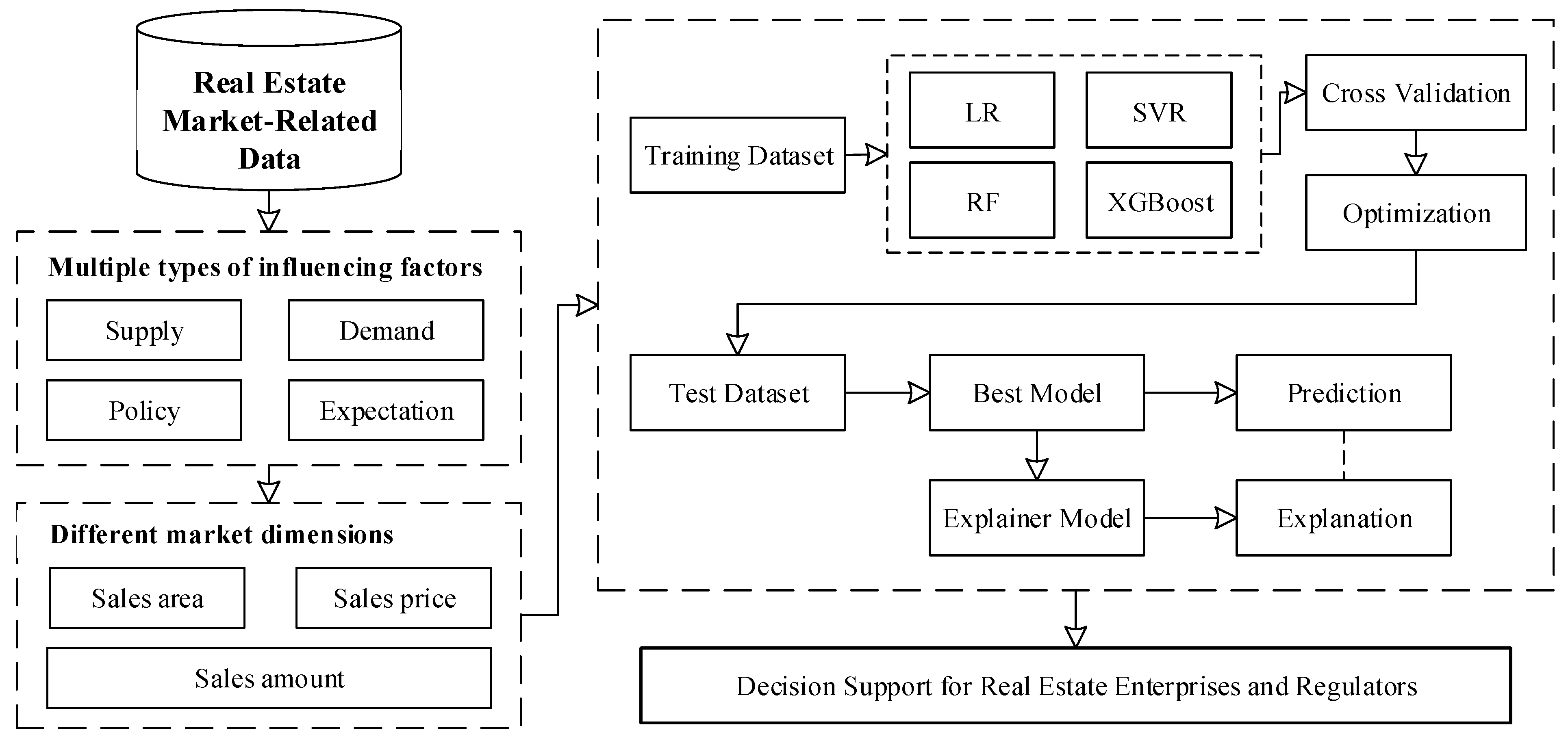
3. Methods
3.1. Machine Learning Models
- (1)
- Support Vector Regression (SVR)
- (2)
- Random Forest (RF)
- (3)
- Extreme Gradient Boosting (XGBoost)
- (4)
- Explainable Artificial Intelligence (XAI)
3.2. Market Forecasting Indicator System
- (1)
- Supply Factors
- (2)
- Demand Factors
- (3)
- Policy Factors
- (4)
- Expectation Factors
3.3. Model Evaluation Metrics
4. Explainable Machine Learning Model Construction
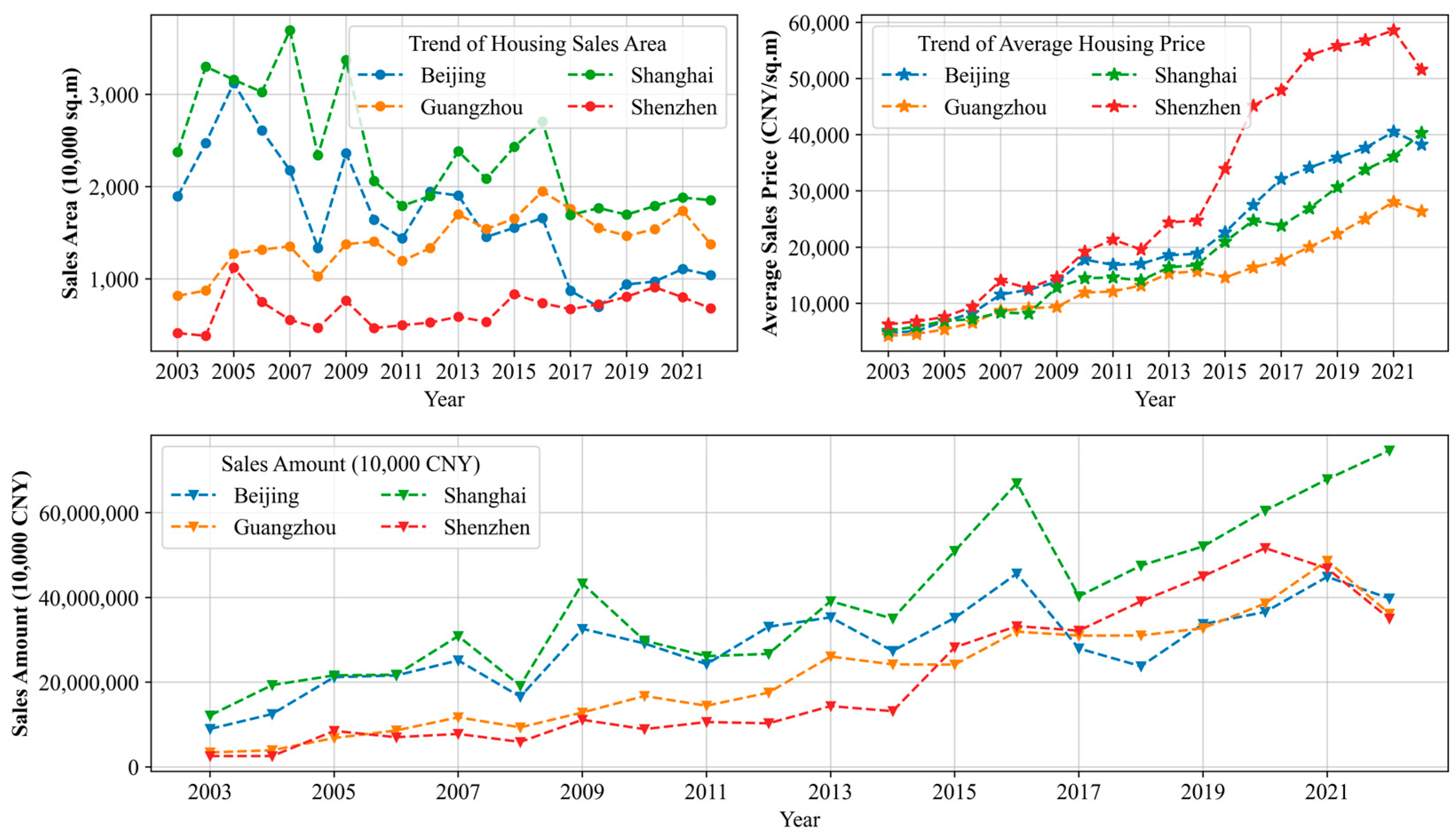
4.1. Data Collection and Preprocessing
4.2. Model Training and Evaluation
- (1)
- Data Preprocessing
- (2)
- Model Construction
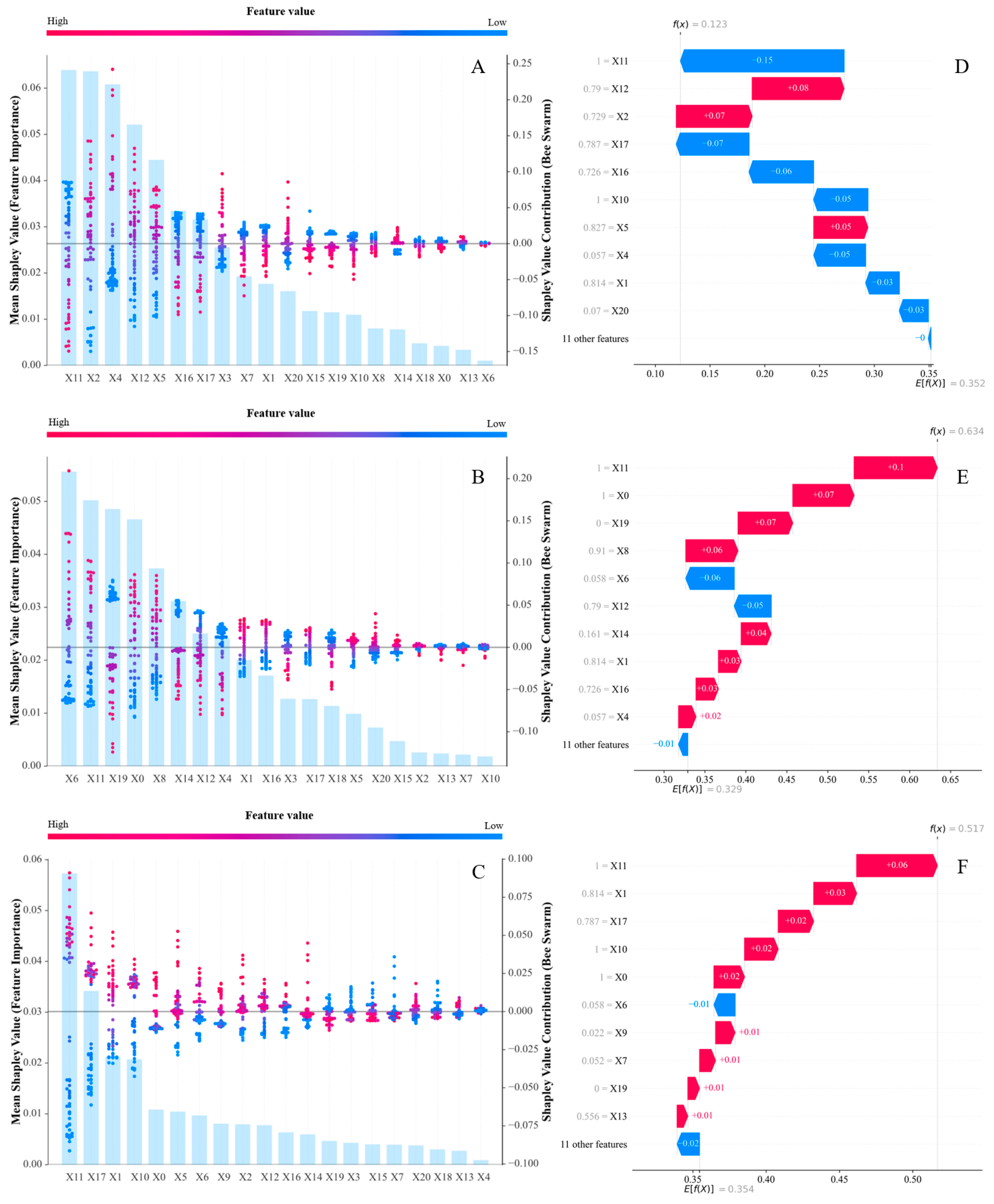
4.3. Analysis of Key Influencing Factors
- (1)
- Key Factors Influencing Commercial Housing Sales Area
- (2)
- Key Factors Influencing Commercial Housing Average Sales Price
- (3)
- Key Factors Influencing Commercial Housing Sales Amount
- (4)
- Case Study on Influencing Factors
5. Conclusions and Discussion
5.1. Research Findings
5.2. Theoretical Contributions
5.3. Implications
5.4. Limitations and Future Research Directions
Author Contributions
Funding
Data Availability Statement
Acknowledgments
Conflicts of Interest
References
- Chen, X.; Chen, Y. Evaluation and Improvement Strategies of the Long-Term Mechanism for Real Estate: A Perspective of the “Three-in-One” Macro Policy Approach. Stud. Explor. 2022, 8, 99–112. [Google Scholar]
- Chen, X.; Cheng, S.; Chen, K.; Xiao, Z.Y. A Study on the Influencing Factors of Housing Prices in First-Tier Cities Based on Machine Learning Methods. Nankai J. Philos. Soc. Sci. 2023, 6, 146–163. [Google Scholar]
- Gong, J.; Zheng, T. Investor Attention and Intercity Housing Price Spillover Effects: A Study Based on Baidu Search Index Between Pair Cities. J. Financ. Econ. 2023, 6, 55–70. [Google Scholar]
- Liu, S.; Chen, M. Study on the Transmission Effect of Chinese Urban Housing Price Fluctuation Diffusion Level. Reg. Res. Dev. 2021, 40, 45–50. [Google Scholar]
- Cui, Z.; Zhou, M.; Kong, L. Study on the Heterogeneity of Influencing Factors of Urban Housing Prices in China. Tax Econ. 2022, 6, 65–74. [Google Scholar]
- Paulus, N.M.; Lautenschlaeger, L.; Schaefers, W. Social Media and Real Estate: Do Twitter Users Predict REIT Performance? J. Real Estate Res. 2024, 1, 1–34. [Google Scholar] [CrossRef]
- Alhefnawei, A.M.M.; Al, E. Population Modeling and Housing Demand Prediction for the Saudi 2030 Vision: A Case Study of Riyadh City. Int. J. Hous. Mark. Anal. 2024, 17, 1558–1572. [Google Scholar] [CrossRef]
- Wang, X.-R.; Hui, E.C.-M.; Sun, J.-X. Population Migration, Urbanization and Housing Prices: Evidence from the Cities in China. Habitat Int. 2017, 66, 49–56. [Google Scholar] [CrossRef]
- Du, H.; Xu, M.; Wang, Y.; Chen, L. Housing wellbeing and settlement intentions of skilled migrants in China: The effects of subjective housing feelings and objective housing outcomes. Appl. Spat. Anal. Policy 2024, 17, 983–1015. [Google Scholar] [CrossRef]
- Long, J.; Cui, C.; Kohl, S.; Yang, Y. The ladder of prosperity: An analysis of housing wealth accumulation across income groups in urban China. China Econ. Rev. 2025, 92, 102428. [Google Scholar] [CrossRef]
- Lin, X.; Lü, P. Research on the Spatial Correlation and Influencing Factors of Housing Prices in the Beijing-Tianjin-Hebei Urban Agglomeration Based on the Spatial Durbin Model. Econ. Prob. Explor. 2021, 1, 79–90. [Google Scholar]
- Shen, S.; Zhao, Y.; Pang, J. Local Housing Market Sentiments and Returns: Evidence from China. J. Real Estate Financ. Econ. 2024, 68, 488–522. [Google Scholar] [CrossRef]
- Cheng, Y.; Li, H.; Dai, Y.; Xu, Y.F. Stock Market Volatility and Urban Housing Prices: An Empirical Analysis Based on Monthly Panel Data from 2011 to 2017. Econ. Sci. 2025, 1, 27–47. [Google Scholar]
- Lu, J.; Liu, F.; Hua, Y. Monetary Policy, Stock Prices, and Housing Price Volatility. Stat. Inf. Forum 2023, 38, 81–94. [Google Scholar]
- Wu, W.; Zhou, A. Causes of Housing Price Fluctuations: Demand Rigidity or Land Finance? Shandong Soc. Sci. 2021, 3, 126–132. [Google Scholar]
- Li, Z.; Zhang, H. Cost Push, Demand Pull: What Has Driven the Increase in Housing Prices in China? China Manag. Sci. 2015, 23, 143–150. [Google Scholar]
- Wu, J.; Li, H.; Hu, B. The Impact of Land Cost on the Price of Newly Built Commercial Housing. Price Theor. Pract. 2015, 9, 52–54. [Google Scholar]
- Melecky, A.; Paksi, D. Drivers of European Housing Prices in the New Millennium: Demand, Financial, and Supply Determinants. Empirica 2024, 51, 731–753. [Google Scholar] [CrossRef]
- Chen, S.; Zhu, W. The Impact of Sheltered Housing Monetization on the Real Estate Market. Jianghan Forum 2024, 6, 33–42. [Google Scholar]
- Cui, M.; Liu, X.; Li, X.; Dong, J.C. Data-Driven Integrated Prediction of the Real Estate Market. Manag. Rev. 2020, 32, 89–101. [Google Scholar]
- Yakub, A.A.; Al, E. An Analysis of the Determinants of Office Real Estate Price Modeling in Nigeria: Using a Delphi Approach. Prop. Manag. 2022, 40, 758–779. [Google Scholar]
- Wang, Q.; Gu, L.; Guo, H. Analysis and Forecast of Housing Price Cycles in First-Tier Cities in China. Price Theor. Pract. 2014, 5, 55–57. [Google Scholar]
- Liu, D.; Wang, W.; Xie, H.; Wang, S.Y.; Lu, F.B. Analysis and Forecast of Influencing Factors of Real Estate Prices in China. Manag. Rev. 2010, 22, 3–10. [Google Scholar]
- Rapach, D.E.; Strauss, J.K. Differences in Housing Price Forecast Ability Across U.S. States. Int. J. Forecast. 2009, 25, 351–372. [Google Scholar] [CrossRef]
- Yang, G.; Luo, Y.; Gao, J. Study on Housing Price Forecasting Models in China. Stat. Decis. 2014, 12, 17–20. [Google Scholar]
- Kouwenberg, R.; Zwinkels, R. Forecasting the U.S. Housing Market. Int. J. Forecast. 2014, 30, 415–425. [Google Scholar] [CrossRef]
- Liu, C.; Yao, J. Real Estate Price Forecasting Model Based on Multiple Factors. Stat. Decis. 2017, 17, 33–38. [Google Scholar]
- Shi, J.; Xiao, Y. An Evaluation Model for Second-Hand Housing Prices Based on Urban Big Data. China Manag. Sci. 2025, 1, 1–17. [Google Scholar]
- Chen, X.; Chen, K.; Wang, Z.; Xiao, Z.Y. Factors Affecting Housing Price Differentiation Among Cities. Econ. Theor. Econ. Manag. 2024, 44, 49–64. [Google Scholar]
- Habbab, F.Z.; Kampouridis, M. An In-Depth Investigation of Five Machine Learning Algorithms for Optimizing Mixed-Asset Portfolios Including REITs. Expert Syst. Appl. 2024, 235, 121102. [Google Scholar] [CrossRef]
- Tang, X.; Zhang, R.; Liu, L. Research on the Forecasting of Beijing’s Second-Hand Housing Prices Based on Bat Algorithm and SVR Model. Stat. Res. 2018, 35, 71–81. [Google Scholar]
- Zhang, W.; Ma, L. Research on Urban Second-Hand Housing Price Evaluation Method: An Analysis of Beijing’s Second-Hand Housing Prices Based on Lasso-GM-RF Combined Model. Price Theor. Pract. 2020, 9, 172–175+180. [Google Scholar]
- Shokoohyar, S.; Sobhani, A.; Sobhani, A. Determinants of Rental Strategy: Short-Term vs Long-Term Rental Strategy. Int. J. Contemp. Hosp. Manag. 2020, 32, 3873–3894. [Google Scholar] [CrossRef]
- Guliker, E.; Folmer, E.; van Sinderen, M. Spatial Determinants of Real Estate Appraisals in the Netherlands: A Machine Learning Approach. ISPRS Int. J. Geo-Inf. 2022, 11, 125. [Google Scholar] [CrossRef]
- Lundberg, S.M.; Lee, S.I. A Unified Approach to Interpreting Model Predictions. Adv. Neural Inf. Process. Syst. 2017, 30. [Google Scholar]
- Li, L.; Fu, B. Study on Real Estate Bubble Measurement in China Based on Beijing Data. Commer. Res. 2011, 3, 61–67. [Google Scholar]
- Tang, L.Z.; Zhu, J.F.; Luo, J. A New Measurement of the Influencing Factors of Real Estate Prices from the Perspective of Macroeconomic Regulation. Econ. Theor. Econ. Manag. 2014, 1, 102–107. [Google Scholar]
- Li, J.N.; You, W.X.; Sun, P.Y. Does In-Migration Promote Housing Price Increases in Cities? An Empirical Study Based on Chinese Urban Data. Nankai Econ. Stud. 2017, 1, 58–76. [Google Scholar]
- Li, J.L. Study on the Influencing Factors of Housing Price Fluctuations: An Empirical Analysis Based on 2005–2015 Data. Econ. Theor. Econ. Manag. 2017, 9, 30–37. [Google Scholar]
- Gao, Y.; Li, X.T.; Dong, J.C. Why Do Housing Prices Differ in Cities? The Impact of Public Services on Housing Prices. Syst. Eng. Theor. Pract. 2019, 39, 2255–2262. [Google Scholar]
- Tang, Y.G.; Chen, Q.; Man, L.P. Capitalization, Fiscal Incentives, and Local Public Service Provision: An Empirical Analysis Based on 35 Medium and Large Cities in China. Econ. Q. J. 2016, 15, 217–240. [Google Scholar]
- Liu, C.; Yang, J.D. Strategic Land Supply and Housing Price Differentiation. Financ. Res. 2019, 45, 68–82. [Google Scholar]
- Li, F.; Shi, Y.N.; Xu, Z.H.; Zhang, H.Y. Credit and Housing Prices: The Impact of First-Time Home Loan Rates on Housing Prices in China. J. Southwest Univ. (Soc. Sci.) 2022, 43, 132–142. [Google Scholar]
- Shi, Y.N.; Wang, J.; Ye, J.P. The Pathway of Housing Price Increase: A Re-Verification of Fiscal Policy, Population, and Expectations. J. Zhejiang Gongshang Univ. 2021, 2, 94–106. [Google Scholar]
- Gao, B.; Wang, H.L.; Li, W.J. Expectations, Speculation, and Housing Price Bubbles in Chinese Cities. Financ. Res. 2014, 2, 44–58. [Google Scholar]
- Dong, J.C.; He, J.; Li, X.T.; Dong, Z. The Mechanism of Public Housing Price Expectation Formation: An Empirical Study Based on Social Learning Perspective. Manag. Rev. 2020, 32, 34–46. [Google Scholar]
- Hu, L.; He, S.; Han, Z.; Xiao, H.; Su, S.; Weng, M.; Cai, Z. Monitoring Housing Rental Prices Based on Social Media: An Integrated Approach of Machine-Learning Algorithms and Hedonic Modeling to Inform Equitable Housing Policies. Land Use Policy 2019, 82, 657–673. [Google Scholar] [CrossRef]
- Rico-Juan, J.R.; de La Paz, P.T. Machine Learning with Explainability or Spatial Hedonics Tools? An Analysis of the Asking Prices in the Housing Market in Alicante, Spain. Expert Syst. Appl. 2021, 171, 114590. [Google Scholar] [CrossRef]
- Baur, K.; Rosenfelder, M.; Lutz, B. Automated Real Estate Valuation with Machine Learning Models Using Property Descriptions. Expert Syst. Appl. 2023, 213, 119147. [Google Scholar] [CrossRef]
- Yan, X.X.; Xia, E.J. Forecasting the Sales Area of Ordinary Residential Commercial Houses in Beijing. J. Beijing Inst. Technol. (Soc. Sci.) 2002, S1, 88–90. [Google Scholar]
- Wang, X.Z.; Shao, J.; Hong, J.K.; Chen, M.K. A Short-Term Housing Price Forecasting Method Integrating Multi-Source Heterogeneous Information and Data Features. Syst. Eng. Theor. Pract. 2025, 1, 1–20. [Google Scholar]
- Friedman, M. The use of ranks to avoid the assumption of normality implicit in the analysis of variance. J. Am. Stat. Assoc. 1937, 32, 675–701. [Google Scholar] [CrossRef]
- Gold, C.; Holub, A.; Sollich, P. Bayesian Approach to Feature Selection and Parameter Tuning for Support Vector Machine Classifiers. Neural Netw. 2005, 18, 693–701. [Google Scholar] [CrossRef] [PubMed]
- Zhou, X.J.; Gu, X. Robust Parameter Design Based on Bayesian Support Vector Regression Machine. Stat. Decis. 2023, 39, 23–28. [Google Scholar]

| Factor Category | Indicator Name | Variable | Data Source |
|---|---|---|---|
| Supply Factors | Real estate development investment amount | National Bureau of Statistics | |
| Floor area under construction by real estate developers | |||
| Completed floor area by real estate developers | |||
| Land area purchased by real estate developers | |||
| Demand Factors | Permanent population | China Urban Statistical Yearbook | |
| Population density | |||
| Natural population growth rate | |||
| Per capita GDP | |||
| Per capita disposable income | |||
| Household deposit balance | National Bureau of Statistics | ||
| Educational expenditure | China Urban Statistical Yearbook | ||
| Number of hospital beds | |||
| Urban road area | |||
| Park green space area | |||
| Urban green coverage ratio | |||
| Policy Factors | General public budget revenue | ||
| General public budget expenditure | |||
| General public fiscal deficit ratio | Estimated data | ||
| National benchmark interest rate for loans over 5 years | People’s Bank of China | ||
| Expectation Factors | House price growth rate (lagging one period) | Estimated data |
| Real Estate Market Indicator | Unit | Min. | Mean | Max. |
|---|---|---|---|---|
| Commercial Housing Sales Amount | CNY 10,000 | 2,575,595.20 | 27,565,412.08 | 74,674,769.76 |
| Commercial Housing Sales Area | 10,000 sq. m | 381.69 | 1524.10 | 3694.96 |
| Commercial Housing Average Sales Price | CNY/sq. m | 4211.00 | 20,742.84 | 58,593.00 |
| Task | Model | Evaluation Metrics | |||||
|---|---|---|---|---|---|---|---|
| Commercial Housing Sales Area | LR | 3.5969 | 1543.16% | 0.5674 | 243.42% | −254.7684 | 0.8614 |
| SVR | 0.1305 | 55.97% | 0.1003 | 43.04% | 0.6856 | 0.8498 | |
| RF | 0.1418 | 60.83% | 0.1005 | 43.12% | 0.6287 | 0.8431 | |
| XGBoost | 0.1523 | 65.36% | 0.1120 | 48.06% | 0.5706 | 0.8237 | |
| Commercial Housing Average Sales Price | LR | 1.4724 | 546.64% | 0.2613 | 97.01% | −34.5733 | 0.8115 |
| SVR | 0.0905 | 33.60% | 0.0734 | 27.27% | 0.8868 | 0.8603 | |
| RF | 0.0946 | 35.11% | 0.0677 | 25.12% | 0.8756 | 0.8214 | |
| XGBoost | 0.1141 | 42.35% | 0.0720 | 26.73% | 0.8170 | 0.8047 | |
| Commercial Housing Sales Amount | LR | 2.5017 | 1128.55% | 0.4080 | 184.07% | −139.0169 | 0.8424 |
| SVR | 0.1063 | 47.97% | 0.0817 | 36.86% | 0.7691 | 0.8563 | |
| RF | 0.1047 | 47.24% | 0.0810 | 36.54% | 0.7762 | 0.8881 | |
| XGBoost | 0.1117 | 50.39% | 0.0865 | 39.03% | 0.7443 | 0.8712 | |
| Task | Model | Average Rank of Evaluation Metrics | |||||
|---|---|---|---|---|---|---|---|
| Commercial Housing Sales Area | LR | 4.00 | 4.00 | 4.00 | 4.00 | 4.00 | 1.55 |
| SVR | 1.05 | 1.05 | 1.56 | 1.56 | 1.05 | 2.24 | |
| RF | 2.09 | 2.09 | 1.56 | 1.56 | 2.09 | 2.63 | |
| XGBoost | 2.86 | 2.86 | 2.88 | 2.88 | 2.86 | 3.58 | |
| 279.012 | 279.012 | 249.696 | 249.696 | 279.012 | 90.589 | ||
| p-Value | 0.000 | 0.000 | 0.000 | 0.000 | 0.000 | 0.000 | |
| Commercial Housing Average Sales Price | LR | 4.00 | 4.00 | 4.00 | 4.00 | 4.00 | 2.69 |
| SVR | 1.46 | 1.46 | 2.44 | 2.44 | 1.46 | 1.18 | |
| RF | 1.70 | 1.70 | 1.39 | 1.39 | 1.70 | 2.67 | |
| XGBoost | 2.84 | 2.84 | 2.17 | 2.17 | 2.84 | 3.46 | |
| 245.232 | 245.232 | 215.676 | 215.676 | 245.232 | 142.750 | ||
| p-Value | 0.000 | 0.000 | 0.000 | 0.000 | 0.000 | 0.000 | |
| Commercial Housing Sales Amount | LR | 4.00 | 4.00 | 4.00 | 4.00 | 4.00 | 3.12 |
| SVR | 1.95 | 1.95 | 1.81 | 1.81 | 1.95 | 2.86 | |
| RF | 1.53 | 1.53 | 1.59 | 1.59 | 1.53 | 1.46 | |
| XGBoost | 2.52 | 2.52 | 2.60 | 2.60 | 2.52 | 2.56 | |
| 209.628 | 209.628 | 213.852 | 213.852 | 209.628 | 136.782 | ||
| p-Value | 0.000 | 0.000 | 0.000 | 0.000 | 0.000 | 0.000 | |
| Task | Metrics | Hyperparameters | ||||||||
|---|---|---|---|---|---|---|---|---|---|---|
| C | Gamma | Kernel | ||||||||
| Commercial Housing Sales Area | 0.1084 | 46.60% | 0.0863 | 37.10% | 0.7827 | 0.8421 | 1.0 | “scale” | “rbf” | |
| 0.1002 | 43.05% | 0.0789 | 33.91% | 0.8146 | 0.8947 | 14.8915 | 0.0174 | “rbf” | ||
| Commercial Housing Average Sales Price | 0.0898 | 46.23% | 0.0803 | 41.43% | 0.7855 | 1.0000 | 1.0 | “scale” | “rbf” | |
| 0.0770 | 39.73% | 0.0639 | 32.98% | 0.8422 | 1.0000 | 73.9421 | 0.1124 | “rbf” | ||
| Task | MD | MSL | MSS | NE | ||||||
| Commercial Housing Sales Amount | 0.0806 | 35.43% | 0.0551 | 24.23% | 0.8745 | 0.8947 | None | 1 | 2 | 100 |
| 0.0796 | 35.02% | 0.0529 | 23.26% | 0.8774 | 0.8947 | 4 | 1 | 2 | 150 | |
Disclaimer/Publisher’s Note: The statements, opinions and data contained in all publications are solely those of the individual author(s) and contributor(s) and not of MDPI and/or the editor(s). MDPI and/or the editor(s) disclaim responsibility for any injury to people or property resulting from any ideas, methods, instructions or products referred to in the content. |
© 2025 by the authors. Licensee MDPI, Basel, Switzerland. This article is an open access article distributed under the terms and conditions of the Creative Commons Attribution (CC BY) license (https://creativecommons.org/licenses/by/4.0/).
Share and Cite
Song, D.; Hu, G.; Li, H.; Zhao, H.; Wang, Z.; Liu, Y. Real Estate Market Forecasting for Enterprises in First-Tier Cities: Based on Explainable Machine Learning Models. Systems 2025, 13, 513. https://doi.org/10.3390/systems13070513
Song D, Hu G, Li H, Zhao H, Wang Z, Liu Y. Real Estate Market Forecasting for Enterprises in First-Tier Cities: Based on Explainable Machine Learning Models. Systems. 2025; 13(7):513. https://doi.org/10.3390/systems13070513
Chicago/Turabian StyleSong, Dechun, Guohui Hu, Hanxi Li, Hong Zhao, Zongshui Wang, and Yang Liu. 2025. "Real Estate Market Forecasting for Enterprises in First-Tier Cities: Based on Explainable Machine Learning Models" Systems 13, no. 7: 513. https://doi.org/10.3390/systems13070513
APA StyleSong, D., Hu, G., Li, H., Zhao, H., Wang, Z., & Liu, Y. (2025). Real Estate Market Forecasting for Enterprises in First-Tier Cities: Based on Explainable Machine Learning Models. Systems, 13(7), 513. https://doi.org/10.3390/systems13070513