A Life-Cycle Carbon Reduction Optimization Framework for Production Activity Systems: A Case Study on a University Campus

Abstract

Decarbonizing production activities is a critical task in the transition towards carbon neutrality. Traditional carbon footprint accounting tools, such as life-cycle assessment (LCA) and the Greenhouse Gas Protocol, primarily quantify direct and indirect emissions but offer limited guidance on actionable reduction strategies. To address this gap, this study proposes a comprehensive life-cycle carbon footprint optimization framework that integrates LCA with a mixed-integer linear programming (MILP) model. The framework, while applicable to various production contexts, is validated using a university campus as a case study. In 2023, the evaluated university’s net carbon emissions totaled approximately 24,175.07 t CO₂-eq. Based on gross emissions (28,306.43 t CO₂-eq) before offsetting, electricity accounted for 66.09%, buildings for 15.55%, fossil fuels for 8.67%, and waste treatment for 8.46%. Seasonal analysis revealed that June and December exhibited the highest energy consumption, with emissions exceeding the monthly average by 19.4% and 48.6%, respectively, due to energy-intensive air conditioning demand. Teaching activities emerged as a primary contributor, with baseline emissions estimated at 5485.24 t CO₂-eq. Optimization strategies targeting course scheduling yielded substantial reductions: photovoltaic-based scheduling reduced electricity emissions by 7.00%, seasonal load shifting achieved a 26.92% reduction, and combining both strategies resulted in the highest reduction, at 45.95%. These results demonstrate that aligning academic schedules with photovoltaic generation and seasonal energy demand can significantly enhance emission reduction outcomes. The proposed framework provides a scalable and transferable approach for integrating time-based and capacity-based carbon optimization strategies across broader operational systems beyond the education sector.

1. Introduction

Global climate change has become one of the most pressing environmental issues of the 21st century. The Paris Agreement aims to limit the global temperature rise to well below 2 °C above pre-industrial levels, preferably within 1.5 °C [1], and achieve global climate neutrality by the middle of this century. Some major economies such as China, EU and Japan have set ambitious carbon neutrality targets, necessitating substantial emissions reductions across all sectors [2]. Current climate action primarily focuses on transitioning to renewable energy sources as a replacement for fossil fuel combustion [3]. However, these efforts alone remain insufficient due to fundamental challenges, including the inherent intermittency of renewables and the prohibitively high costs of large-scale energy storage systems [4]. Therefore, a more systematic and multi-faceted approach from consumption sides is essential to minimizing the carbon footprint of human activities [5].

Carbon accounting and emission reduction are inherently multi-scale challenges, spanning global, national, regional, and organizational levels [6]. Among these, regional-scale carbon management plays a practical role in bridging macro-level climate policies with localized decarbonization actions [7], ensuring more effective and context-specific mitigation strategies. In particular, regional carbon footprints often encompass multiple emission sources, including industrial [8,9], commercial [10], transportation [10,11], and residential [12,13], adding layers of complexity to accurate measurement and targeted reduction efforts. By employing precise carbon footprint evaluation and data-driven optimization, regional carbon management can generate actionable insights for integrating renewable energy and optimizing resource utilization. Moreover, it also helps guide sector-specific decarbonization pathways and accelerates the transition toward a low-carbon society.

Regional carbon management employs several accounting methods, including Input–Output Analysis (IOA) [14,15], the Green Gas Protocol (GHG Protocol) [16], and life-cycle assessment (LCA) [17,18,19]. IOA is primarily designed for global and national-scale studies, and its coarse granularity makes it ill-suited for formulating precise local decarbonization measures [15]. The GHG Protocol, widely adopted as a framework, categorizes emissions into direct and indirect groups. It effectively quantifies direct emissions and certain indirect energy-related emissions [14], such as those from electricity use, yet it struggles to capture the diffuse and heterogeneous emissions encompassed in Scope 3, like those arising from services or investments. In contrast, LCA offers a more detailed evaluation by focusing on the material and energy inputs and outputs of processes, making it particularly promising for carbon footprint optimization. However, the effectiveness of LCA in guiding emission reduction strategies is limited because it often lacks a comprehensive understanding of the underlying process mechanisms that drive these emissions. Therefore, it is essential to integrate LCA-based carbon accounting with an evaluation of the impacts of various design and operational factors to develop actionable optimization strategies.

In order to bridge the gap between carbon accounting and decarbonization actions, we use university campuses as a case study to develop a novel regional carbon optimization approach. Recognizing that university operations exhibit similarities to urban structures [20], we regard these campuses as “miniature cities”. Moreover, as important carriers of green, low-carbon education, university campuses play a pivotal role in shaping public awareness through their carbon measurement and emission reduction initiatives. For instance, the Ministry of Education of China has introduced the “Implementation Plan for the Construction of a Green Low-carbon National Education System”, which integrates green low-carbon development principles into campus construction. Urban carbon management traditionally employs zonal modeling based on functional areas, such as residential, commercial, and industrial zones, to develop targeted reduction strategies. Similarly, university campuses, which can be viewed as miniature cities, consist of diverse functional areas including academic, residential, laboratory, administrative, and transportation zones, each exhibiting distinct carbon emission patterns. For complex regional carbon footprint assessments and the planning of emission reduction pathways, a standardized framework that integrates detailed carbon accounting with an analysis of variable operational factors is necessary. By identifying emission hotspots and considering the dynamic nature of production and activity patterns, such a framework can inform the development of actionable and optimized decarbonization strategies tailored to the region’s complexities.

Existing studies on university carbon footprints have highlighted three key research gaps. First, while some studies have addressed economic impacts, energy consumption [21], and per capita emissions [22], relatively few have conducted comprehensive campus-wide carbon footprint assessments using standardized metrics and functional segmentation [22]. Helmers et al. (2021) [21] compared global university emissions using harmonized indicators and found that differences in national energy policies significantly affect per capita carbon footprints. However, most current methodologies struggle to categorize and quantify emissions across diverse operational functions. For example, Clabeaux et al. (2020) [22] adopted a life-cycle approach but focused more on building-level aggregation than activity-based breakdowns. Recent research has also explored energy optimization strategies at the campus level. Wang et al. (2023) [23] examined photovoltaic (PV) integration and Heating, Ventilation, and Air Conditioning (HVAC) control for Chinese universities, identifying practical gaps in emission reductions despite policy commitments. Meanwhile, Helmers et al. (2022) [24] quantified embodied emissions from infrastructure and procurement, further expanding the boundary of university carbon inventories. Ridhosari and Rahman (2020) [25] and Charles et al. (2022) [26] emphasized emissions from electricity and transport but lacked detailed modeling of operational scheduling impacts. Second, although prior work has quantified campus-wide electricity use [20,25,27], few studies have analyzed how teaching-related variables, such as course schedules, classroom occupancy, class-hour clustering, and seasonal load shifts, affect carbon emissions. Guerrieri et al. (2019) [20] focused on long-term carbon transition paths but did not incorporate temporal scheduling dynamics. Ridhosari and Rahman (2020) [25] conducted scope-based footprint accounting without disaggregating teaching processes. Ozawa-Meida et al. (2013) [27] adopted a consumption-based approach yet lacked the modeling of intra-semester variations. Helmers et al. (2022) [24] expanded the boundary of campus footprints to embodied emissions but treated educational activities as a static demand. Charles et al. (2022) [26] and Liu et al. (2024) [28] emphasized holistic planning and ecological indicators, respectively, without linking teaching operations to energy patterns. In contrast, this study explicitly models teaching activities as spatiotemporal operational units, linking them to carbon emission sources through a multi-dimensional optimization framework. By incorporating dynamic scheduling parameters and coupling them with classroom energy profiles and PV generation data, the proposed method enables strategy-based emission reduction simulations under realistic teaching constraints. Third, mathematical optimization has not yet been widely applied to university decarbonization. While automated timetabling has been studied extensively for logistical efficiency [29], and MILP has been used to build energy systems [30], few studies have leveraged such tools to design low-carbon scheduling frameworks in academic contexts. Burke et al. (2010) [29] developed hybrid metaheuristics for university exam timetabling, aiming to satisfy complex constraints and improve allocation robustness. However, carbon optimization objectives remain largely absent in existing scheduling frameworks.

To support the development of a scalable carbon footprint optimization framework for university campuses, this study integrates LCA-based carbon accounting approaches—with mathematical optimization techniques. It evaluates key emission sources, including building construction, operational energy consumption, and waste treatment. Teaching activities are identified as a primary emission hotspot, and a mixed-integer linear programming (MILP) model is developed to optimize the allocation of teaching resources and schedules. Beyond quantifying emissions under realistic constraints, this study also examines the effectiveness of multiple decarbonization strategies, such as PV-aligned scheduling and spatial utilization optimization, providing practical insights for low-carbon campus operations. The methodology, validated through a single-campus case, is adaptable to universities of varying sizes, geographic contexts, and energy structures. It also offers a replicable strategy that can be extended into region-wide, life-cycle-oriented carbon management models, ultimately contributing to urban sustainability by minimizing emissions without compromising core operational functions.

The structure of this paper is organized as follows: Section 2 introduces the carbon footprint accounting methodology and datasets. Section 3 presents the modeling framework and optimization strategies. Section 4 discusses the results and implications. Section 5 concludes with key findings and outlines future research directions.

2. Method

2.1. Research Framework for Regional Carbon Optimization Model

In this study, we conceptualize a university’s campus and teaching operations as a structured production activity system, where individual courses are treated as discrete tasks requiring coordinated spatial (classroom), temporal (timeslot), and energy (electricity, HVAC) resources. Although the model was developed based on educational activities, this framework can be extended to industrial production systems, where operations such as manufacturing or batch processing must also be scheduled using constrained resources. This abstraction supports the use of optimization tools such as MILP and facilitates the potential extension of the framework to industrial, commercial, and urban-scale applications.

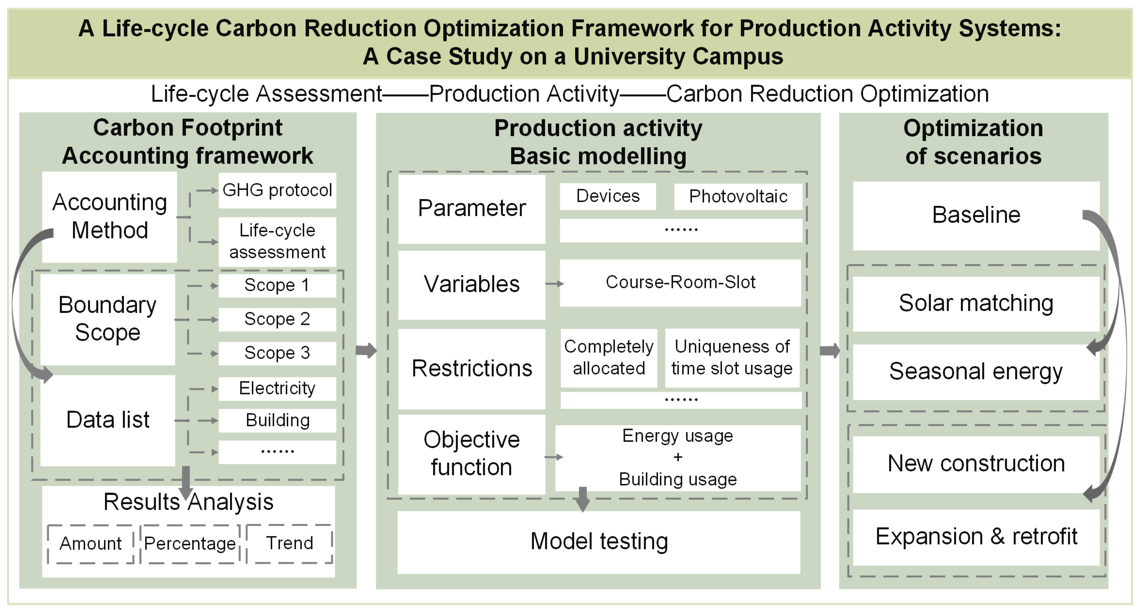
To facilitate regional and organizational carbon reduction [31], this study proposes an extendable framework that integrates accounting, modeling, and optimization for carbon footprint. This framework combines life-cycle inventory analysis, dynamic activity modeling, and the development of optimized reduction strategies. To demonstrate its applicability, we apply the framework to a case study of university campuses. This approach systematically quantifies the campus carbon footprint and optimizes teaching activities to meet carbon reduction targets. The framework’s structure is illustrated in Figure 1.

Based on the GHG Protocol, the carbon footprint of the evaluated university is calculated across three scopes. Scope 1 includes direct emissions from fossil fuel combustion for domestic hot water, cafeteria operations, and school bus usage, as well as negative emissions from carbon sinks. Scope 2 accounts for indirect emissions from purchased electricity consumption, incorporating PV generation. Scope 3 covers the carbon footprint of building construction and waste management. In this study, the carbon footprint accounting scope of Shanghai University of Engineering Science is calculated as an example, demonstrating that this method can be widely applied to similar campuses and regions. The case study focuses on the Songjiang Campus of Shanghai University of Engineering Science, which covers approximately 783,000 m² with a total floor area of 538,000 m². The campus hosts around 16,000 students and 1500 staff across diverse functional buildings, including 12 teaching buildings and 8 laboratories. Teaching and lab areas account for 62% of the building area and constitute the major sources of energy consumption and carbon emissions.

Given that teaching activities represent the core production process on university campuses, they serve as a critical focus for our model. To clarify the research scope, this model focuses exclusively on regular teaching schedules within standard academic semesters. Temporary adjustments such as holidays, emergency responses, or ad hoc meetings are excluded from the modeling boundary, as they represent exceptional operational variations rather than typical production activities. Teaching activities drive daily operations and account for significant resource consumption and energy use. Building on the carbon footprint assessment, we conceptualize each course session as a production task that requires specific resources, such as classrooms, time slots, and energy, over designated periods. In the modeling stage, two key aspects are addressed. First, the model optimizes scheduling [32] by matching courses with appropriate classrooms and time slots, taking into account constraints like classroom capacity, institutional scheduling policies, and availability. Second, it integrates calculations of energy consumption and building carbon footprints, incorporating both operational energy use [33] and the embodied carbon associated with the physical infrastructure. This dual approach enables comprehensive analysis that supports both immediate operational improvements and long-term campus planning, ultimately laying the groundwork for evidence-based decisions aimed at reducing overall carbon emissions while upholding educational standards.

Based on the established model, the optimization phase aims to reduce the university’s carbon footprint by exploring multiple operational strategies. First, a baseline strategy reflecting the current teaching schedule is defined to quantify existing emissions and operational constraints. Within this baseline, a fundamental optimization strategy involves adjusting the teaching schedule to avoid clustering classes during high-energy-consumption periods, thereby reducing peak carbon intensity. In another strategy, rooftop PV systems are integrated with the teaching schedule to offset carbon emissions by supplying renewable energy during periods of high demand. Additionally, when considering variable classroom resources under cases such as, new construction, renovations, and campus expansion, the trade-offs are evaluated between increased teaching capacity and the associated building emissions. Together, these strategies enable a comprehensive assessment of emission reduction measures and pave the way for a dynamic carbon management plan that aligns with both current operations and future campus development.

2.2. Carbon Footprint Modeling of a Campus

According to the GHG Protocol and standards ISO 14040 [34], ISO 14067 [35], and ISO 14064-1/2/3 [36,37,38], we developed a model for accounting the carbon footprint of a campus. In our approach, Scope 1 emissions are calculated using the emission factor method, while Scope 2 and 3 emissions are determined through LCA.

Table 1. Data sources of inventory analysis for the carbon footprint accounting of universities.

Categories	Foreground Data Sources	Background Data Sources
Fuel (Scope 1)	Canteen gas, boiler heating, official vehicle fuel	Ecoinvent
Carbon sink (Scope 1)	Campus green space	Government standards
Purchased electricity from grid [39] (Scope 2)	Purchased power consumption (lighting, HVAC, labs, infrastructure power)	Ecoinvent
Distributive PV electricity (Scope 2)	Rooftop PV installation and power generation	Ecoinvent
Building (Scope 3)	Building materials used in various types of buildings	Ecoinvent, Literature, CLCD
Waste treatment [40] (Scope 3)	Dry, organic, water [41] waste	Ecoinvent, CLCD
Offset	Recyclable waste, PV grid-connected electricity	CLCD

summarizes the detailed contributions of these emission categories to the overall campus carbon footprint.

Carbon footprint calculation is based on foreground data and background data. Foreground data includes campus energy billing records (Table S1 in Supporting Information (SI)), GIS map data (covering building footprint area and green space area), statistical data (such as vegetation types, building floor levels) (Tables S2 and S3 in Supporting Information), and literature sources (Table S4 in Supporting Information).

Background data of building materials, energy, and waste treatments primarily comes from the Ecoinvent [42] database, the Chinese Life Cycle Database (CLCD) (Table S5 in Supporting Information). The carbon emission factors of fuel combustion, carbon sequestration calculation are based on government standards [43] (Table S6 in Supporting Information). The total carbon footprint can be calculated using Equation (1).

$$C{F}_{total}=C{F}_{Scope1}+C{F}_{Scope2}+C{F}_{Scope3}-C{F}_{offset}$$

(1)

which consists of carbon footprints of Scopes 1, 2, and 3 (CF_Scope1, CF_Scope2, CF_Scope3) and the carbon footprint offset (CF_Offset). The calculation formulas for Scope1, Scope2, Scope3, and Offset are shown in (2), (3), (4), and (5).

$$C{F}_{Scope1}=C{F}_{Fuel}-C{F}_{Carbon sink}$$

(2)

$$C{F}_{Scope2}=C{F}_{Purchased electricity}+C{F}_{Rooftop PV}$$

(3)

$$C{F}_{Scope3}=C{F}_{Waste}+C{F}_{Building}$$

(4)

$$C{F}_{Offset}={\displaystyle \sum _m{A}_m\times PC{F}_m}$$

(5)

Among these components: CF_Fuel represents direct emissions from the combustion of fossil fuels, CF_Carbonsink represents carbon absorption by green vegetation, CF_{Purchasedelectricity} represents the indirect emissions from purchased electricity actually used on campus, CF_RooftopPV represents indirect emissions from rooftop PV power generation, and CF_Waste represents indirect carbon emissions from waste treatment including wastewater, dry garbage, organic garbage, etc. In Formula (5), A_m represents the amount of recycled material m that can be offset by the carbon footprint, and PCF_m represents the carbon footprint factor of recycled material m. The specific calculation formulas for each category are provided in Section S1 in SI. It should be noted that, in the target universities, rooftop photovoltaics are used to access the grid. Therefore, the installation and operation of these are regarded as campus Scope 2 emissions, and the power generation connected to the grid is removed as the deduction amount.

It is important to note that the building carbon footprint (CF_Building) is calculated using the LCA method to account for embodied carbon emissions from building materials. The formula for calculating the carbon emissions of building materials in one year is shown in Equation (6).

$$C{F}_{Building}={\displaystyle \frac{{\displaystyle \sum _{m}Materia{l}_m\times PC{F}_m}}{Yea{r}_{Building}}}$$

(6)

In this context, Material_m represents the consumption of building material m (measured in m², m³ or kg), and PCF_m denotes the carbon footprint factor for the corresponding material (expressed in kg CO₂-eq/unit). Year_building represents the number of years a building can be used (usually 50 years [44]).

The building area is determined using GIS remote sensing imagery, while the material consumption is estimated based on the building area-to-material consumption conversion relationship derived from Zhao [45]. The carbon footprint is then calculated using these estimates in conjunction with carbon footprint factors from the Ecoinvent database.

The carbon sink is calculated using the carbon sink accounting model in the Guangdong Provincial Government document [43] (Section S1 in Supporting Information), which is calculated by multiplying the area of different types of green vegetation by the carbon sink per unit area of the corresponding type.

2.3. Production Activity Scheduling Model for Minimizing Carbon Footprint

The efficient scheduling of operational activities can reduce electricity-related carbon emissions by accounting for variations in energy demand and the time-varying carbon intensity of electricity, as demonstrated in recent optimization studies on regional energy systems under renewable uncertainty [46,47]. In campus environments, where teaching activities dominate daily operations, parameters such as course scheduling, classroom utilization, and seasonal HVAC demand directly impact energy consumption patterns and the associated carbon footprint. This study utilizes MILP [47,48,49,50,51] to develop a model for carbon footprint reduction through teaching activity scheduling, integrating activity-level constraints to support time-sensitive low-carbon strategies.

The basic parameters for the teaching activities at the evaluated university are as follows: the institution offers 63 academic programs over four academic years, serving a student population of approximately 23,000. The university is equipped with teaching buildings coded A-F, with two letters forming one building, each consisting of five floors. Every floor is designed with three large classrooms, five medium classrooms, and eight small classrooms. Additionally, the academic year is divided into two semesters, spanning a total of 32 weeks.

For the sake of clarity,

Table 2. Notation definition of parameters and variables.

Parameters	Descriptions
COURSE_SIZE	Matrix that defines the number of people that can attend a course
COURSE_TOTAL	Constant defining the total number of courses in a semester
ROOM_SIZE	Matrix that defines the maximum number of people a classroom can accommodate
ROOM_UNIT	Matrix defining the number of classrooms of different sizes on a floor (a unit)
FLOOR	Constants used to define the number of teaching floors
BUILD	Constant used to define the number of teaching buildings
UTILIZATION	The ratio of the total number of courses to the available classroom time
FLOOR_AREA	Matrix used to define the area of classrooms of different sizes
CF_UNIT	Constant used to define the embodied carbon footprint of a building per unit area per day
SLOT	Constant used to define the actual length of a lesson.
DAY_SLOT	Constant used to define the time periods during which a classroom is available for use.
DAY	Constant used to define the number of school days in a standard school week.
WEEK	Constant used to define the number of standard teaching weeks in a semester.
SEMESTER	Constant used to define the number of semesters in an academic year.
DEVICE	Matrix that defines the types of equipment a classroom has and the power of each device
DEVICE_ROOM	Matrix to define the number of equipment types in classrooms of different sizes.
ENERGY_DAY	Matrix used to define the power consumption values of various types of equipment during the day
ENERGY_NIGHT	Matrix used to define the power consumption of various types of equipment at night
ENERGY_SEASON	Matrix used to define the energy consumption ratio of equipment in different seasons
M	Constant used to determine whether a classroom is used for more than the maximum number of hours a classroom is used.
Ncourses	Constant for the total number of classes expected to be scheduled in the building resource optimization strategy
Decision variables	Descriptions
Z[c, r, t]	1, classroom r has been scheduled for course c in time slot t; 0, classroom r is not scheduled for course c in time period t
Ur	1, classroom has been used at some time; 0, classroom was not used at any time

summarizes the key symbols and signs used in the carbon footprint analysis model of the entire teaching activity.

First, the model’s variables and parameters are defined with a focus on teaching scheduling, where the core decision variables represent the matching of classroom resources to course arrangements across different time periods. The parameters are derived from the university’s existing teaching resources and encompass four primary dimensions: the number of classrooms (r), the number of courses (c), the teaching time periods (t), and the unit energy consumption per teaching period (UE). The first three dimensions collectively determine the feasible values of the decision variable Z_[c,r,t]; UE changes with the change in decision variables. The COURSE dimension includes parameters such as class size (COURSE_SIZE), the proportion of courses of different sizes (SIZE_RATIO), and the number of courses scheduled per classroom per week (COURSE_WEEK). The ROOM dimension covers classroom capacity (ROOM_SIZE), the number and proportion of each type of classroom (ROOM_UNIT), the number of floors per building (FLOOR), the number of buildings (BUILD), and classroom utilization rate (UTILIZATION). The TIME dimension consists of 16 weeks per semester (WEEK). There are five teaching days per week (DAY), with six time slots per day (DAY_SLOT) featuring four daytime slots and two evening slots. Each time slot lasts 1.5 h (SLOT). UE involves parameters related to the energy consumption characteristics of classroom equipment and seasonal HVAC loads. The time arrangement follows actual scheduling, with spring and autumn semesters spanning five months (20 teaching weeks) with low HVAC loads, and summer and winter semesters spanning three months (12 teaching weeks) with high HVAC loads. Energy consumption data is based on the assumed operating hours and power consumption of commonly used classroom electrical equipment, calibrated using actual energy consumption trends, covering electricity consumption for lighting, HVAC, and teaching equipment.

Table 3. Key parameters for modeling the teaching carbon footprint of each floor of each building (unit scheduling model).

COURSE_WEEK (Classes per Week)	SIZE_RATIO (Ratio)	SLOT (Hour)	DAY_NIGHT (Ratio)	ROOM_UNIT (Ratio/Floor)	SEASON	…
300	Large:Middle:Small = 2:3:5	1.5	Day:Night = 2:1	[3,5,8]	Spring, summer, autumn, winter	…

defines key parameters in the model.

Various parameters are also combined to describe different aspects of teaching activities. The initial values of the basic and composite parameters of the classroom dimension, course dimension, and time dimension in the unit scheduling model are shown in Table S7 in Supporting Information. The objective of this model is to calculate the carbon footprint of teaching activities for a standard week and establish mathematical optimization constraints to ensure the rational allocation of teaching resources.

The calculation of the teaching activity carbon footprint involves the classroom operational carbon footprint and building embodied carbon footprint. The carbon footprint of teaching activities is computed using Equation (7):

$$C{F}_{activity}={\displaystyle \sum _r[{\displaystyle \sum _c{\displaystyle \sum _t(Z_{[c,r,t]}\times E_{use[r,t]}}})+B_{carbon[r]}]}$$

(7)

where E_use[r,t] represents the operational energy consumption carbon footprint of classroom r in time slot t, calculated as shown in Equation (8) (including lighting, air conditioning, and projector energy consumption). B_carbon[r] is the fixed implicit carbon footprint of classroom building materials, which is calculated from the carbon footprint of building materials. The specific calculation method is shown in Section S2 in Supporting Information. Z_[c,r,t] is the decision variable, indicating whether course ccc is scheduled in classroom r at time slot t.

$$E_{use[r,t]}={\displaystyle \sum _{d}DEVICE\_ROO{M}_{[d,r]}}\times ENERGY\_DA{Y}_{[d]}\times ENERGY\_NIGH{T}_{[d]}\times SEASO{N}_{[t]}$$

(8)

where DEVICE_ROOM_[d,r] represents the number of devices d in classroom r. ENERGY_DAY_[d] and NIGHT_[d] represent the energy consumption of device d at different times (day/night). SEASON_[t] is the seasonal energy consumption, and its value depends on the distribution of teaching activities. The specific values of the above parameters are shown in Table S7 in SI. During model formulation and solution, the following constraints must be met based on real-world conditions:

Each course must be scheduled (Constraint 1) Equation (9):

$${\displaystyle \sum _r{\displaystyle \sum _t{Z}_{[c,r,t]}=1}}, \forall c$$

(9)

This ensures that every course is assigned to a classroom and a time slot.

At most one course can be scheduled in the same classroom during the same time slot (Constraint 2) Equation (10):

$${\displaystyle \sum _c{Z}_{[c,r,t]}}\le 1, \forall r, \forall t$$

(10)

This prevents scheduling conflicts where multiple courses are assigned to the same classroom at the same time. Course-classroom matching (Constraint 3) Equation (11) is determined as follows:

$$ROOM\_SIZ{E}_{[r]}\ge COURSE\_SIZ{E}_{[c]}$$

(11)

ROOM_SIZE_[r] represents the capacity of classroom r (large, medium, or small), and COURSE_SIZE_[c] denotes the class size of course c. This constraint ensures that a course is only assigned to a classroom that meets its capacity requirements.

To ensure the applicability and stability of the model, sensitivity analysis is conducted to examine how parameter variations affect carbon footprint calculations.

2.4. Strategy Design for Carbon Footprint Optimizaation of Teaching Activities

Building on the teaching activity scheduling model established in Section 2.3, we define various strategies for analyzing the carbon footprint associated with teaching activities under different resource allocation strategies, thereby developing scientific low-carbon operational plans. The baseline strategy reflects the university’s current course scheduling practices, calculating the carbon footprint based on an evenly distributed allocation of teaching resources, and serves as the reference standard for evaluating optimization strategies. Due to computational limitations, the semester-long teaching activity carbon footprint is computed as an aggregate sum, with its calculation performed using Equation (7).

The objective function for the baseline strategy aims to minimize the teaching activity carbon footprint over a standard week while maintaining an even course distribution:

$$minC{F}_{activity}={\displaystyle \sum _r[{\displaystyle \sum _c{\displaystyle \sum _t(Z_{[c,r,t]}\times E_{use[r,t]}}})+B_{carbon[r]}]}$$

(12)

Our optimization strategy comprises two major kinds of strategy. In the first kind of strategy, the number of classrooms is fixed, and course scheduling is adjusted to reduce energy consumption during high-demand periods, thereby lowering the carbon footprint. In the second strategy, optimization is performed while considering fluctuations in classroom resources and their associated carbon emissions, such as those resulting from campus design, renovations, or expansions. This dual approach enables the comprehensive evaluation of low-carbon strategies under both static and dynamic resource conditions.

The Distributed PV Strategy adopts a Distributed PV Matching Strategy. In the baseline strategy, more than 30% of the courses are scheduled in the evening, resulting in a higher electricity load during the non-PV power generation period. The course schedule is optimized by reducing the constraint of the electricity carbon footprint coefficient of the daytime courses to maximize the self-generation and self-use rate of PV energy. The optimization expression of Distributed PV Matching Optimization is shown in Formula (13).

$$ENERGY\_DAY\le ENERGY\_NIGHT\times 0.45$$

(13)

The Seasonal Scheduling Strategy aims to reduce the number of classes during high-energy-consumption months while keeping the total number of courses set in the baseline strategy unchanged (Equation (14)). This is achieved by adjusting the distribution of courses across high-energy- and low-energy-consumption seasons. During high-energy-consumption seasons (12 standard weeks), the total number of scheduled courses is reduced by at least 15% (Equation (15)). During low-energy-consumption seasons (20 standard weeks), the total number of scheduled courses is increased by at least 10% (Equation (16)). The optimized expression of seasonal energy is shown in Formulas (14)–(16).

$${\displaystyle \sum _{WEEK}COURSE\_WEE{K}_{opt}}={\displaystyle \sum _{WEEK}COURSE\_WEE{K}_{baseline}}$$

(14)

$${\displaystyle \sum _c{\displaystyle \sum _r{\displaystyle \sum _t{Z}_{[c,r,t]}\le 0.85\times COURSE\_WEEK}}}, if SEASON\in \{summer,winter\}$$

(15)

$${\displaystyle \sum _c{\displaystyle \sum _r{\displaystyle \sum _t{Z}_{[c,r,t]}\ge 1.1\times COURSE\_WEEK}}}, if SEASON\in \{spring,autumn\}$$

(16)

When the building carbon footprint can be variable, the first strategy (New Construction with Optimized Utilization) assumes that all university teaching buildings are newly constructed and that space utilization is optimized while meeting teaching demands. The second strategy (whereby the increase in courses requires the expansion and renovation of the building) assumes that as course volume increases due to the increase in undergraduate and graduate enrollment [52], the campus must expand teaching facilities while retrofitting existing buildings to reduce long-term carbon emissions. The objective is to minimize the operational carbon footprint while ensuring that classroom usage does not exceed 90%.

In both strategies, we introduce a binary variable U_r for each classroom r, where U_r = 1 if the classroom is used and U_r = 0 otherwise. Let Z_[c,r,t] be a binary decision variable that equals 1 if classroom r is assigned to course c in time period t, and 0 otherwise. We define U_r by the following constraint:

$$U_r\le {\displaystyle \sum _t{\displaystyle \sum _c{Z}_{[c,r,t]}\le M\times U_r, \forall r}}$$

(17)

where M is a sufficiently large constant (e.g., 1000). This ensures that if any classroom is used, U_r is set to 1.

For Strategy 1 (flexible resources), the objective function is formulated as follows:

$$\min f=f_{scheduling}+{\displaystyle \sum _{r\in R}{U}_r\times B_r}$$

(18)

where f_scheduling represents the operational carbon footprint from teaching activity scheduling (f_scheduling is the same as the part of Equation 12 minus the building carbon footprint), B_r is the building carbon footprint per classroom r, and R is the set of all potential classrooms.

For Strategy 2 (fixed existing classrooms with additional demand), we partition classrooms into existing (R_existing) and new (R_new) categories. The objective is to minimize the number of new classrooms constructed, along with the operational carbon footprint:

$$\min f=f_{scheduling}+{\displaystyle \sum _{r\in R_{new}}{U}_r\times B_r}$$

(19)

This is subject to constraints, ensuring that the overall classroom utilization does not exceed 90% and that the total number of classrooms (existing plus new) meets the increased course demand:

$${\displaystyle \sum _{r\in R_{existing}}{U}_r}+{\displaystyle \sum _{r\in R_{new}}{U}_r}\ge {\displaystyle \frac{N_{courses}}{Max Classes per Classroom}}$$

(20)

where N_courses is the total number of courses to be scheduled.

These formulations allow us to optimize campus design by adjusting both course scheduling and building resource allocation, ensuring energy efficiency and reduced carbon emissions under varying conditions.

3. Results and Analysis

3.1. Analysis of the Overall Campus Carbon Footprint Results

The carbon footprint of the evaluated university for each month of 2023 was calculated to analyze the sources of, temporal variations in, and main contributing factors to carbon emissions. Table S8 in Supporting Information records the monthly values of carbon footprint sources for different areas such as residential and academic zones, while Figure 2 shows the main emission contribution and deduction terms of offset emissions and carbon sinks.

The results show that the total annual carbon footprint is approximately 28,306.43 t CO₂-eq, originating from four major sources: electricity consumption (66.09%), building-related emissions (15.55%), fossil fuel combustion (8.67%), and waste treatment (8.46%).

Electricity consumption constitutes the largest share of emissions, mainly driven by lighting, HVAC operation, and equipment usage in academic buildings, laboratories, and residential facilities. Although residential and academic areas were not separately reported in this study, electricity-related emissions as a whole reached 18,708.38 t CO₂-eq, accounting for more than two-thirds of the total. The building carbon footprint, totaling 4402.71 t CO₂-eq, results from the embodied emissions of construction materials such as concrete, steel, and glass. These emissions remain constant throughout the year and reflect the long-term environmental burden of campus infrastructure. Fossil fuel combustion, contributing 2454.62 t CO₂-eq, primarily includes the consumption of natural gas for heating and cooking in cafeterias and dormitories, as well as the use of gasoline and diesel in campus vehicles. These emissions exhibit clear seasonal variations, peaking in winter months due to heating demands. Waste treatment generates 2396.82 t CO₂-eq, including emissions from dry waste, food waste, and wastewater treatment. This portion remains relatively stable and correlates closely with daily operational activities. To partially mitigate these emissions, the university benefits from carbon sequestration via green spaces, which offsets 1039.45 t CO₂-eq, and rooftop PV generation, which contributes an additional 3091.91 t CO₂-eq in carbon reduction. These offset sources jointly reduce the total footprint by 4201.59 t CO₂-eq, leading to a net annual carbon footprint of approximately 24,104.84 t CO₂-eq.

In Chinese universities, academic holidays are typically in January, February, July, and August, while the remaining months are active teaching periods. During these holiday months, energy usage remains relatively high, primarily due to ongoing research and laboratory operations, which continue to demand electricity and climate control even during academic breaks; however, their overall carbon footprint is still lower than that during the teaching months. This indicates that emissions during holidays are primarily attributed to infrastructure-related energy use rather than educational activities. Carbon emissions also increase significantly at the beginning of each semester, particularly in March and September, coinciding with the return of students and the full operation of academic facilities. In contrast, the spring and autumn months (April, May, October, and November) generally record lower emissions, exhibiting a consistent seasonal variation trend. This fluctuation is closely associated with the operation patterns of the campus HVAC system. According to the data, carbon emissions in June and December exceed the monthly average by approximately 19.4% and 48.6%, respectively. In June, a surge in air conditioning demand significantly elevates electricity consumption, making it the second-highest emission month of the year. In December, the spike in heating demand, compounded by fossil fuel usage for dormitory and cafeteria heating, results in the highest carbon footprint month. The university’s PV system consists of rooftop PV panels, covering only around 5% of the total building roof area, and is directly connected to the campus power grid for the purpose of offsetting emissions [53,54]. Figure S1 in the Supporting Information illustrates the monthly variation in PV generation. During summer (July and August), increased PV intensity and prolonged daylight hours enable PV generation to reach its peak, effectively offsetting a portion of the campus electricity demand. Conversely, in winter (particularly December), the shorter daylight duration limits PV output, thereby reducing the carbon offset effectiveness of the PV system.

The results confirm that electricity use and seasonal HVAC demand are the major contribution of emissions, whereas the relatively stable building emissions underscore the lasting impact of infrastructure decisions. Future emission reduction strategies should therefore prioritize the dynamic scheduling of teaching activities, the alignment of electricity usage with PV generation windows, and comprehensive building retrofitting or low-carbon construction practices. These approaches will be further explored in the optimization sections that follow.

3.2. Model Sensitivity Analysis and Base Case Results

This section quantifies the carbon footprint of teaching activities under the baseline situation and investigates sensitivity to key scheduling and classroom usage parameters based on the teaching activity carbon footprint analysis model.

To assess the stability and reliability of the model, the baseline strategy model is computed while adjusting the value ranges of key parameters listed in

Table 4. Variation range of core parameters for sensitivity analysis.

Parameter	Variation Range	Description
COURSE_WEEK	0-MAX	Total courses per week
COURSE_SIZE	−20~20%	Number of courses for different sizes of students
UTILIZATION	60~90%	Ratio of courses to classroom in a standard week
ENERGY_SEASON	−20~20%	Energy consumption of electrical appliances in different seasons

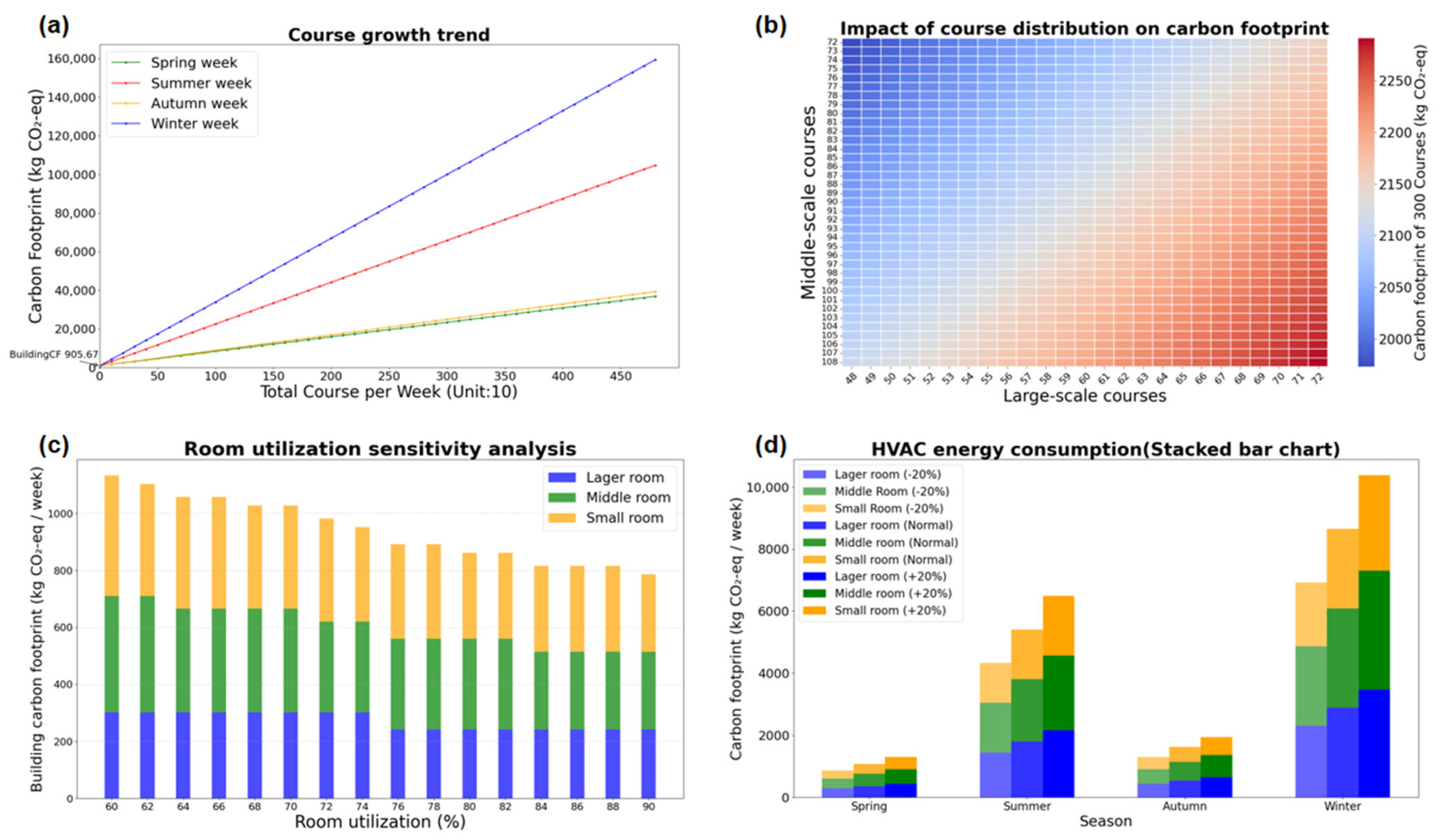
. The carbon footprint of the teaching activity under different parameters is analyzed to validate the applicability and comparability of the baseline strategy and optimization strategies. The sensitivity analysis results are shown in Figure 3.

Figure 3a illustrates how variations in the standard weekly course load (COURSE_WEEK) affect teaching activity’s carbon footprint across different seasons. The constant value of 905.67 kg CO₂-eq (standard week), marked as “BuildingCF” on the vertical axis, represents the weekly embodied carbon emissions from campus buildings, independent of scheduled teaching activities. The results show a near-linear response: a 10% increase in weekly course load leads to a 4.3% rise in emissions, while a 10% reduction results in a 3.8% decrease. The slopes vary by season, with higher increases in summer and winter, reflecting greater HVAC-related electricity demand associated with seasonal temperature differences. Figure 3b analyzes how different combinations of medium- and large-sized courses affect the standard weekly carbon footprint. The heatmap assumes a fixed total of 300 courses, with the number of small-sized courses implicitly being the remainder (i.e., 300 minus the sum of medium and large courses). The horizontal axis shows an increasing number of large courses from left to right, and the vertical axis shows an increasing number of medium courses from top to bottom. The color gradient from blue to red represents rising carbon emissions. A 10% increase in the proportion of large courses results in a 6.2% increase in electricity-related emissions due to the higher energy consumption of large classrooms. As more large and medium-sized courses are scheduled—shifting toward the bottom-right corner of the heatmap—the total footprint grows accordingly. This highlights that classroom size allocation significantly influences energy efficiency, and controlling the amount of high-energy course types can help to reduce electricity-related emissions under a fixed teaching load. Figure 3c illustrates how classroom utilization rates affect the total building-related carbon footprint under a fixed teaching load. In this strategy, the number of weekly courses is held constant at 300, and only the classroom usage arrangement is adjusted. The carbon footprint of buildings is treated as a variable, determined by the number of activated rooms required to meet the fixed schedule. A room is considered “in use” only if at least one class is scheduled within it during the week. As utilization rates increase from 60% to 90%, the same set of courses can be concentrated into fewer classrooms, reducing the number of buildings activated and thus lowering emissions. A 10% increase in utilization results in a 7.5% decrease in building-related emissions, while a 10% decrease leads to a 9.1% rise. Figure 3d shows how seasonal electricity consumption (ENERGY_SEASON) influences the weekly carbon footprint of teaching activities under different HVAC energy settings. The horizontal axis is divided into four seasons, and each season includes three stacked bars representing electricity consumption levels: a 20% reduction (left), the baseline level (center), and a 20% increase (right). Each bar is further segmented by color to reflect the contributions from small, medium, and large classrooms. The vertical axis indicates the weekly carbon emissions in kg CO₂-eq. The results reveal that changes in HVAC electricity consumption have a more pronounced effect in summer and winter, where a 20% increase leads to a 13.6% rise in emissions and a 20% reduction results in a 12.4% decrease. In spring and autumn, the overall changes are more modest, reflecting relatively lower HVAC usage in those periods. These findings indicate that HVAC energy optimization has greater potential to reduce carbon emissions during seasons with higher heating or cooling demands.

The detailed computational performance of the model—including the number of decision variables, constraints, solver time, and system specifications—is provided in Table S9 in Supporting Information.

The teaching activity carbon footprint in the baseline strategy consists of the building carbon footprint and electricity carbon footprint. According to the carbon footprint accounting results in Section 3.1, the annual building carbon emissions for large, medium, and small classrooms are fixed. 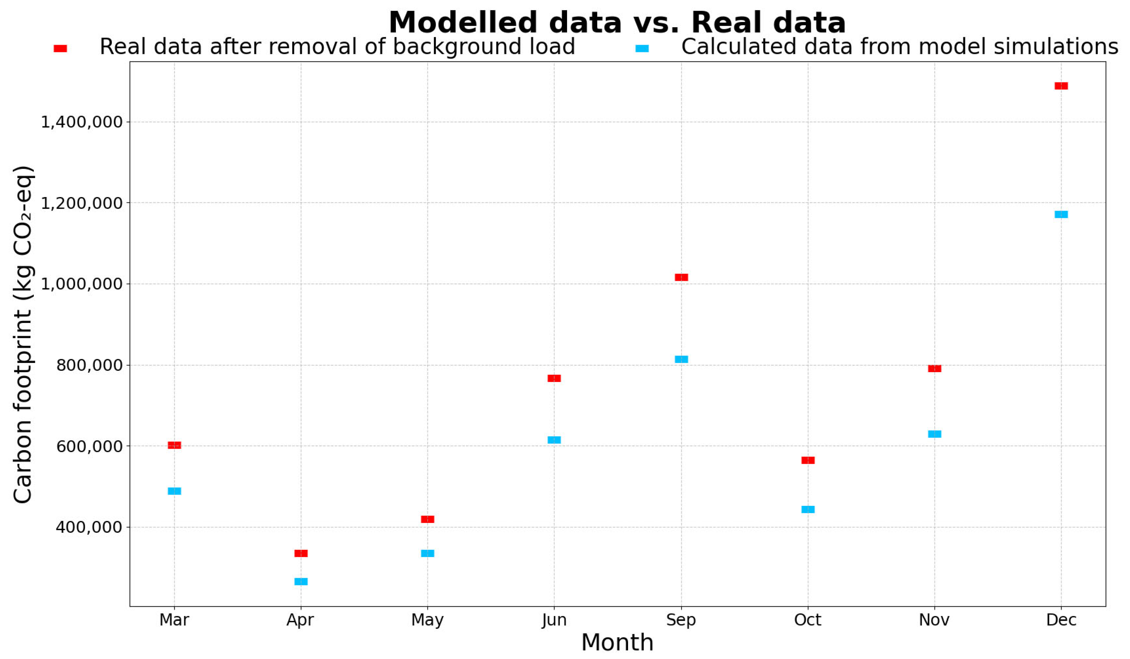Regardless of whether classrooms are in use, their carbon emissions are cumulatively accounted for, resulting in a total annual building carbon footprint of 723.68 t CO₂-eq for the university’s teaching buildings. The actual electricity consumption data for teaching months (excluding background loads) is compared with the modeled electricity consumption data for teaching months in the baseline strategy, as shown in Figure 4.

Regarding the university’s actual electricity carbon footprint data, electricity consumption is not solely attributed to teaching activities but also includes laboratories, infrastructure, administrative offices, and baseline energy loads from teaching buildings. Using electricity consumption data from non-teaching months (January, February, July, and August), the background load is estimated to account for approximately 34.7% of the total annual electricity consumption. This implies that 34.7% of the university’s total electricity consumption is used for laboratories, administrative buildings, and infrastructure. Teaching activities account for approximately 65.3% of total electricity consumption. The results indicate that the modeled trend in the energy-related carbon footprint matches the actual trend in electricity consumption after background loads are removed. The model particularly captures peak carbon footprint periods in June and December, demonstrating its effectiveness in accurately reflecting the contribution of teaching activities to carbon emissions.

The results of the sensitivity analysis and monthly simulation confirm the rationality and robustness of the teaching activity carbon footprint analysis model. The model demonstrates consistent and interpretable responses to parameter variations, and effectively captures the seasonal dynamics and structural characteristics of teaching-related emissions. Furthermore, the close alignment between the simulated outputs and the actual energy consumption trends supports the model’s applicability for campus-scale carbon accounting and optimization in subsequent sections.

3.3. Results and Analysis of Course Scheduling Optimization Strategies

By optimizing course scheduling strategies, this study examines the impact of Distributed PV Matching Optimization and Seasonal Energy Optimization on the carbon footprint of teaching activities and evaluates the potential emission reduction effects of Combined Optimization.

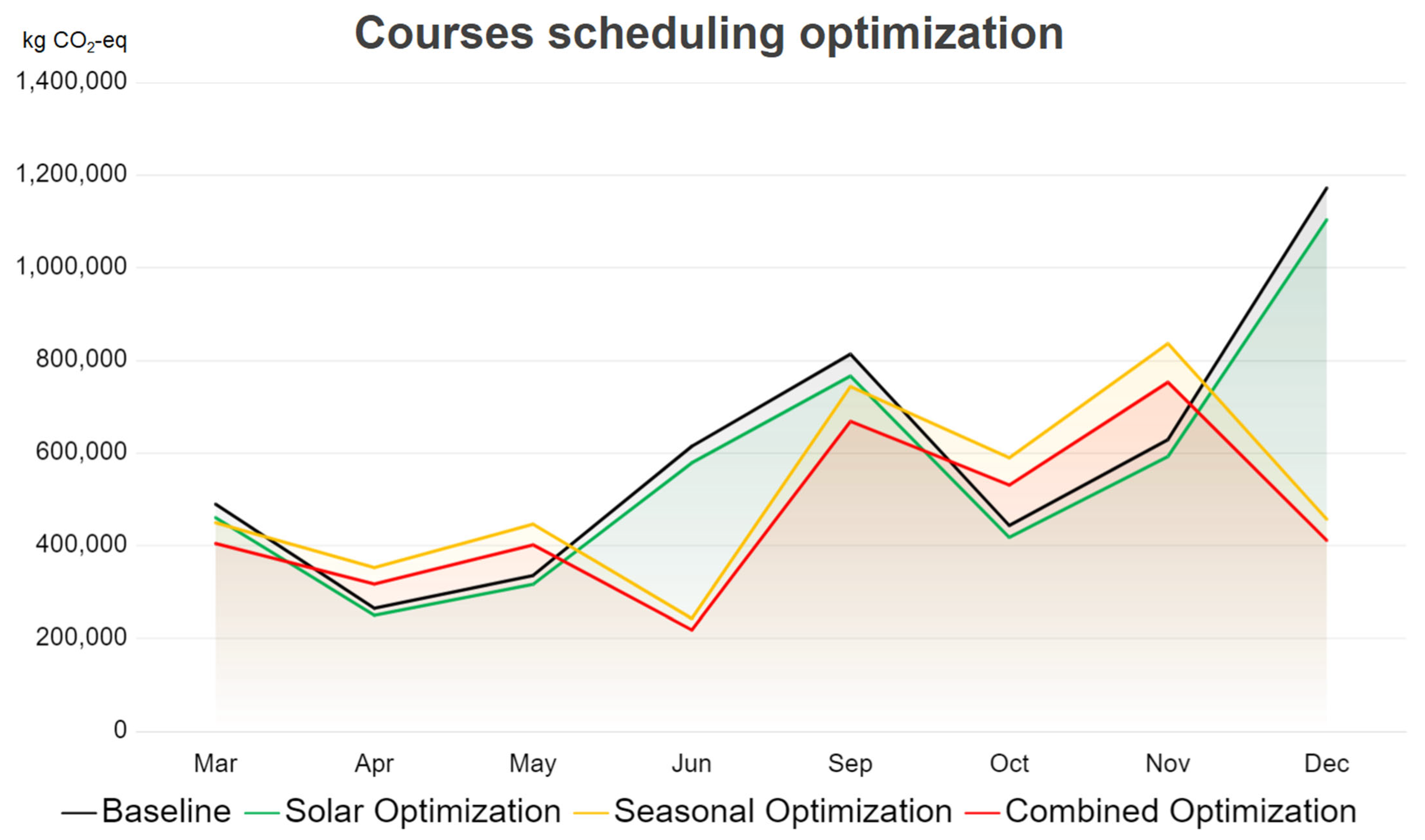
The carbon footprint optimization results for Distributed PV Matching Optimization, Seasonal Energy Optimization, and Combined Optimization under the Course Scheduling Optimization Strategy are shown in Figure 5.

When comparing the baseline scenario with Distributed PV Matching Optimization, the baseline features a relatively even distribution of course schedules, with over 30% of courses held at night, leading to higher electricity demand during non-PV generation hours (Figure 6, left). In contrast, under the Distributed PV Matching Optimization strategy (Figure 6, right), there is a significant shift in the spatial and temporal distribution of courses.

The results indicate the following improvements: Nighttime courses are reduced, with the proportion dropping below 20%, effectively reducing nighttime electricity loads. Daytime courses are more concentrated within high-efficiency PV generation hours (10:00–16:00), increasing their share from 58% to over 70%. This adjustment improves the utilization of self-generated PV power, reducing reliance on external electricity sources, and reduces the impact on the power grid by reducing online electricity through self-consumption. The results in Figure 6 show that Distributed PV Matching Optimization reduced annual teaching activity carbon emissions by 7% (approximately 333.31 t CO₂-eq) compared to the baseline strategy, though its standalone effect is limited.

In the comparison between the baseline and Seasonal Energy Optimization, the baseline strategy schedules a fixed number of 300 courses per week (COURSE_WEEK), maintaining a constant distribution regardless of seasonal variations. However, under the Seasonal Energy Optimization Strategy, the distribution of teaching activities is adjusted based on energy consumption patterns. During high-energy-consumption seasons (June and December), course loads are reduced by 30%, meaning that only 100 courses are scheduled per week, effectively reducing peak energy demand. During low-energy-consumption seasons (spring and autumn semesters), course loads increase to 400 courses per week, taking advantage of a more favorable energy environment and thereby improving the overall efficiency of course distribution. Seasonal Energy Optimization achieved a more significant reduction of 26.92% (approximately 1281.91 t CO₂-eq) compared to the baseline electricity consumption by adjusting course distribution to balance seasonal energy consumption.

Combined Optimization, integrating both strategies, resulted in a total annual carbon reduction of 45.95% (approximately 2188.13 t CO₂-eq). The synergistic effect of the Combined Optimization strategy allows for maximum PV utilization while optimizing seasonal teaching loads, making it the recommended low-carbon teaching scheduling strategy.

Prioritizing course scheduling during peak PV generation hours and reducing high-energy night courses enhance renewable energy utilization and lower reliance on purchased electricity. However, due to limited rooftop PV capacity at universities, the effectiveness of Distributed PV Matching Optimization depends on installed PV capacity and efficiency, making its carbon reduction impact relatively modest. Seasonal Energy Optimization achieves greater carbon reductions by reducing teaching loads during high-energy seasons (summer and winter) while redistributing courses to low-energy seasons, optimizing annual energy demand. The results suggest that Seasonal Energy Optimization is more effective than Distributed PV Matching Optimization when the renewable resources are limited, emphasizing the need for universities to consider seasonal energy load variations in teaching scheduling to avoid excessive demand concentration during high-energy periods. Further analysis reveals that single-timeframe optimization strategies yield limited emission reductions, whereas the combination of Distributed PV Matching and Seasonal Energy Optimization enhances overall carbon reduction efficiency. The Combined Optimization Strategy effectively reduces both daily electricity loads (Distributed PV Matching) and seasonal HVAC energy loads (Seasonal Energy adjustment), significantly lowering annual carbon emissions. This underscores that low-carbon teaching scheduling should adopt a multi-dimensional optimization approach rather than relying solely on time-based adjustments, maximizing carbon reduction potential.

3.4. Results and Analysis of Building Resource Optimization Strategy

New construction and campus expansion strategies are investigated to consider building resource optimization in order to adjust teaching space allocation and resource utilization. The New Construction with Optimized Utilization strategy assumes that teaching buildings have not yet been constructed, allowing for the optimal allocation of all teaching spaces while ensuring that course demands are met. The result comparison in the new construction context is presented in

Table 5. Comparison of baseline and optimized strategies in new construction context.

Strategy	Number of Courses per Week (Total)	Room Utilization	Number of Large Classrooms Required	Number of Middle Classrooms Required	Number of Small Classrooms Required	Total Number of Classrooms	Total Area of Teaching Buildings (m2)	Annual Building Carbon Emissions (t CO2-eq)
Baseline	unchanged	62.50%	45	75	120	240	64,500	725.88
New Construction	unchanged	90%	34	50	84	168	45,400	509.70

.

In the New Construction with Optimized Utilization strategy, the weekly course demand remains unchanged, but classroom allocation is optimized by increasing the utilization rate from 62.5% (baseline) to 90%. According to the scheduling model, this allows the required number of classrooms to be reduced from 240 to 168, including 34 large, 50 medium, and 84 small classrooms. As a result, the total teaching building area decreases from 64,500 m² to 45,400 m². Based on the daily carbon footprint factor of 0.030739 kg CO₂-eq/m²/day (Table S7 in Supporting Information), the annual embodied carbon footprint is reduced from 725.88 t CO₂-eq to 509.70 t CO₂-eq, representing a 29.8% reduction.

These findings demonstrate that the proposed scheduling and allocation algorithm can effectively reduce embodied carbon emissions during campus planning stages where spatial layouts are yet to be finalized. By identifying the minimum set of required classrooms under a fixed teaching demand and constrained utilization, the model supports spatially efficient planning and low-carbon construction decisions. This highlights the method’s applicability for greenfield development and new campus planning, where full flexibility in space design allows for significant carbon savings through optimized teaching space deployment.

In the Campus Expansion with Optimized Scheduling strategy, teaching activities increase by 50%, and spatial allocation is optimized to reduce additional construction needs. This strategy assumes that existing buildings remain unchanged and additional classrooms are added only as needed, with a maximum utilization rate of 90%. The results comparison under the campus expansion context is presented in

Table 6. Comparison of baseline and optimized strategies under campus expansion.

Strategy	Number of Courses per Week (Total)	Room Utilization	Number of Large Classrooms Required	Number of Middle Classrooms Required	Number of Small Classrooms Required	Total Number of Classrooms	Total Area of Teaching Buildings (m2)	Annual Building Carbon Emissions (t CO2-eq)
Baseline	Increase by 50%	62.50%	67	113	180	360	96,750	1085.51
New Construction	Increase by 50%	90%	50	75	125	250	67,500	757.33

.

Under the baseline expansion case, the total number of classrooms and the building area are increased proportionally to meet the additional demand at the original 62.5% utilization rate, resulting in 360 classrooms and 96,750 m² of teaching space. In contrast, the optimized strategy maintains a utilization rate of 90% and reallocates teaching schedules accordingly. This reduces the required number of classrooms to 250 and the total area to 67,500 m². As shown in Table 5, the annual building carbon emissions decrease from 1085.51 t CO₂-eq to 757.33 t CO₂-eq, achieving a 30.2% reduction despite the increased course volume.

In the context of campus expansion, where additional teaching facilities are needed due to increased demand, the model enables the refined estimation of spatial requirements without defaulting to linear proportional growth. Instead of expanding building capacity uniformly, the algorithm restructures course distribution to limit the number of new classrooms required, thereby avoiding unnecessary construction and associated emissions. This demonstrates the model’s value in retrofitting or partial expansion projects, supporting carbon-aware planning in existing educational infrastructures.

The results of both strategies confirm that the proposed scheduling-based optimization approach is adaptable to diverse campus development contexts. Whether in new campus planning or incremental expansion, the model provides a quantitative framework to guide teaching space allocation while minimizing associated carbon emissions. Its flexibility in handling fixed teaching loads, classroom utilization constraints, and varying spatial configurations makes it a valuable tool for carbon-informed educational infrastructure planning and long-term sustainability strategies.

4. Discussion

This study presents a framework for optimizing the carbon footprint of university teaching activities through detailed carbon accounting, dynamic activity modeling, and resource optimization. However, several limitations remain. First, our carbon footprint accounting relies on secondary data such as energy bills, equipment consumption databases, and literature-based building carbon intensity estimates, which may deviate from actual conditions. Specifically, the estimation of building material composition was based on the available literature due to the lack of detailed on-site data for the target campus. Future research may incorporate Building Information Modeling (BIM) or architectural design blueprints to refine material-level accuracy in carbon accounting. Moreover, the model does not fully capture the complexity of all teaching activities; for instance, the energy consumption of laboratory courses and online education [55] is not thoroughly considered. Additionally, our analysis is limited to optimizing classroom utilization and physical space expansion, without addressing renovation costs [56], construction timelines [57], or the acceptance of scheduling adjustments by faculty and students. Future research should incorporate behavioral data and additional operational constraints [58] to enhance the model’s practical applicability.

In addition to these limitations, several sources of model uncertainty should also be acknowledged. First, the carbon footprint factors used for electricity and building materials are based on national averages and literature-derived values, which may differ from localized or real-time conditions. Second, the assumed weekly teaching activity loads and classroom usage patterns are derived from typical scheduling profiles and do not reflect random fluctuations, emergency changes, or actual behavioral variations across departments. Third, the optimization process does not incorporate probabilistic uncertainty propagation or sensitivity analysis of key parameters (e.g., PV output variability, HVAC intensity), which may influence the robustness of the scheduling outcomes. Future work could integrate stochastic modeling techniques, parameter distributions, or Monte Carlo simulations to better assess the stability of optimization results under uncertainty.

Compared to existing studies that primarily rely on static accounting methods or focus narrowly on energy consumption metrics, this study introduces a dynamic framework that integrates life-cycle carbon footprint modeling with time- and capacity-based scheduling optimization. While prior works such as Helmers et al. [21,24] and Guerrieri et al. [20] offer valuable insights into university carbon footprint profiles and long-term transition paths, they lack the actionable modeling of operational-level scheduling activities. Furthermore, although studies like Wang et al. [23] explore the integration of PV generation and energy-saving technologies, their approaches do not fully incorporate dynamic teaching activity scheduling or infrastructure allocation constraints. On the other hand, optimization research in automated timetabling [29] excels at resource matching but often overlooks environmental impact considerations.

Our model contributes to bridging this gap by enabling integrated carbon reduction planning accounts for temporal, spatial, and infrastructure variables simultaneously. This framework is particularly applicable during planning or reorganization phases as this is when facility usage is flexible and emission structures are still malleable. Methodologically, the proposed MILP-based structure combines operational realism with life-cycle evaluation, offering a transferable template that can also be adapted to industrial production systems or urban infrastructure scheduling. By introducing carbon footprint awareness into scheduling algorithms, this work advances the theoretical foundation of operational-level decarbonization across domains.

Beyond the measures proposed in this study, further emission reduction strategies can enhance low-carbon campus operations. For example, rather than focusing solely on scheduling, AI techniques can be employed to reduce energy waste by automatically adjusting facilities [59] such as air conditioning [60] in unoccupied classrooms. Additionally, integrating expanded PV systems, distributed energy storage [61], and heat pump technologies for heating [62] can further lower carbon emissions. Encouraging low-carbon behaviors among students, such as waste sorting and reducing food waste, also plays a vital role in creating a more sustainable campus environment.

Although teaching activity scheduling is relatively straightforward, with fixed course loads and defined time slots, actual industrial production processes are far more complex. Industrial operations are influenced by intricate production mechanisms, order fulfillment requirements, and raw material supply constraints. Nevertheless, the modeling framework proposed in this study—combining life-cycle carbon accounting, spatiotemporal scheduling, and strategy-based optimization—offers a transferable methodological basis for broader applications. By adapting the input parameters and operational constraints to fit sector-specific characteristics, such as production lines or energy profiles, this approach can support proactive carbon mitigation in industrial parks, urban service systems, and other organization-scale operational settings. It thus contributes to the development of integrated carbon management systems that embed emission reduction strategies into everyday planning and operational decisions.

5. Conclusions

This study presents a comprehensive framework that integrates life-cycle carbon footprint evaluation with strategy-based scheduling optimization, addressing the persistent disconnection between carbon accounting and operational decision-making in general carbon management. By modeling the temporal and spatial dynamics of teaching activities, the proposed approach demonstrates how carbon emissions can be effectively minimized through strategic adjustments in schedule and resource allocation. The results highlight the importance of synchronizing academic operations with energy demand fluctuations and the availability of renewables, underscoring the role of institutional behavior in emission management. Furthermore, the study advances the system-level understanding of organizational carbon management by embedding emission factors into routine planning decisions, enabling a shift from post-evaluation to proactive mitigation. This integration of operational modeling with carbon accounting not only provides a practical tool for optimizing campus systems but also yields a scalable paradigm for application in broader regional or institutional carbon governance. It contributes to the theoretical development of low-carbon management strategies and supports long-term decision-making in energy-intensive operational environments.