Article

Empirical Insights into Economic Viability: Integrating Bitcoin Mining with Biorefineries Using a Stochastic Model

1
Faculty of Science and Technology, University of Stavanger, 4036 Stavanger, Norway
2
Department of Economics, Yıldız Technical University, Istanbul 34220, Turkey
3
School of Civil and Environmental Engineering, Yonsei University, Seoul 03722, Republic of Korea
*
Author to whom correspondence should be addressed.
Systems 2025, 13(5), 359; https://doi.org/10.3390/systems13050359
Submission received: 3 April 2025 / Revised: 2 May 2025 / Accepted: 5 May 2025 / Published: 7 May 2025

Abstract

:
This study explores integrating Bitcoin mining with lignocellulosic biorefineries to create an additional revenue stream. Profits from mining can help offset internal costs, reduce business expenses, or lower consumer prices. Using sensitivity analysis and Monte Carlo simulations, this study identifies key profitability drivers, such as electricity costs, hardware expenses, starting year, and operational time. Time emerged as an extremely sensitive factor and showed that delaying mining operations significantly raised production costs and the probability of profitable outcomes. In contrast, longer mining durations had a smaller yet sizable impact. Hardware costs, computational efficiency, and electricity prices also strongly influenced the outcomes. The majority of simulated events showed a loss. Moreover, the model showed that the marginal profitability of mining decreases over time. Nonetheless, the model demonstrated that under favourable conditions, it is possible to integrate Bitcoin mining into biorefineries and other productive ventures, thereby allowing for cost recovery using Bitcoin profits. For a biorefinery to mine Bitcoin and maximise cost recovery, it must start early, access low electricity prices, and preserve hardware capital characterised by low expenditure and high revenues. Finally, a discussion about the opportunities, risks, and regulations is highlighted.

1. Introduction

Lignocellulosic biomass (LCB) is a globally abundant and distributed natural resource. This includes, but is not limited to, agricultural wastes, agro-industrial processing wastes, forestry wastes, energy crops, and non-food crops [1]. Due to its characteristically high carbon density, LCB is considered to be a suitable feedstock for a variety of industrial applications. LCB feedstocks can be converted to value-added products (VAPs) and/or bioenergy for further utilisation. Current estimates suggest global LCB production capacities range between 180 and 200 gigatons per annum, of which only ≈5% is upcycled and productively used in a biobased value chain [2,3]. Moreover, it is also estimated that ≈80 Mt of LCB is needed to produce 30% of the biobased products, power, and heat in the European Union by 2030 [4]. An integrated lignocellulosic biorefinery (IB) employs various process conversion technologies, preferably creating biofuel and biochemical VAPs in tandem, as opposed to a single process with limited product scope and low reintegration capabilities.
VAPs generated through biomass refining are costly and less competitive as opposed to their more traditional petroleum-based counterparts. Biorefineries still experience commercialisation issues regarding pretreatment strategies, increased energy demands, and enzyme and feedstock costs, amongst others [5,6]. Even though IBs are capable of producing important VAPs (e.g., biofuels, lactic acid, ethanol, phenolics, resins, and more), they face difficulties doing so profitably, which render LCB underutilised due to high onset costs. Rather than landfilling or openly combusting LCB, which leads to unintended environmental issues, systematic innovations in IB design and operations are needed to overcome current bottlenecks. Although IBs have significant commercial potential, they must generate positive net returns to attract and sustain business investment. The financial obligation of an IB is to be and remain profitable, in order to continually offer its products and services [7]. When costs continually outweigh revenues, then inevitably, at some particular point in the future, the business venture collapses. In any biorefinery, technical process efficiencies, product yields, and chemical costs are critical factors to optimise as they affect bioproduction and economic potential [8]. Process integration and economies of scale are also important factors to consider [9]. For example, enhanced lignin extraction and its utilisation within other biobased VAPs is one of the ways to accelerate biorefinery integration and circularity, as well as improve economic conditions [8,10]. It has been shown that lignin removal and reintegration as a VAP can decrease the minimum selling price (MSP) of biofuels by ≈17.5 to 24.3%, depending on the treatment used [11]. Similarly, the production of phenolic compounds after removing lignin showed an overall decrease in the MSP from USD 2.09 to USD 1.94 per gallon of ethanol as lignin use increased from 30 to 90% [12], with desirable increases in the internal rate of return (IRR) and return on investment (ROI). Other researchers show similarly encouraging biorefinery economics as a result of process integration and co-product generation [13,14,15].
Bitcoin is a peer-to-peer digital timestamping protocol [16], and its native token, BTC, is the most widely adopted and most liquid cryptocurrency. Bitcoin has the largest market capitalisation and a fixed supply schedule, thereby making it an attractive candidate for financial and industrial integration [17]. Different economic theories consider how digital forms of money, like Bitcoin, relate to state intervention and market-driven approaches [18]. Interest in both Bitcoin as an asset and in mining as a revenue source has been increasing. Traditional energy companies, such as ExxonMobil and ConocoPhillips, are investigating Bitcoin mining using flare gas [19]. Other industrial players, such as Vespene Energy, Argo Blockchain, and Hive Blockchain Technologies, are using cheap or otherwise abandoned energy sources such as landfill CH4 [20], and hydroelectric and geothermal power to mine Bitcoin [21]. Moreover, established asset management firms, such as Fidelity and BlackRock, have also taken an interest in the digital asset [22] and are shareholders in Bitcoin mining companies. Recently, Bitcoin mining using geothermal energy has shown promising results with a positive NPV of USD 113.2 × 10⁶ and IRR of 47.3% [21]. The authors also showed a substantial decrease in the payback period as a function of the number of BTC mined as well as the BTC market price.
Through various biochemical, thermochemical, or combined conversion routes, LCB can be used to generate fuel and thus, electricity [23]. A specific amount of biofuel embeds within it a particular amount of energy. The combustion of a generic biofuel CaHbOc yields a specific amount of energy, as given in Equation (1). Energy conversion efficiency varies depending on the type of biofuel and the power generation technology used [24]. For example, fuel cell technologies, on average, have higher electrical generation efficiencies, ranging from 30 to 40%, as opposed to internal combustion engines. If cogeneration configurations with heat recovery units are used, the overall efficiency can rise up to 90% [24]. Therefore, an IB producing higher energy-rich biofuels and maximising energy conversion will result in higher electrical power output, where power output is a function of the efficiency of the energy conversion process. Therefore, in the context of Bitcoin mining, miner productivity is a function of the biofuel used, energy conversion system chosen, and power and electricity generated, as well as mining machine specifications. IBs have access to on-site-generated fuels as one of their products generated during the conversion process, which, if conditions such as IB size, costs, location, and others are favourable, can be leveraged to produce electricity and mine Bitcoin using scale-suitable data centres. However, the authors do not endorse or support the usage of first-generation biomass sources to fuel Bitcoin mining ventures. Nevertheless, inexpensive or excess energy and heat stemming from second-, third-, or even fourth-generation biofuels can be put to more productive uses through mining, if it is viable. For example, it was shown that syngas (19 MJ/kg) is only capable of producing 537 sats/kg, while bioethanol (29.8 MJ/kg) produces 877 sats/kg [25], where 108 sats = 1 BTC. Biohydrogen (141.8 MJ/kg) is capable of generating 3904 sats/kg. For instance, using biohydrogen and the S19 XP miner can produce 2905 sats/kg, whereas only 1388 sats/kg can be produced with the S17 miner [25]. Similarly, more energy-efficient and cost-effective hardware displaces less efficient and more expensive alternatives [26]. The S21 Hydro (335 TH/s—5360 W) offers a 34% increase in mining returns compared to the older S17 models (53TH/s—2385 W). For example, 1 kg of bioethanol (HHV = 29.8 MJ/kg), when converted to electricity via an internal combustion engine operating at 30% efficiency (ηe), yields 2.25 kWh, generating approximately 0.19 USD/kg, assuming an electricity price of 85 USD/MWh. Alternatively, utilising the same quantity of fuel to mine Bitcoin with an Antminer S19 XP (21.5 J/TH) produces 653 sats/kg (at 600 EH/s), corresponding to approximately 0.65 USD/kg at a Bitcoin price of USD 100,000, thus achieving a gross revenue approximately 3.5 times higher.
C a H b O c + a + b 4 c 2 O 2 a C O 2 + b 2 H 2 O + H e a t ( Δ H < 0 )
While there are criticisms regarding the environmental impact, electricity consumption, and reliance on fossil fuels associated with Bitcoin mining, several studies have increasingly highlighted its potential to support sustainable energy transitions and contribute to the UN Sustainable Development Goals (UN SDGs) [19,20,27,28,29,30,31]. Bitcoin mining’s unique ability to act as a flexible, interruptible energy consumer allows it to stabilise grids with high renewable penetration by absorbing excess electricity during off-peak periods [19]. Companies like Vespene Energy and Crusoe Energy are increasingly utilising stranded or wasted energy like flared CH4 or landfill CH4, which is over 80 times more potent than CO2, thereby reducing emissions while generating economic returns [19]. Moreover, the co-location of mining activities around renewable energy sources is incentivising the capacity buildout for these energy sources, thereby supporting the ESG framework [27,32]. On-site fuel use can reduce overall emissions by minimising transport-related losses and allowing better emission control through centralised combustion. Finally, while currently, the majority of mining operations use fossil fuels, a trend in recent years has shown that renewables and nuclear energy are being added into the electrical mix in larger portions [19]. For example, IREN Ltd. (Australia) completely powers all of its facilities with renewable energy.
Integrating Bitcoin mining operations into biorefineries is a novel proposal that warrants further study. The core hypothesis is that revenue from mining, whether through the use of internally produced biofuels or purchased electricity, combined with potential Bitcoin price appreciation, could indirectly subsidise biorefinery operations by offsetting biochemical production costs. Industrial players are able to turn energy production into an extra passive side stream of future deferred revenues [25]. IBs can leverage this additional revenue stream to support internal cost reductions, business expansions, or lower VAP pricing for consumers. Concretely, if mining profits cover a percentage of the fixed and variable costs, an IB can lower the sales price of key VAPs by equivalent percentages, all while remaining profitable and enhancing their own market competitiveness. While advances have been made in other industries and sectors by incorporating Bitcoin mining [19,33,34,35,36,37], there is a lack of research pertaining to assessing the inclusion of Bitcoin mining in IBs to improve their overall economic viability and cost efficiency. In this study, we address that gap by investigating whether and under what conditions an IB can economically benefit from housing Bitcoin mining operations. This study aims to develop a stochastic base model to calculate the minimum profitable mining price, which can be further used to assess viability of co-integrating Bitcoin mining operations into IBs. Through sensitivity analyses and uncertainty simulations, we identify key drivers of profitability for this integrated system. This integration leverages the IB’s abundant low-cost (or excess) bioenergy to run Bitcoin mining on-site. By using fuel that would otherwise be wasted or sold at low margin, an IB generates extra revenue that can offset operational costs, thus enhancing economic viability [25]. Moreover, this article aims to establish the case for and encourage the acceleration of additional research aimed at investigating Bitcoin mining in relation to the production of cheaper and more sustainable biobased products and energy from IBs. The proposed model biorefinery is given in Figure 1.

2. Bitcoin Mining: Technical Background and Economic Rationale

To understand the practical requirements of integrating mining into IBs, it is important to explore how Bitcoin mining works on a technical level. Briefly, Bitcoin miners solve cryptographic hashing puzzles to earn the right to add the next block to the blockchain. Application-specific integrated circuits (ASICs), known as miners, are specialised hardware designed to perform rapid iterations to find a number, called a nonce, that meets a changing set of criteria set by the Bitcoin network. This process involves trial and error, as ASICs choose a nonce, attach it to the current block, and hash the data using the SHA-256 algorithm. The goal is to produce an output hash smaller than a target number determined by the network’s difficulty level. Once a nonce is found that satisfies the conditions of a valid block, the solution is broadcast for verification, and the miner earns newly mined BTC and transaction fees for the block. This process repeats approximately every 10 min. Every 2016 blocks (roughly two weeks), the difficulty adjusts based on the network’s total hashrate, maintaining a consistent 10 min block time. Every 210,000 blocks, the protocol cuts the block reward in half. If BTC’s value goes up or electricity becomes cheaper, more computational power is used. If BTC’s value drops or electricity becomes more expensive, less computational power is used. Over time, the total hashrate is proportional to the value of Bitcoin relative to the electricity price denominated in BTC terms [26]. Miners with lower costs will naturally displace those with higher costs, as the addition of hash power by profitable miners reduces marginal profitability. Bitcoin, unlike other energy-intensive systems and networks, does not aim for a fixed amount of energy use. Instead, it targets a specific block time and adjusts the amount of hashes needed by modifying the difficulty parameter every 2016 blocks, thereby balancing the network to achieve this intended energy expenditure [26]. The difficulty adjustment calibrates the network such that the amount of computational work being performed adjusts based on the economic conditions. The process has been described in more detail elsewhere [16,38]. According to the network parameters, only 21 million BTC will be mined, of which 93% have already been produced. The last BTC will be mined in the year 2140.
In this decentralised network, nodes participate in validating and propagating transactions into blocks through intensive computational effort. By employing a (Proof-of-Work) PoW consensus mechanism, miners are able to contribute computational power and participate in keeping the Bitcoin network secure, thereby eliminating central points of failure and centralised network control [16,39]. The PoW consensus mechanism ensures that mining requires energy in the form of electricity to keep the blockchain secure. For their work, miners are awarded virtual spendable BTC coins, whose value crossed over USD 100,000 in December 2024.
PoW ensures that the Bitcoin network experiences rising costs of production over time due to increasing mining difficulty [40]. This ensures BTC’s scarcity and value proposition over time, similar to the rising costs of production in traditional commodities relative to remaining supply. This rising cost of production reinforces BTC’s long-term value by providing support to market prices, enhancing network security, preventing central points of failure, incentivising investment, and driving forward energy efficiency. If BTC fills the role of store of value [41], the question then becomes, how can IBs participate and benefit from that? In some cases, it may not be profitable to undertake such a venture. Forecasting profitability and cost recovery is essential in prudent financial planning for assessing long-term viability [42]. The process is dependent on a multitude of factors ranging from IB design and size to biofuel production capacity, mining efficiency, electrical services expenses, BTC network state, BTC market price, governmental regulations, and public instruments, all of which influence an IB’s ability to recover costs.

3. Methodology

A stochastic financial model was developed to evaluate the potentiality of adding Bitcoin mining to IB operations as an adjunct revenue stream. The model was designed to determine the conditions under which mining becomes profitable and to quantify the effect of various internal and external factors on profitability. In particular, it forecasts two key outputs. First, the minimum profitable mining price (PP), which is the IB-specific cost of mining and can differ between ventures, and second, the profitability criterion (PC) that benchmarks the mining performance against forecasted Bitcoin prices.

3.1. Minimum Profitable Mining Price and Profitability Criterion

Bitcoin mining, under favourable conditions, could act as a subsidy to an IB. It could minimise the payback period, bring down costs, generate an added revenue, improve profitability, and reduce the required sale price of VAPs, making the IB’s overall operations more competitive. However, valuing BTC and the network through traditional capital budgeting techniques is not possible because BTC, in and of itself, does not generate a cash flow or yield. Therefore, asset-based, market-based, or comparative valuations must be used to better understand the integration of Bitcoin mining into IBs.
The model tracks a number of variables that describe the IB mining setup, costs, and the evolving Bitcoin network conditions, as well as evolving IB conditions.
The model equations are formulated in yearly intervals, with various time notations used to capture the temporal dynamics of BTC mining operations within an IB. The variable i denotes the initial year that the IB mining operation is chosen to start and is measured as the number of years since the Bitcoin genesis block (3 January 2009). For example, in this current year, i = 16 since it is the 16th year since the genesis block. The planned duration of IB mining activities is represented by T years. The variable τ is chosen to denote the number of 4-year epochs within T. For example, if T = 22 years of mining operations, then the IB would experience five 4-year epochs in 20 years, with 2 remaining years. This provides the flexibility to start the analysis at any year within a Bitcoin halving epoch without having to start and stop operations in complete epoch periods and enables a more detailed and precise representation of revenues. Setting up the model equations in this manner also accommodates the strategic planning and analysis of IB mining operations that closely align with the halving schedule, thus offering a more comprehensive view of potential profitability across varying market conditions and operational timelines. Moreover, the general time variable used in the equations is given as t. To generalise the model across arbitrary start times (i) and lengths (T), time is normalised such that t = i denotes the first year of mining operations (i.e., ti = 0 in model terms). Thereafter, the model equations are assessed from t = i to t = i + T at the boundaries, enabling the model to take T and i as inputs. Finally, the mapping function h(t) maps t onto discrete intervals that are multiples of 4, starting from i. This ensures that, whenever needed, t jumps in steps of 4 units, effectively creating a series of discrete time points (i.e., h(t) = i, i + 4, i + 8, …). Therefore, h(t) mitigates time-dependent changes in situations where model parameters are expected to remain constant for that specific period, where others are changing. For example, such situations arise when using the same specification of ASIC miners for a 4-year period. Since variables such as nt, HM, εM, and CM are derived yearly, h(t) ensures that whenever needed, changes within calculations are considered every halving epoch instead of yearly.
t = t i m e , i n   y e a r s , s i n c e   t h e   g e n e s i s   b l o c k   ( 3   J a n u a r y   2009 )
h t = i + 4 · t i 4
h i = i
h τ = i + 4 · τ
τ = t i 4 such   that   t 4 τ + i , 4 τ + 4 + i
The number of ASIC mining machines in any operational year t is given as nt, with the initial fleet size being n0. In terms of the number of ASICs, nt is allowed to grow or decline over time to reflect hardware additions or retirements. The inter-epoch growth and decay rates in the number of ASICs are given as gM and dM. The fraction of capital expenditure, ECAP, assigned to the initial installation and infrastructure at t = i is denoted as θINS and θINF (e.g., site preparation, electrical and networking setup, labour for deployment). Subsequent installations and infrastructure upgrades are given as ρINS and ρINF, respectively. Each ASIC unit has a purchase cost CM (USD) and delivers a certain hashrate HM (terahash per second, TH/s) with a given power efficiency εM (J/TH). The ASIC cost of computation is given as PM (USD/TH/s). A depreciation rate, δM, is included to account for the loss in value of ASIC hardware over time. Usually, ASICs are assumed to depreciate in a straight line down to USD 0 over the useful lifetime. However, logically, ASICs that are no longer profitable under a certain condition can still make use of geographical arbitrage and be moved to areas with a lower cost, thereby allowing them to become profitable again. Bitcoin mining provides a flexible, interruptible power sink that turns curtailed or stranded renewable electricity into profit, acting as buyers of last resort without increasing electricity prices [19]. Therefore, the salvage value of used ASICs is always greater than and never USD 0 because ASICs are always profitable elsewhere. ξM denotes the bulk discount/coupons on ASIC purchases. Additionally, CELE is the cost of electricity, which, in the context of an IB, is interpreted as its own levelized cost of electricity (LCOE) for power either generated on-site from the IB’s biofuel or by purchasing electricity from the grid, either directly or through a power purchasing agreement. Because CELE is essentially an already discounted metric, when it is included in the yearly EOP, it is not discounted again. It is important to note that the calculation of CELE itself contains significant variations and uncertainties, which are dependent on scale, location, fuel type, and other factors, such as technology efficiency, capital costs, and regulatory environment. Connection to cheaper power generation sources, such as combined-cycle gas turbines, geothermal vents, and ocean thermal energy conversion (OTEC), warrants further investigation under the proposed model. Finally, annual maintenance costs (repairs and upkeep of mining equipment) are given as σMT, and σIB is assigned to IB-specific costs related to BTC mining itself and not costs related to biorefinery activities.
Moreover, several variables capture the state of the Bitcoin network and mining rules, as these external factors heavily influence an IB’s success in mining BTC. The total network hashrate at time t, given as HN,t, is the global computational power of all Bitcoin miners combined. From an IB’s perspective, HN,t is a dynamic, exogenous variable that HM,t is a fraction of. Mining rewards come from two sources. First, miners earn the block subsidy, which is the new BTC mined with each block, given as ϕ. The block subsidy is an exogenous variable and halves every 210,000 blocks (≈10 min per block, approximating 4 years). The initial block subsidy in 2009 was ϕ0 = 50 BTC and, thereby, was cut in half over successive epochs. The model accounts for ϕ halving changes over time. Second, miners earn transaction fees within a block, denoted as ω. A general upward trend in fees over the long term is assumed, especially as block subsidy is diminished. The growth rate in fees over time is denoted as gFEE. BTC rewards are both fixed in time and proportional to the amount of hashing power (PoW) contributed. Therefore, the probability of a miner finding a block is taken to be the ratio of their hashrate to the total network hashrate, whilst also accounting for when the IB begins mining operations (i.e., what the block reward is at t = i and going forward). The number of blocks mined per year is given as βt. Also, the model includes a variable for mining pool fees in exchange for more steady income, given as α. Finally, the forecasted price of BTC at time t is given as PBTC,t. The list of model equation variables is given in Table 1.
The model outlines an IB’s mining venture over a period of years and tallies all associated costs and revenues. Equations (7)–(11) form the core of the model and are used to calculate PP and PC, which are decision-based metrics that inform an IB as to their costs and revenues associated with integrating mining operations. The core equations are structured to ensure the total costs forecasted over time accurately reflect future changes an IB undertakes, such as upgrading ASICs to increase their HM in response to changing HN. Similarly, the total projected revenues over time must reflect changes the Bitcoin network imposed on participants, such as generally increasing HN and decreasing ϕ, as well as global ASIC efficiency improvements. The equations are as follows. Equation (7) gives the minimum profitable mining price (the IB’s lowest cost of production achievable). Equation (8) gives the operational expenditure, EOP, over the mining duration of T years. Equation (9) gives the total BTC revenue produced, RTOT, that an IB would earn from mining between year i and year i + T. Equation (10) gives the profitability criterion, PC, defined as the ratio between PP and a forecasted spot price, PBTC,t. A value of PC below 1 indicates the mining operation would be profitable, whereas a value of PC above 1 signifies an unprofitable scenario. Equation (11) represents the necessary capital expenditure, ECAP, over the project lifetime T years. Finally, all forecasted costs and revenues in the model are treated in present value terms using a discount rate r, except when noted otherwise.
Equation (11) lays out the ECAP costs associated with initiating and maintaining an IB mining project. This encapsulates the costs of purchasing and upgrading ASIC hardware as well as improving the associated infrastructure over time. The structure of Equation (11) is given in such a way in order to dynamically handle both complete (T is a multiple of 4) and incomplete epochs (T is not a multiple of 4) since the Bitcoin halving occurs every 210,000 blocks ≈ 4 years. ECAP is composed of 7 terms, A through G, given as Equations (12)–(18).
First, term A captures the installation and infrastructure buildout of IB mining facilities at the beginning of operations, where t = i. The installation and infrastructure costs are parametrised as θINS and θINF, respectively, and are assumed to scale with the size of the initial ASIC deployment. Second, term B deals with subsequent installation and infrastructure upgrades brought about by the increase in the IB’s total hashrate increase. Such upgrades occur at the start of every epoch τ. These future costs are discounted to their present value. Third, terms C, D, and E deal with the acquisition and resale of depreciated ASICs across T to maintain competitiveness. Term C covers the initial purchase of ASICs at the beginning of operations, where t = i. Term D represents the cost of periodic ASIC upgrades at each epoch, as well as the resale value from replacing hardware. Term E deals with the sale of depreciated ASIC capital at the end of the last epoch. In both terms D and E, future costs and recovered revenues are discounted to their present value. Finally, terms F and G are included to handle cases where the IB’s chosen mining period T does not align exactly with the end of a four-year halving cycle. When T is a multiple of 4, terms F and G cancel each other. However, if T includes a partial epoch, terms F and G do not cancel, which ensures the costs and sales of depreciated ASIC assets are accounted for appropriately in this last partial cycle. Here, future costs and revenues are also discounted to their present value using r. By structuring ECAP in this manner, the model equations can accommodate any mining duration T, aligning capital investments and salvage values correctly with the Bitcoin halving schedule.
P P = C T O T R T O T = E C A P + E O P R T O T
E O P = t = i T + i n t · H M , h ( t ) · ε M , h ( t ) · C E L E + t = i T + i n t · σ M T + σ I B ( 1 + r ) t i
R T O T = t = i T + i n t · H M , h ( t ) H N , t · ϕ 0 · 1 2 t 4   + ω · 1 + g F E E t i · 1 α · β t
P C ( t ) = P P ( t ) n B T C t · P B T C ( t ) f o r   a l l   t T   i s < 1 ,       p r o f i t a b l e = 1 ,       b r e a k e v e n > 1 ,       u n p r o f i t a b l e
E C A P = A + B + C + D E + F G
A = n 0 · C M , h ( i ) · ( 1 ξ M ) · θ I N F + θ I N S
B = τ = 1 T 4 n τ · C M , h ( τ ) · ( 1 ξ M ) · ρ I N F + ρ I N S 1 + r 4 τ
C = n 0 · C M , h i · 1 ξ M
D = τ = 1 T 4 1 n τ · C M , h ( τ ) · ( 1 ξ M ) 1 + r 4 τ n τ · C M , h ( τ ) · ( 1 ξ M ) · 1 4 · δ M 1 + r 4 τ + 4
E = n T / 4 · C M , h ( T / 4 ) · ( 1 ξ M ) · 1 4 · δ M 1 + r 4 T 4
F = n T / 4 · C M , h ( T / 4 ) · ( 1 ξ M ) 1 + r 4 T 4
G = n T / 4 · C M , h ( T / 4 ) · ( 1 ξ M ) · 1 δ M · T 4 T 4 1 + r T
The model Equations (7)–(11) were used to determine the costs and benefits associated with adding Bitcoin mining to an IB. It is important to emphasise that this analysis focuses solely on the aspect of integrating mining operations with an IB with costs and revenues pertaining to that integration only (i.e., it applies exclusively to expenses associated with Bitcoin mining that an IB has to finance and not to the costs of building and operating the IB itself). Should one choose to incorporate the capital and operational expenditure of the IB itself, it is imperative to concurrently consider IB revenues and conduct that analysis in conjunction. However, such an analysis exceeds the scope of this study, as it primarily focuses on the Bitcoin mining segment within an IB.
Finally, to evaluate model outcomes, a sensitivity analysis was conducted by varying individual parameters ±50% from their baseline values and observing changes in PP. This included one-at-a-time variations and pairwise heatmaps to assess interactive effects, as given in Figure 2 and Figure 3. A Monte Carlo simulation was then performed using the probabilistic distributions for key variables in Table 1, producing a distribution of profitability outcomes for PC. Monte Carlo analyses were conducted using 2 to 4 million simulations, which was enough to achieve convergence and stability in the output distributions. The results from the Monte Carlo simulations are given in Figure 4, Figure 5 and Figure 6. The analyses were conducted in Microsoft Excel.

3.2. Model Assumptions and Key Details

The following assumptions were made to simplify model calculations. It is imperative to delineate these assumptions and nuances explicitly, as they influence the variables within the model equations, consequently impacting the resulting outcomes.
First, the model assumed that all variables remain constant within each simulated one-year interval. In practice, the network hashrate, number of active ASIC machines, fees per block, BTC price, and others, change continuously. However, such values are assumed to be constant for the specific year period and only updated at the end of each year t.
Second, ASIC miners were assumed to operate at 100% uptime, running continuously throughout the year without scheduled or unscheduled downtime due to maintenance or utilising the flexibility in mining (i.e., turning ASICs off to utilise electric power elsewhere). Operational surveys indicate fleet-wide uptimes of roughly 98% [43]. During these short outages, miners commonly deploy autotuning overclocking firmware on the remaining units to compensate for HM,t. Practitioners may, therefore, scale HM,t by an availability factor (e.g., 0.98) to incorporate site-specific downtime. It is important to note that an ASIC that is not running does not generate any revenue, but, at the same time, it does not incur any costs, aside from procurement and storage costs.
Third, it was assumed that the number of blocks per year was 52,500 (i.e., 210,000/4 years). However, since Bitcoin operates using block height as its reference in time, the time needed to produce 210,000 blocks is always slightly less or more than 4 years. Roughly 4 years is targeted by adjusting the mining difficulty every 2016 blocks to satisfy the rule of 1 block every 10 min.
Fourth, the model represented the growth in the IB’s ASIC fleet in discrete four-year intervals, aligned with Bitcoin’s halving epochs. At the start of each epoch, the number of ASIC units was increased by a growth factor gM to enhance HM. A decay factor dM was applied to moderate this growth over time, reflecting diminishing operational size as the time increases. The number of ASICs at any time t is given as Equation (19). The initial number of ASICs, n0 at t = i, is chosen by the IB and is a function of the size of the operation and available power, as well as their funding capacity. This structure captures the strategic necessity of continuous hardware investment in response to ϕ decreasing, and HN generally increases over time.
n t = n 0 · 1 + g M · 1 1 + d M · t i 4 t i 4
Fifth, the total network hashrate at any time t, HN,t, was the total sum of all computations on the network. HN,t is a dynamic network variable that is out of the control of any single user, thereby making forecasting challenging and speculative. The model equations are modular, such that the user can specify various projections and scenarios for HN,t. In this case, a power-law growth trend was assumed to forecast HN,t based on historical data regression. The data spanned the daily network hashrate between 1 January 2010 and 26 April 2024 (R2 = 0.975), given as Equation (20). Due to the power-law fitting, it was assumed that HN,t keeps rising; however, this may not be true in reality.
l o g 10 ( H N , t ) = 4.7161 + 11.997 · l o g 10 t ; R 2 = 0.975
Sixth, while ϕ can be deterministically determined beforehand, ω may vary widely between blocks. Assuming ω to be a static fraction is incorrect since fees vary with time in no predetermined fashion. Over a longer period, however, it is expected that ω eventually rises to compensate miners for the decrease in ϕ. At any given moment, the variability in ω is naturally quite large, with values varying by 100-fold or more, with observed ranges spanning between 0.003 and 9.67 BTC/block. The Bitcoin transactional blockspace is limited in size, and over the long term, block production becomes solely a function of time. Currently, ω in most blocks does not exceed ϕ; however, they are expected to grow and become the primary revenue source for miners. This transition would occur over many years as demand for blockspace increases, pushing fees higher. Over time, the percentage of revenue stemming from fees (i.e., ω/ω+ϕ) trends towards 100% as ϕ asymptotically decreases to 0. With the fee spike of April 2024, this ratio reached above 75% for the first time but has since fallen back down to ≈1%. This makes forecasting ω highly uncertain. With that being said, any ϕ or ω in absolute terms is sufficient, as long as PBTC,t remains sufficiently high enough to cover operational expenses and still yield a marginal profit for the IB. Therefore, the initial value of ω taken was simply the average fee per block aggregated from 1 January 2012 to 22 April 2024. The average fee calculated was 0.4323 BTC/block. A fee growth rate, gFEE, was also assumed.
Seventh, the model accounted for the likelihood that future ASIC hardware will be more powerful and energy-efficient. The hashrate and power efficiency, HM and εM, of future ASIC models were based on empirical assessments with historical ASIC data fit to a power law from June 2016 to April 2024, with R2 = 0.859 and 0.917, respectively. εM (J/TH) inversely affects operational costs. Higher-efficiency ASICs (i.e., lower J/TH) imply lower energy costs for the same hashrate over time. Therefore, it is imperative that an IB increases their deployed computational power over time using more efficient ASICs to keep up with changes in HN,t. HM,t is given as Equations (21) and (22), whereas εM,t is given as Equations (23) and (24). In the current assumption, it was assumed that HM,t and εM,t keep rising; however, this may not be true indefinitely.
l o g 10 H M , t = 3.8234 + 5.2958 · l o g 10 t ; R 2 = 0.859
l o g 10 H M , h ( t ) = 3.8234 + 5.2958 · l o g 10 h t
l o g 10 ε M , t = 0.3509 0.5524 · l o g 10 H M , t ; R 2 = 0.917
l o g 10 ε M , h ( t ) = 0.3509 0.5524 · l o g 10 H M , h ( t )
Eighth, future BTC price was forecasted based on a power law in time model [44,45]. Daily price data between 17 July 2010 and 23 April 2024 (R2 = 0.954) were used, as given in Equation (25). It should be noted that this is an optimistic scenario; there could be political, physical, or economic limits that slow down changes in the observed trajectory of the asset. The model equations are modular, such that the user can specify various projections and scenarios for PBTC,t.
l o g 10 P B T C , t = 1.9437 + 5.7099 · l o g 10 t ; R 2 = 0.954
Finally, accurately forecasting the future purchase price of an ASIC in a given year t, CM,t, is inherently complex, as it is a function of the expected USD-denominated revenues generated per unit of computation. This revenue depends on multiple time-varying factors, including prevailing network conditions, the technological capabilities of available ASIC models, and PBTC,t. Importantly, while mining revenues are earned in BTC, ASIC purchases are typically priced in USD. Moreover, CM fluctuates significantly due to variations in retailer pricing, bulk purchase agreements, ASIC demand and supply dynamics, supply chain disruptions, and ASIC-specific performance characteristics, such as the hashrate output and energy efficiency. These complexities and interdependencies make predicting CM,t challenging. Therefore, the model estimates CM based on the cost of computation per ASIC, PM, as given by Luxor Technology Corp [46]. PM is a measure of the average USD cost per terahash per second of Bitcoin mining hardware. When priced in BTC, PM falls over time, similar to the decrease in cost per gigabyte seen in hard disk drives. However, when priced in USD, that downtrend is distorted by major short-term fluctuations, though it also ultimately falls over time due to increased efficiency. As PM is subject to fluctuations in time due to fluctuating market cycles, supply and demand, and the pace of hardware innovation, CM also varies accordingly. To reflect this, a variable μt was introduced into the calculation of CM to account for this decrease in PM. However, the assumed value of μt itself was unknown and, therefore, introduced a new source of uncertainty into the calculations of PP and PC. For model simplification, PM was assumed to be constant for the entire duration of T. Moreover, the model equations assumed that ASIC upgrades occur only after completing a 4-year epoch. However, total ECAP can be significantly reduced if an IB replaces older ASICs with more efficient ones whenever PM is low and not necessarily just at the end of an epoch. Such decisions would require an IB to develop and implement a dynamic optimisation framework. Finally, miners usually enter into long-term agreements with suppliers; therefore, ξM was included. CM is given as Equations (26) and (27).
C M , t = P M · H M , t · ( 1 μ t ) t
C M , h ( t ) = P M · H M , h ( t ) · ( 1 μ h ( t ) ) t

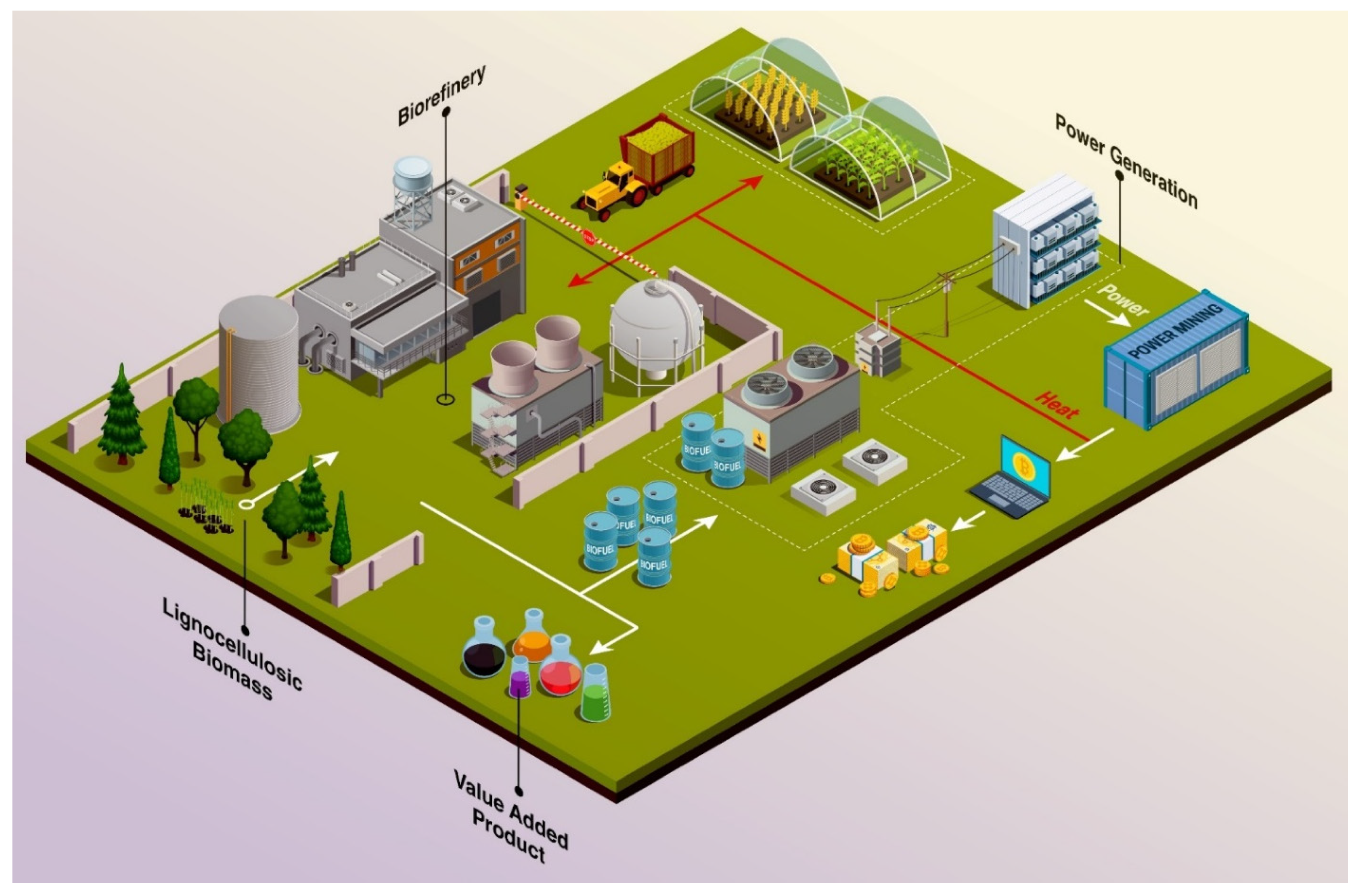
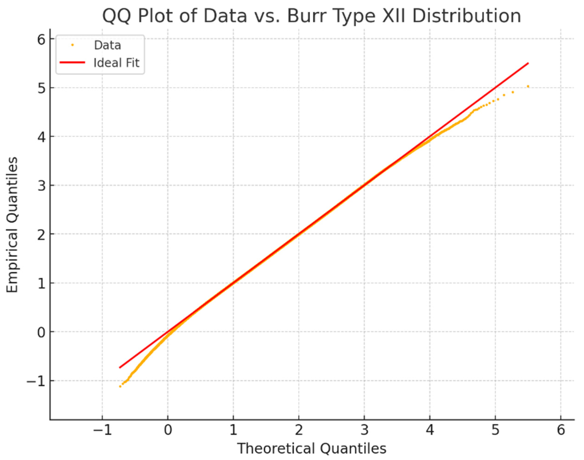
4. Results and Discussion

A set of sensitivity analyses and Monte Carlo simulations was conducted to estimate the minimum mining costs PP and profitability criteria PC. The aim was to forecast the future performance of an IB engaged in Bitcoin mining using the model equations, assumptions, and input distributions. This approach yielded a probabilistic range of outcomes rather than a single deterministic result, providing insight into variability and risk.
First, the spatial heatmaps in Figure 2 illustrate the sensitivity of PP to changes in RTOT, EOP, and ECAP, as defined by Equation (7). The baseline PP was calculated using the mean values of the parameters in Table 1. Thereafter, each of the factors RTOT, EOP, and ECAP was varied by ±50%, showcasing how PP responds to simultaneous changes in pairs of factors relative to the baseline PP. In the first heatmap, PP is shown as a function of RTOT and EOP (with ECAP held constant). The second shows PP as a function of RTOT and ECAP (with EOP held constant), and the third shows PP as a function of EOP and ECAP (with RTOT held constant). It is important to note the large variability introduced by empirically fitted variables, such as HN, HM, εM, and PBTC, which exacerbates the extremities in the PP estimate.
Second, a single-factor sensitivity analysis was performed by varying each individual input variable by ±50% and recording the resulting percentage change in the PP output, as shown in Figure 3. The most sensitive parameter was shown to be the start year, i, of the IBs mining operations, whereas the least sensitive was the initial number of ASIC units, n0. Notably, adjusting i had an extreme effect. A 50% reduction in i (starting mining operations in 2017) caused a 99.8% decrease in PP, while a 50% increase in i (starting mining operations in 2041) led to an 8616.4% increase in PP. This indicates an exceptionally high sensitivity to the timing of when Bitcoin mining commences, as well as decreasing RTOT. The magnitude of this effect also reflects the compound appreciation in BTC mined in earlier epochs. Coins rewarded at a subsidy of 12.5 BTC/block (9 July 2016 to 11 May 2020), when BTC traded at approximately USD 5000, have since appreciated twenty-fold. If an operator retains (rather than immediately sells) part of the early-epoch production, the realised present-value revenue can offset later-period inefficiencies. The IB’s total operational time, T, was also highly influential, with a 50% decrease in T reducing PP by 65.6% and a 50% increase in T raising PP by 114%. Several variables, such as CELE, PM, δM, ξM, ρINS, ρINF, θINS, θINF, σIB, σMT, and n0, showed symmetrical impacts in both ±50% scenarios, indicating a linear relationship with the changes. Meanwhile, variables such as μt, r, ω, gM, dM, gFEE, T, i, and α exhibited asymmetrical responses, suggesting non-linear effects on PP. Finally, it should be noted that empirically derived variables, such as HN, HM, εM, and PBTC, were not directly varied in this one-factor sensitivity test. However, due to their power-law dependence on t and, therefore, i, these empirically derived variables are likely a significant source of the overall sensitivity observed in PP.
Monte Carlo simulations were conducted to determine the profitability criteria PC as given in Equation (10). For the MC analysis, all model inputs were sampled from the probability distributions given in Table 1, including the residuals from the empirical power-law fits for HN, HM, εM, and PBTC. Operational time T was taken to be a uniform distribution in order to examine its effect on the PC of IBs integrating BTC mining. First, PC was simulated for each operational year by fixing T between 1 and 30, as given in Figure 4. Thereafter, PC was simulated across the entire span of T in Table 1, as given in Figure 5.
Figure 4 displays the Monte Carlo PC simulation results for each operational year between T1 and T30. As expected, the PC for each year of operation tends to decrease non-linearly due to the non-linear changes in ϕ0 and other time-sensitive parameters. Additionally, since upgrades to IB Bitcoin mining operations are simulated to occur every 4 years (i.e., years 1, 5, 9, 13, 17, 21, 25, and 29) the costs in those years are higher than others, thereby leading to noticeably lower PC values in those years, as shown by the orange bars. It should be noted that the distribution given to variable i (shifted geometric distribution with p = 0.3333 for x ≥ 16) signifies that IB Bitcoin mining operations are set to commence as early as possible, beginning in the year 2025, corresponding to year t = i = 16 and onwards.
Figure 5 displays the distribution of PC outcomes across a broader range of scenarios and operational periods. Here, T was allowed to span the entire discrete uniform distribution range allotted. Due to the extremely heavy-tailed nature of the output distribution, a log10 transformation was conducted to enhance the interpretability of the data and better visualise the Monte Carlo simulation results. While in Equation (10), profitability is measured with a PC < 1, a log10 transformation of profitability is defined as PC < 0. The Monte Carlo results underscore that profitable outcomes are statistically scarce under the given assumptions, highlighting the challenging economics of integrating Bitcoin mining into IBs. Finally, the Q-Q highlights the plausibility of the PC simulated outcomes against the fitted Burr Type XII distribution.
The model equations used for estimating the minimum profitable mining price and profitability criterion were developed and further expanded based on [47]. PP is an IB-specific threshold price, expressed in USD/BTC, at which mining operations become profitable. Essentially, PP allows for a ceteris paribus benchmark to compare between various designs, scenarios, and assumptions. A lower PP improves capital allocation efficiency by decreasing PC, so financial analysts must determine IB profitability under varying scenarios. Notably, both PP and PC are time-dependent metrics. Therefore, deterministic predictability becomes more erroneous as time begins to be considered, and a more probabilistic method is needed [48]. Likewise, as with any capital budgeting or investment appraisal, the quality of the outcome depends heavily on the input data and assumptions used.
In profitable scenarios, IBs can leverage the additional revenue from Bitcoin mining to reduce internal costs, fund expansions, or lower the prices of their VAPs for consumers. Conversely, if mining is unprofitable, an IB would be better served by diverting its biofuel output resources to alternative revenue generation methods instead of mining.
Under profitable scenarios, IBs can leverage this additional revenue stream or profit from Bitcoin mining to support internal cost reductions, business expansions, or lower VAP pricing for consumers. However, in nonprofitable situations, IBs may be better off exploring alternative uses for their produced biofuels or reallocating funds that would otherwise have been spent on Bitcoin mining. Overall, the simulations suggest far more unprofitable outcomes than profitable ones for the IB mining venture. However, these results are highly contingent on the underlying assumptions, the probabilistic distributions chosen, and the empirical models employed.

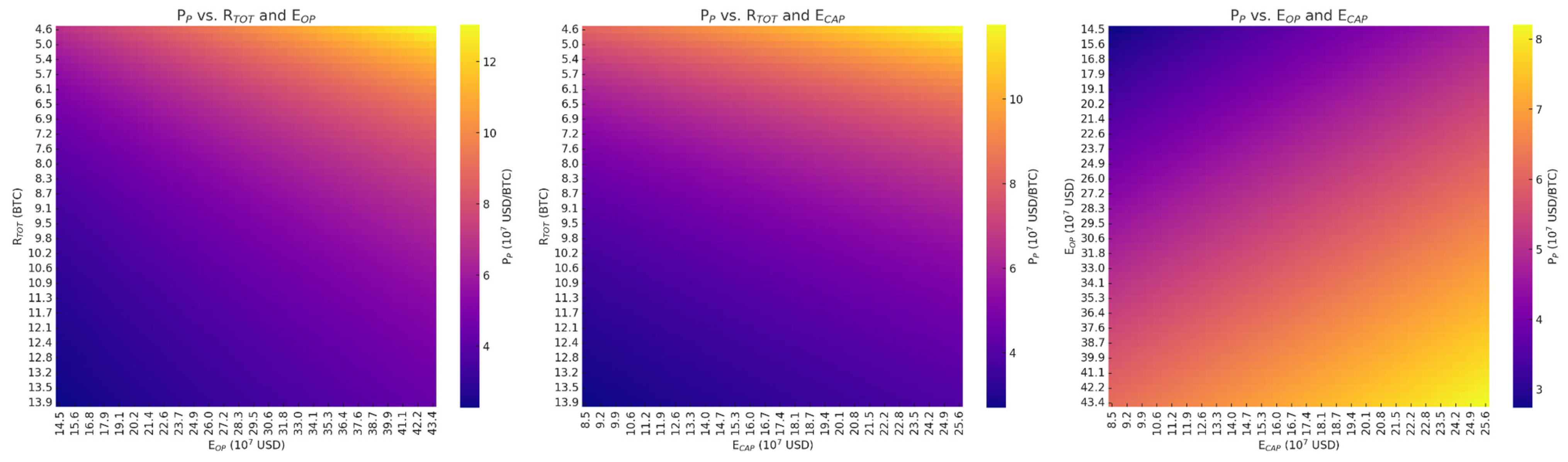
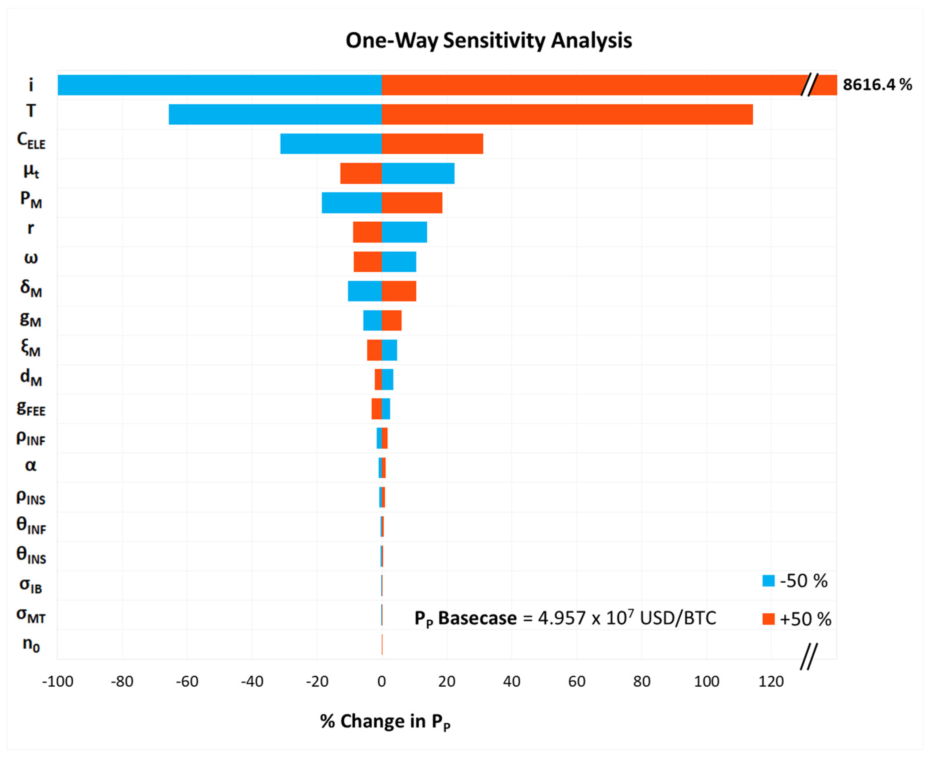
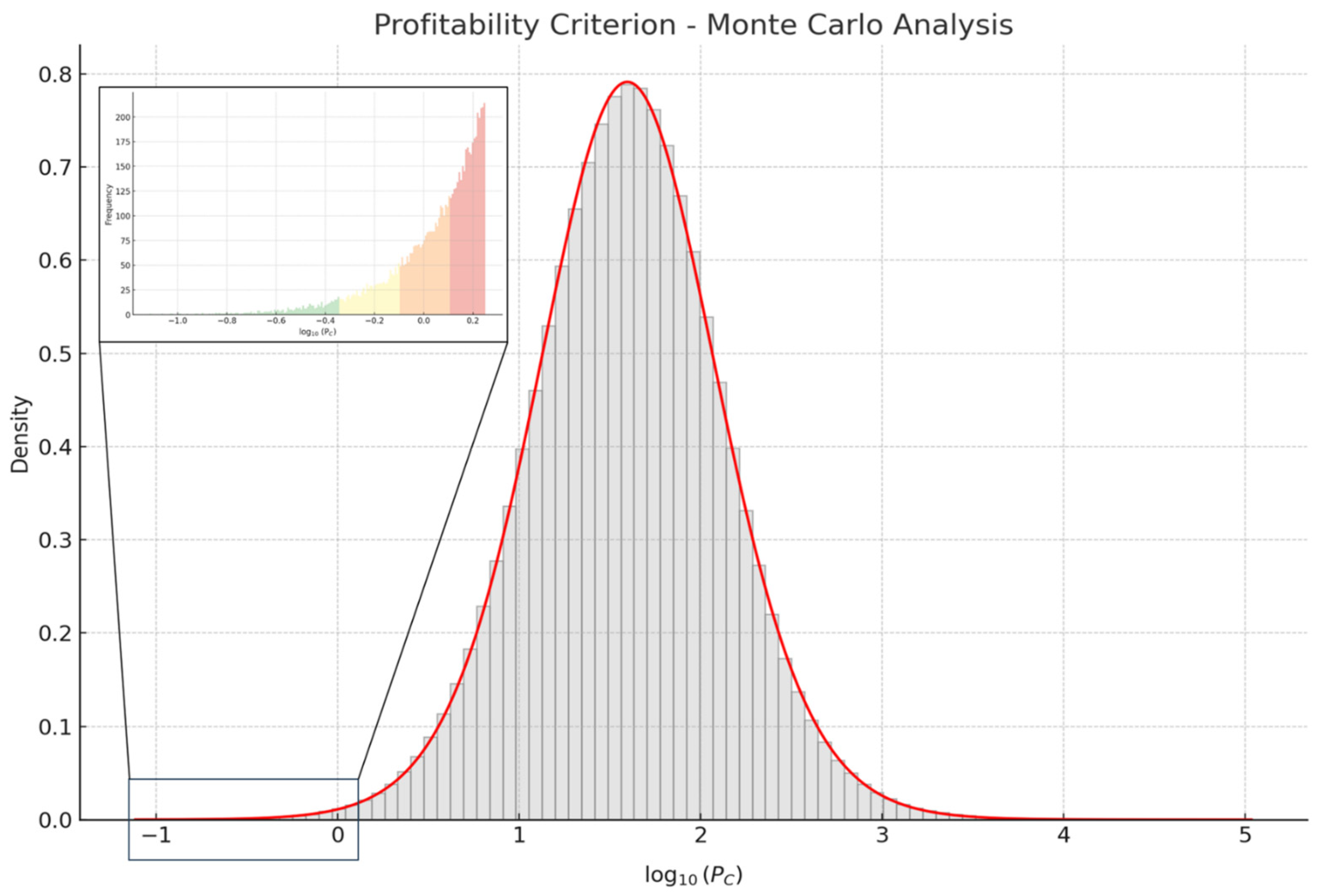
Sensitivity Analysis and Monte Carlo Simulations

In Figure 2, the PP vs. RTOT/EOP and the PP vs. RTOT/ECAP heatmaps show similar patterns, reflecting synchronous influences of these factors on PP. Logically, lower expenditures, i.e., lower ECAP and EOP, contribute to reduced PP. Increasing RTOT also aids in decreasing PP; however, this effect is inherently limited by the halving of ϕ every 210,000 blocks. Overall, PP is slightly more sensitive to changes in EOP than to ECAP, suggesting that month-to-month expenses are more critical to control. This is reinforced by the sensitivity ranking of CELE being the third most sensitive variable to control. Nevertheless, efficient capital allocation and preservation remain important for long-term sustainability. In practice, to be and stay profitable, an IB needs to maximise RTOT by utilising low-cost electricity and the most efficient ASICs while controlling and minimising EOP and ECAP by enhancing energy and cost efficiencies. As ϕ is halved every 210,000 blocks, simply running longer or adding capacity cannot overcome the programmed decline in rewards, unless PBTC reacts to this change immediately without a time lag. This reinforces that for an IB, cost efficiency, rather than scale, is the primary lever for profitability in order to mitigate against periods with low PBTC (compared to the global aggregate PP).
Figure 3 shows that PP is most sensitive to the dimension of time, specifically, the start year i. This finding aligns with prior arguments that production costs tend to rise, and PBTC,t reaches a long-run equilibrium over time [47,49]. The sensitivity analysis reveals significant variability in the impact of parameter input changes on PP output. For example, variables i, T, CELE, μt, r, and PM are highly sensitive, whereas variables such as ρINS, ρINF, θINS, θINF, σIB, σMT, α, and n0 show lower sensitivity. An IB can improve operational efficiency by focusing on the most impactful variables that it can control, while de-emphasising less critical factors for better optimisation. In particular, key controllable factors include i, T, CELE, PM and, thereby, CM, r, and ξM. By choosing a lower start year i, IB mining operations can commence earlier, which is highly important for both increasing RTOT and reducing CTOT. Also, by shortening the operational time T, IB Bitcoin miners can avoid long-term costs where RTOT has decreased. For an industrial stakeholder, the decision to integrate mining, if at all, is crucial, as delays will likely erode economic advantages. Reducing CELE directly improves the miners’ profitability further, reiterating the emphasis on the importance of lower EOP as opposed to ECAP. Additionally, if an IB acquires efficient ASIC hardware when prices are low (i.e., low PM, low CM), and then later resells it whenever PM temporarily rises, it can potentially recover most, if not all, of its previous CM costs. However, this approach carries inventory management risk and timing uncertainty. While IBs do not have complete control over the discount rate, r, it is also an important factor to consider. Borrowing at a lower cost of debt and optimising the debt-to-equity ratios allows them strategic flexibility in lowering their cost of capital. Although ξM is not amongst the highest sensitive factors, controlling it by taking advantage of ASIC bulk discounts can reduce ECAP, especially over longer periods of operation T. Greater importance should be placed on the expansion of operations (ρINS and ρINF) rather than on the initial setup (θINS and θINF), as this has a larger impact on decreasing PP. Finally, the least sensitive variable was found to be n0 since it increases RTOT but also increases ECAP and EOP in a proportional amount.
Figure 4 shows that the average probability of profitability evolves for each year of operation between T1 and T30, given the stochastic variations in key inputs. The clear downward trend indicates that cost recovery via mining becomes increasingly difficult over time due to changes in network parameters and declining mining efficiency. Early in the project, the likelihood of being profitable in a given year is modest but non-insignificant. The average probability of profitability in the first epoch (T1 to T4) is 4.52 ± 0.03%. This drastically decreases by over 95% to 0.20 ± 0.01% in the seventh epoch (T25 to T28). This already indicates that even at the outset, when ϕ is highest and new hardware is most effective, the odds are heavily stacked against IB mining profitability. Because capital costs are mostly incurred upfront, the single most profitable year is T2, where the probability of PC < 1 is 7.69 ± 0.02%. The probability of profitability decreases asymptotically, but never reaches zero, to ≈0.2% from T17 onwards. These results imply that the best strategy is to shorten the Bitcoin mining operational time whilst maximising RTOT within that mining period.
The non-linear, asymptotic decline in marginal profitability over time reflects Bitcoin’s economic design as a monetary medium with a capped supply and increasing production cost. The rarity of profitable outcomes (less than 1%) is driven by several interacting factors. First, HN,t increases over time, intensifying competition and reducing the share of mining rewards available to any single participant. Second, PBTC,t, while historically trending upward, remains volatile and unpredictable, exposing mining operations to substantial revenue risk. Third, the model’s assumption of fixed 4-year ASIC upgrade cycles introduces inflexibility compared to real-world operations, where miners may opportunistically upgrade hardware to respond to changing conditions. However, it is important to note that in today’s actual mining environment, numerous mining operations remain profitable. Model predictions for PP appear high (≈4.957 × 10⁷ USD/BTC) compared to PBTC today of approximately 100,000 USD. Therefore, the modelled scarcity of profitability reflects the inherent competitiveness and uncertainty in the mining industry rather than an intrinsic flaw in Bitcoin mining itself. Mining remains a highly dynamic and opportunistic sector, where only the most cost-efficient and agile participants consistently achieve sustainable profitability.
In a maximal scenario, the BTC value tends to converge toward the ratio between its monetary utility and the cost of energy required for its production [26]. This suggests that Bitcoin’s valuation is shaped not only by market demand but also by fundamental energetic constraints, implying a long-term stabilisation of value around energy costs. Such dynamics position Bitcoin as a digital commodity whose value is intrinsically linked to physical resource scarcity. This underpins BTC’s value proposition as a long-term store of value [41], from which an IB venture can benefit in supporting internal cost reductions, business expansions, or lower VAP pricing for consumers. For an IB, any BTC mined in earlier years could appreciate in value, potentially offsetting the fact that direct mining profits become scarce in later years. This dynamic might support strategic decisions, such as mining early and holding BTC as an asset, since the probability of profiting from operations in later years is low, but the early-mined BTC could gain value externally. Moreover, it may be prudent for IBs to evaluate whether purchasing BTC directly, rather than producing it, offers a more viable and cost-effective strategy given their specific operational context.
Overall, the Monte Carlo simulation results in a very low probability of profitability for an IB under the baseline assumptions in Table 1. The probability of profitability, and, hence, the average cost recovery, is low (P(log10 PC < 0) = 0.23%). However, whoever is able to be profitable can gain a larger market share for the VAPs, as this strategy can offset internal costs, reduce business expenses, or lower consumer prices for consumers. Four scenarios are given in the expanded section of the distribution in Figure 5. First, cases in green are extremely profitable for the entire period T. An IB in this zone would more than recover costs and generate substantial surplus value from mining, potentially using those gains to subsidise its core biorefinery operations or invest in expansion. Second, cases in yellow remain profitable, albeit with lower margins. In such cases, mining can provide a helpful supplementary income to the IB, albeit with caution. Third, cases in orange are borderline, suggesting that changes in conditions can move them between profitable and unprofitable outcomes. The prevalence of orange cases depends on input assumptions and reflects the high sensitivity of certain variables. An IB in this zone would need to be ready to adapt or exit the mining project if conditions worsen. Fourth, cases in red are the overwhelming majority and represent losses from an IB Bitcoin mining endeavour. The predominance of red outcomes is concerning, as it underscores fundamental challenges in the IB Bitcoin mining business model and market conditions that can lead to otherwise avoidable losses. It also highlights that only the most cost-efficient miners are likely to survive in the long run (lower ECAP, lower EOP, higher RTOT). A statistical fit of the simulated outcomes suggests they follow a Burr Type XII (generalised log–logistic) distribution with the following fit: c = 6.99, d = 2.79, loc = −1.12, and scale = 3.26. The Q-Q plot between the actual data and the distribution fitting is given in Figure 6. The Kolmogorov–Smirnov (KS) test gave the following parameters: KS statistic = 0.0015 and p-value = 0.0197 (<0.05). Finally, the Q-Q plot shows deviation in the tails, suggesting that the probability of extreme scenarios may be misestimated. For instance, underestimating PBTC,t and overestimating HN,t simultaneously during parameter selection will skew the results towards extremely unprofitable PC outcomes that otherwise would have been profitable.
While key variables such as ϕ, ω, βt, and t are influential, IB Bitcoin miners must acknowledge the reality that such conditions are imposed on all network participants without the ability to change for any miner participant. Furthermore, it is clear that the high sensitivity observed in ASIC miner variables, such as PM, μt, ξM, and δM, proves that capital preservation and ASIC upgrades are necessary for a sustainable IB mining over long operational periods T. Strategic management of ASIC capital is fundamental in decreasing ECAP and EOP. Moreover, access to low-cost electricity CELE significantly aids in decreasing EOP, which is a prime factor in decreasing PP, further reinforcing the notion that operational efficiency is key for a profitable mining operation within an IB. The low PC findings from Monte Carlo simulations clearly demonstrate that under the right conditions, incorporating Bitcoin mining into an IB can be a profitable venture. This supports the notion of cost recovery, as evidenced by the green, yellow, and orange zones. However, a careful case-by-case assessment of the assumptions, risks, and rewards is warranted before an IB pursues this strategy. Figure 7 provides a practical decision-making flowchart to help plant operators assess the feasibility of integrating BTC mining into IBs.

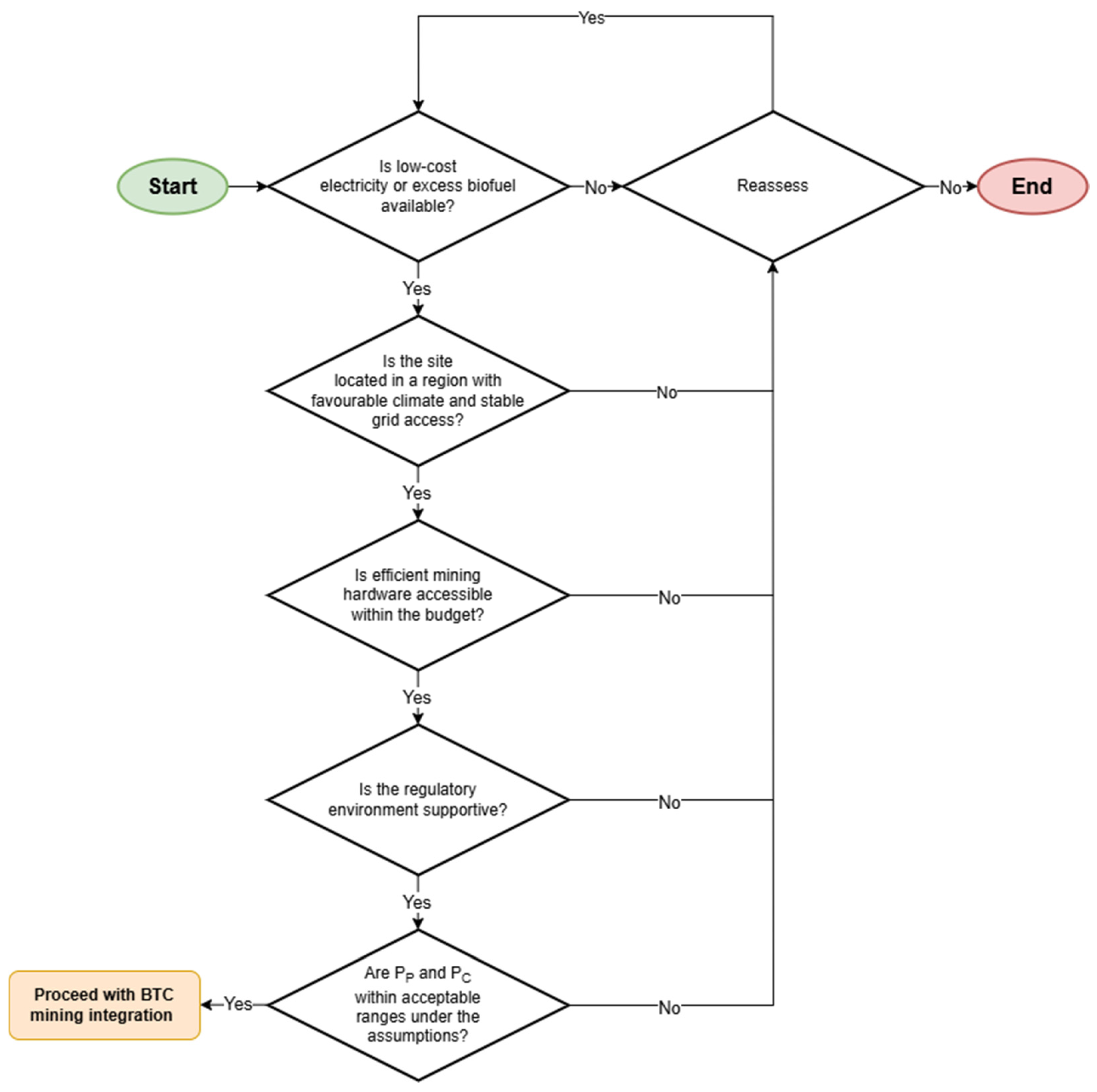
5. Model Limitations and Other Considerations

While simulations offer a structured view of profitability, they cannot fully capture the complex, dynamic reality of a long-term mining venture. Recognising these limitations is essential to avoid misinterpreting outcomes and to identify areas where further analysis is needed.
First, the model’s evaluation of profitability over the entire period T does not account for the timing and sequence of annual profits and losses. It is important to consider tail risk. In the Monte Carlo analysis, a scenario is labelled unprofitable if the cumulative outcome over T years fails to meet the profitability criterion, even if that scenario includes some highly profitable years. However, the current mode of calculations in MC analysis does not effectively distinguish these scenarios, and this tends to underestimate scenarios where early successes and prudent management could offset later failures. Second, path dependency is a critical factor, as profitability in earlier years often enables more operations and potential profitability in later years, which is not adequately reflected in the simulated outcomes. A few exceptionally good years could generate enough surplus to cover subsequent down years. The lack of path dependency in the model means the simulated outcomes may be more pessimistic than a managed real-world scenario. Third, the only revenue source generated is BTC, and the model does not account for ancillary benefits or revenues beyond the mining operation. Notably, waste heat from ASICs (for preheating, drying, or heating indoor facilities) can be monetised, which should also be considered as this adds another revenue source and decreases PC. It was shown that greenhouse tomato cultivation was more profitable when waste heat from Bitcoin mining was redirected towards it. The researchers noted that factors such as location, climate conditions, utility costs, and BTC price were important aspects supporting the process [50]. If an IB implements heat reuse, the effective energy cost of mining would be partly offset by savings or revenue elsewhere in operations.
While the average profitability over all scenarios seems low initially, the model relies on numerous assumptions about how technical and economic parameters will evolve, some of which are estimated by empirical fit and forecasted forward, thereby systemically affecting the outcomes. It is important to note the inherent uncertainty in the assumptions for any variables, most notably, the variables dependent on T, t, or i, especially over longer time horizons. The increasing variance from residual sampling results in greater output variability and wider confidence intervals as the model projects further into the future, making PC estimates more uncertain as i and T increase. For example, HRN, εM HRM, and PBTC were projected using a power-law fit extrapolated from historical data. If their actual future values deviate from this pattern, due to changes in geopolitics, technology, and macroeconomic conditions, then the PP and PC outcomes would be different. Residual sampling in the Monte Carlo simulations projects future values along smooth trajectories, which could overestimate the difficulty of mining in later years. For IBs, long-term forecasts in the Bitcoin mining context are highly speculative. Small errors in exponent parameters or growth rates compound over time, leading to large differences in later years. The Bitcoin network includes a dynamically inbuilt difficulty adjustment feature, which self-regulates every 2016 blocks. This means that extremely adverse conditions for miners would not persist indefinitely. When mining becomes less profitable and many miners cease operations, the block production rate declines. This triggers a decrease in mining difficulty, ensuring the system recalibrates to maintain a consistent average block time of ≈10 min, thereby sustaining the feasibility of mining. Such dynamics are not captured here. Power-law distributions are sensitive to changes in their tail behaviour. The model’s projections for PP and PC may understate this effect because it does not simulate miners entering or exiting in response to conditions. Instead, it presumes continuous growth in HRN. In reality, if mining profitability drops, enough miners would shut off such that the IB could benefit from this downward difficulty adjustment, thereby increasing its share of ϕ. Both PP and PC are time-dependent metrics, and it is more appropriate to evaluate them on a rolling basis rather than relying on fixed-point projections for T years into the future.
Higher prices incentivise more mining, thereby increasing the hashrate, while a rising hashrate increases mining difficulty and affects production cost. This interdependence complicates forward projections of PP and PC, especially when both inputs must be forecast simultaneously. Both HN and PBTC are time-dependent variables that influence each other. Daily HN and PBTC data collected between 17 July 2010 and 23 April 2024 show a correlation coefficient of 0.97 on a log–log scale. Historically, HN increases faster than PBTC due to rapid improvements in ASIC hardware efficiency and aggressive reinvestment strategies by miners aiming to maximise their share of ϕ before halving events. Over the long run, our model proves that the marginal profitability falls precipitously and that only the most efficient and cost-optimised operations survive.
The model also omits certain operational and financial strategies that an IB could employ. It is important to note that BTC mined in year t do not necessarily have to be sold at the spot price in year t+1; however, the analysis does not incorporate this kind of inventory/asset management. In the real world, IB management has the option to hold mined BTC as an asset rather than sell immediately. Likewise, the model assumes mining continues in a steady fashion without considering that an IB could pause or scale back operations during particularly unprofitable periods and potentially resume when conditions improve. The model also does not reflect the nature of some specific situations. For example, the treatment of ASIC costs, CM, is vastly simplified. Since CM fluctuate with PM, an IB can engage in a financial cycle of purchasing, deploying, reselling, and replacing ASICs. While PM generally declines, certain periods can see a surge of ≈400%, as seen between May 2020 and May 2021. Under favourable market conditions, such as high PM, high stable PBTC, or low stable HN, this process can be executed in such a manner that the resale value of ASICs does not deviate far from their initial purchase price, all while accounting for their depreciation. Moreover, the model’s static 4-year upgrade cycle could overstate costs since dynamic ASIC management is not included. This significantly lowers ECAP as PM and μt are the most important variables after i, T, and CELE.
Finally, even though the majority of the simulations result in loss, it is imperative to note that the sale value of VAPs produced by an IB can be brought down if one operates in the green, yellow, and orange zones, thereby proving that it is possible to utilise Bitcoin mining in IBs to make them more competitive. However, it also brings forth risk. Predictability is relatively poor and a significant challenge. The variables PM, HRN, εM HRM, and PBTC are influenced by time t, and because of this direct dependency, they significantly affect production prices and the number of profitable scenarios. Therefore, any incorrect assumptions introduced in the distribution of residuals for PM, HRN, εM HRM, and PBTC will exacerbate variability in the output, which is itself dependent on time. At the proposed production prices given here, it may be more suitable for an IB to buy BTC (using equity or debt), rather than mine it, or sweep excess cash flows into BTC and leave mining to those with the lowest costs. Nonetheless, even under the assumed conditions, PC < 1 is still achievable, albeit less so.
While the model helps create a structured approach to predict outcomes, it inevitably falls short of encapsulating the multifaceted and stochastic nature of reality. For example, unexpected technological breakthroughs, regulatory changes, or market disruptions can lead to outcomes significantly divergent from model predictions. Real-world systems often exhibit non-linear behaviours and interdependencies that are difficult to predict or quantify, such as sudden changes in miner participation due to geopolitical events or dramatic shifts in energy costs.

6. Environmental Concerns, Regulations, Risks, Opportunities, and Other Issues

Regions such as northern Norway and Sweden, Iceland, northern Canada, the USA, Paraguay, Chile, Kenya, and Zambia combine cheap renewable or stranded power, ample lignocellulosic feedstock, and naturally cool climates, making them prime sites for IBs that also mine BTC.
In terms of economic considerations, several external factors affecting broader market opportunities must be considered when evaluating IB mining operations. Bitcoin mining has already been successfully deployed as a balancing method for electrical grids by utilising excess energy production [34]. Moreover, mining is increasingly used to mitigate emissions by converting waste CH4 into energy, yielding positive environmental and economic benefits [20]. The present analysis proposes that excess energy in an IB can similarly be diverted into Bitcoin mining to generate profit to aid in financing other production operations and/or to offset the price of VAPs for consumers. IB Bitcoin miners can leverage biofuels as a renewable energy source, thereby advancing sustainability and implementing carbon reduction measures. This allows for the bridging between research, product and platform development, and market growth [19]. Using Bitcoin mining as a hedge for renewable energy investment has been demonstrated [36]. A recent study showed that using renewable energy for Bitcoin mining significantly decreases freshwater and marine eutrophication by up to 97.1%. Incentivising green hydrogen power for Bitcoin mining can enable carbon capture of at least 7.4 tCO2-eq per BTC, with potential increases up to 22.6 tCO2-eq in favourable states like Idaho (USA), depending on the local energy mix and electricity prices, potentially leading to carbon-neutral outcomes depending on actual mining emissions [30]. The same study showed that returns from Bitcoin mining produced a positive feedback loop of increased reinvestments and capacity expansion up to 25.5% and 73.2% for solar and wind power infrastructure, respectively [30]. Implementing profitable carbon capture and utilisation strategies to help neutralise emissions from BTC mining has also been discussed [51].
On the other hand, there are various risks and concerns one typically associates with BTC and Bitcoin mining. First is the heightened volatility in PBTC, whereby profitability in mining is heavily determined by the spot price, which is notorious for unpredictably moving. This volatility is attributed to the relatively young age and globally low market penetration that Bitcoin currently exhibits. However, as BTC’s market capitalisation and liquidity increase, the price swings moderate. Therefore, investments in Bitcoin mining must be accompanied by a longer-term perspective of this growing market, with buffers set in place to mitigate against short-term volatility. The second major concern is related to the consumption of energy. The decentralised PoW mining process inherently requires a large energy expenditure to secure the network, and this high energy cost is what discourages attacks and keeps the network secure. The dispersed nature of mining operations makes it challenging to account for the mix of energy sources being used at a global scale. As of 2024, Bitcoin mining uses between 80 and 240 TWh of electricity annually [52]. In comparison, domestic refrigeration, commercial banking, and video gaming use 630, 239, and 105 TWh per year, respectively [19,53]. Moreover, due to ASIC hardware efficiency gains, mining accounts for only about 0.1% of global energy consumption, with estimates that 39 to 73% of the energy comes from renewable sources [19,52,53,54]. This trend is expected to continue, with renewables and stranded energy sources making up a growing share of the mining power mix. Finally, mining is estimated to contribute only 0.06% of annual global CO2 emissions, with various studies reporting a significantly wide range of figures from 0.2 to 95.4 MtCO2 [53]. Increasing the use of renewable energy in mining, as well as implementing carbon credits or carbon taxes, have been suggested as ways to further reduce and offset mining-related emissions [35,55]. KPMG reports that Bitcoin mining incentivises the rapid deployment of renewables, enables financial inclusion, and increases security and transparency, thereby supporting the ESG framework [27,32]. Finally, the notion that Bitcoin is predominantly used for illicit activities has been refuted [19,56].
Regulatory policies will significantly impact the viability of integrating Bitcoin mining into IBs. Restrictive measures, such as on/off ramp closures, mining bans, and regressive tax policies, will likely drive the industry and its innovation to more welcoming jurisdictions. It is important to note that if PC rises above 1, miners will cease operations. Due to the network’s decentralised nature, any policies that artificially raise local costs and push PC higher will incentivise miners to relocate elsewhere (geographical arbitrage) where PC is lower. On the other hand, establishing proper monitoring and inspection regimes can improve the oversight of mining activities without unduly hampering them. Therefore, a forward-thinking, coordinated, and non-punitive regulatory framework is needed to foster an innovative environment for incorporating Bitcoin mining into IBs and other renewable energy investments [30,57]. Bitcoin mining legality varies globally. It is legal in many countries, including the US, Canada, and most of Europe. However, some nations like China have banned it [58]. Moreover, while the State of New York issued a bill banning BTC mining (2021-S6486D), other states like Texas, Wyoming, and Kentucky have introduced supportive measures, encouraging BTC mining. Additionally, future developments, such as carbon-pricing mechanisms or import duties on ASIC hardware, could materially affect operational or capital costs. In the model structure, these regulatory interventions would primarily manifest as increases in electricity costs (raising EOP) or hardware investment costs (raising ECAP). Investors should, therefore, include a jurisdictional risk screen alongside the technoeconomic criteria captured by PC. Integrating policy-shock scenarios into future extensions of the model would further enhance its robustness to regulatory uncertainty.

7. Conclusions

The introduction of Bitcoin mining into integrated lignocellulosic biorefineries represents a novel approach to enhance operational efficiency and profitability. By channelling surplus energy into Bitcoin mining, an IB can capitalise on an external revenue stream for cost recovery. Biorefineries typically rely on optimising internal production processes to increase profitability, and integrating Bitcoin mining allows them to reach external markets and resources to support economic viability. If an IB can increase its profitability through this integration, it may offset some production costs and avoid passing those costs on to consumers, potentially allowing for lower and more competitive VAP prices (e.g., ethanol, lactic acid, vanillin, levulinic acid, furfural, etc.). To that end, a probabilistic model was developed to analyse the profitability of integrating Bitcoin mining into IB operations. The results suggest that under favourable circumstances, biorefining and Bitcoin mining can form a symbiotic relationship that allows IBs to operate more competitively. However, Bitcoin mining is an exceptionally competitive industry, always seeking lower costs (low EOP and ECAP) for higher revenues (RTOT), which is itself decreasing. The findings indicate that to achieve profitability and cost recovery, an IB must manage its energy costs CELE, maximise its capital efficiency PM, μt, and δM, and secure funding at a lower cost of capital r. Equally important is starting as early as possible, by minimising the start time i and the operational duration T.
Mining is a low-margin industry. In practice, only IBs with access to low-cost electricity, typically achieved through location-specific advantages, curtailment agreements, dynamic pricing mechanisms, or grid-level incentives (such as the case of Riot Platforms and ERCOT, Texas or Marathon Digital Holdings) are likely to remain viable over the long term. Additionally, factors such as high-efficiency ASIC hardware, medium to large-scale IBs, and effective waste heat utilisation further contribute to sustained feasibility.
In the cases where Bitcoin mining is profitable, an IB can potentially recover a portion of its costs and proportionally lower its VAP prices by that amount, thereby making its products more competitive. Conversely, if the mining venture is not favourable, it could add extra costs to the IB that are not recuperated. Whilst the results show grossly unprofitable scenarios, it is crucial to differentiate between the claim that it is universally unprofitable for an IB to engage in Bitcoin mining and the more nuanced conclusion that profitability depends on specific circumstances. While many simulated events are unprofitable, the model results reflect just one possible scenario within a broader range of outcomes, which can vary based on user-selected distributions, empirical data fits, and other factors. The modular nature of the model and inputs can serve as a valuable tool for decision-makers in evaluating investment opportunities, risk management, and strategic planning. By providing insight into cost structures and profitability under varied conditions, it enables IB operators to make informed decisions aligned with their goals and prevailing market dynamics. A collaborative business model that shares both risk and reward between biorefinery operators and Bitcoin mining stakeholders may help in effectively merging the two industries.
Finally, it is important to note that the model and assessment pertain only to PoW digital assets, specifically Bitcoin. This does not extend to other digital assets as they do not achieve network consensus through difficulty-adjusted PoW.

Author Contributions

G.S.—conceptualisation, methodology, formal analysis, investigation, visualisation, project administration, writing—original draft, and writing—review and editing. G.W.—methodology, writing—original draft, and writing—review and editing. T.D.—supervision, methodology, and writing—review and editing. G.K.—supervision and writing—review and editing. All authors have read and agreed to the published version of the manuscript.

Funding

This research received no external funding.

Data Availability Statement

Data will be made available on request.

Conflicts of Interest

The authors declare no conflicts of interest.

Nomenclature

P P Minimum profitable mining price.
C T O T Total cost over mining operational time.
E C A P Capital expenditure over mining operational time.
E O P Operational expenditure over mining operational time.
R T O T Total Bitcoin revenue over mining operational time.
P C Profitability criterion.
P B T C Bitcoin spot price.
n t Number of ASICs.
n B T C Number of Bitcoin mined during year t.
g M Growth rate in number of ASICs over epoch.
d M Decay rate in number of ASICs over epoch.
P M Cost of computation per ASIC.
μ t Year-over-year decrease in the cost of computation.
σ I B IB-specific costs related to mining.
C M Total ASIC cost.
ξ M Bulk discount for large ASIC purchases.
δ M Annual percentage ASIC depreciation.
r t Discount rate.
θ I N F Cost fraction assigned to infrastructure at t = i.
θ I N S Cost fraction assigned to installation at t = i.
ρ I N F Cost fraction assigned to infrastructure at τ.
ρ I N S Cost fraction assigned to installation at τ.
σ M T Maintenance-related costs.
C E L E Cost of electricity.
H M ASIC hashrate.
ε M ASIC efficiency.
H N Total network hashrate.
ϕ 0 Bitcoin block subsidy.
ω Bitcoin fees per block.
g F E E Fee growth rate.
α Mining pool fees.
β Number of blocks generated per year.
t Current year.
i Initial year of operation.
T Total operational time.
τ Epoch (210,000 blocks ≈ 4 years).

References

  1. Ning, P.; Yang, G.; Hu, L.; Sun, J.; Shi, L.; Zhou, Y.; Wang, Z.; Yang, J. Recent advances in the valorization of plant biomass. Biotechnol. Biofuels 2021, 14, 102. [Google Scholar] [CrossRef] [PubMed]
  2. González-González, R.B.; Iqbal, H.M.N.; Bilal, M.; Parra-Saldívar, R. (Re)-thinking the bio-prospect of lignin biomass recycling to meet Sustainable Development Goals and circular economy aspects. Curr. Opin. Green Sustain. Chem. 2022, 38, 100699. [Google Scholar] [CrossRef]
  3. Dahmen, N.; Lewandowski, I.; Zibek, S.; Weidtmann, A. Integrated lignocellulosic value chains in a growing bioeconomy: Status quo and perspectives. GCB Bioenergy 2019, 11, 107–117. [Google Scholar] [CrossRef]
  4. Macias Aragonés, M.; de la Viña Nieto, G.; Nieto Fajardo, M.; Páez Rodríguez, D.; Gaffey, J.; Attard, J.; McMahon, H.; Doody, P.; Anda Ugarte, J.; Pérez-Camacho, M.N.; et al. Digital Innovation Hubs as a Tool for Boosting Biomass Valorisation in Regional Bioeconomies: Andalusian and South-East Irish Case Studies. J. Open Innov. Technol. Mark. Complex. 2020, 6, 115. [Google Scholar] [CrossRef]
  5. Bhatia, S.K.; Jagtap, S.S.; Bedekar, A.A.; Bhatia, R.K.; Patel, A.K.; Pant, D.; Rajesh Banu, J.; Rao, C.V.; Kim, Y.-G.; Yang, Y.-H. Recent developments in pretreatment technologies on lignocellulosic biomass: Effect of key parameters, technological improvements, and challenges. Bioresour. Technol. 2020, 300, 122724. [Google Scholar] [CrossRef]
  6. Patel, A.; Shah, A.R. Integrated lignocellulosic biorefinery: Gateway for production of second generation ethanol and value added products. J. Bioresour. Bioprod. 2021, 6, 108–128. [Google Scholar] [CrossRef]
  7. Clauser, N.M.; Felissia, F.E.; Area, M.C.; Vallejos, M.E. A framework for the design and analysis of integrated multi-product biorefineries from agricultural and forestry wastes. Renew. Sustain. Energy Rev. 2021, 139, 110687. [Google Scholar] [CrossRef]
  8. Vu, H.P.; Nguyen, L.N.; Vu, M.T.; Johir, M.A.H.; McLaughlan, R.; Nghiem, L.D. A comprehensive review on the framework to valorise lignocellulosic biomass as biorefinery feedstocks. Sci. Total Environ. 2020, 743, 140630. [Google Scholar] [CrossRef]
  9. Ioannidou, S.M.; Galanopoulos, C.; Ladakis, D.; Koutinas, A. Chapter 21—Techno-economic evaluation and life-cycle assessment of integrated biorefineries within a circular bioeconomy concept. In Biomass, Biofuels, Biochemicals; Varjani, S., Pandey, A., Bhaskar, T., Mohan, S.V., Tsang, D.C.W., Eds.; Elsevier: Amsterdam, The Netherlands, 2022; pp. 541–556. [Google Scholar] [CrossRef]
  10. Sharma, V.; Tsai, M.-L.; Nargotra, P.; Chen, C.-W.; Sun, P.-P.; Singhania, R.R.; Patel, A.K.; Dong, C.-D. Journey of lignin from a roadblock to bridge for lignocellulose biorefineries: A comprehensive review. Sci. Total Environ. 2023, 861, 160560. [Google Scholar] [CrossRef]
  11. Yuan, Z.; Bals, B.D.; Hegg, E.L.; Hodge, D.B. Technoeconomic evaluation of recent process improvements in production of sugar and high-value lignin co-products via two-stage Cu-catalyzed alkaline-oxidative pretreatment. Biotechnol. Biofuels Bioprod. 2022, 15, 45. [Google Scholar] [CrossRef]
  12. Martinez-Hernandez, E.; Cui, X.; Scown, C.D.; Amezcua-Allieri, M.A.; Aburto, J.; Simmons, B.A. Techno-economic and greenhouse gas analyses of lignin valorization to eugenol and phenolic products in integrated ethanol biorefineries. Biofuels Bioprod. Biorefin. 2019, 13, 978–993. [Google Scholar] [CrossRef]
  13. Halder, P.; Shah, K. Techno-economic analysis of ionic liquid pre-treatment integrated pyrolysis of biomass for co-production of furfural and levoglucosenone. Bioresour. Technol. 2023, 371, 128587. [Google Scholar] [CrossRef] [PubMed]
  14. Seufitelli, G.V.S.; El-Husseini, H.; Pascoli, D.U.; Bura, R.; Gustafson, R. Techno-economic analysis of an integrated biorefinery to convert poplar into jet fuel, xylitol, and formic acid. Biotechnol. Biofuels Bioprod. 2022, 15, 143. [Google Scholar] [CrossRef]
  15. Morakile, T.; Mandegari, M.; Farzad, S.; Görgens, J.F. Comparative techno-economic assessment of sugarcane biorefineries producing glutamic acid, levulinic acid and xylitol from sugarcane. Ind. Crops Prod. 2022, 184, 115053. [Google Scholar] [CrossRef]
  16. Nakamoto, S. Bitcoin: A Peer-to-Peer Electronic Cash System; 2008; p. 9. Available online: https://bitcoin.org/bitcoin.pdf (accessed on 5 March 2023).
  17. Wang, G.; Hausken, K. Unravelling the global landscape of Bitcoin research: Insights from bibliometric analysis. Technol. Anal. Strateg. Manag. 2024, 1–18. [Google Scholar] [CrossRef]
  18. Sánchez Bayón, A.; García Ramos, M.Á. A win-win case of CSR 3.0 for wellbeing economics: Digital currencies as a tool to improve the personnel income, the environmental respect & the general wellness. REVESCO. Rev. Estud. Coop. 2021, 138, e75564. [Google Scholar] [CrossRef]
  19. Velický, M. Renewable Energy Transition Facilitated by Bitcoin. ACS Sustain. Chem. Eng. 2023, 11, 3160–3169. [Google Scholar] [CrossRef]
  20. Rudd, M.A.; Jones, M.; Sechrest, D.; Batten, D.; Porter, D. An integrated landfill gas-to-energy and Bitcoin mining framework. J. Clean. Prod. 2024, 472, 143516. [Google Scholar] [CrossRef]
  21. Ehyaei, M.A.; Esmaeilion, F.; Shamoushaki, M.; Afshari, H.; Das, B. The feasibility study of the production of Bitcoin with geothermal energy: Case study. Energy Sci. Eng. 2024, 12, 755–770. [Google Scholar] [CrossRef]
  22. Moreno, D.; Antoli, M.; Quintana, D. Benefits of investing in cryptocurrencies when liquidity is a factor. Res. Int. Bus. Financ. 2022, 63, 101751. [Google Scholar] [CrossRef]
  23. Velvizhi, G.; Balakumar, K.; Shetti, N.P.; Ahmad, E.; Kishore Pant, K.; Aminabhavi, T.M. Integrated biorefinery processes for conversion of lignocellulosic biomass to value added materials: Paving a path towards circular economy. Bioresour. Technol. 2022, 343, 126151. [Google Scholar] [CrossRef] [PubMed]
  24. Li, J.; Li, Y. Micro gas turbine: Developments, applications, and key technologies on components. Propuls. Power Res. 2023, 12, 1–43. [Google Scholar] [CrossRef]
  25. Semaan, G.; Wang, G.; Vo, Q.S.; Kumar, G. The Potential Relationship between Biomass, Biorefineries, and Bitcoin. Sustainability 2024, 16, 7919. [Google Scholar] [CrossRef]
  26. Semret, N. Dynamics of Bitcoin mining. arXiv 2022, arXiv:2201.06072. [Google Scholar] [CrossRef]
  27. Rudd, M.A.; Bratcher, L.; Collins, S.; Branscum, D.; Carson, M.; Connell, S.; David, E.; Gronowska, M.; Hess, S.; Mitchell, A.; et al. Bitcoin and Its Energy, Environmental, and Social Impacts: An Assessment of Key Research Needs in the Mining Sector. Challenges 2023, 14, 47. [Google Scholar] [CrossRef]
  28. Rudd, M.A. Bitcoin Is Full of Surprises. Challenges 2023, 14, 27. [Google Scholar] [CrossRef]
  29. Lal, A.; Niaz, H.; Liu, J.J.; You, F. Can bitcoin mining empower energy transition and fuel sustainable development goals in the US? J. Clean. Prod. 2024, 439, 140799. [Google Scholar] [CrossRef]
  30. Lal, A.; You, F. Climate sustainability through a dynamic duo: Green hydrogen and crypto driving energy transition and decarbonization. Proc. Natl. Acad. Sci. USA 2024, 121, e2313911121. [Google Scholar] [CrossRef]
  31. Lal, A.; Zhu, J.; You, F. From Mining to Mitigation: How Bitcoin Can Support Renewable Energy Development and Climate Action. ACS Sustain. Chem. Eng. 2023, 11, 16330–16340. [Google Scholar] [CrossRef]
  32. KPMG. Bitcoin’s Role in the ESG Imperative: An Overview of the Opportunities and Creative Approaches That Deliver Value and Drive Trust with Key Stakeholders; KPMG LLP.: London, UK, 2023; Available online: https://kpmg.com/kpmg-us/content/dam/kpmg/pdf/2023/bitcoins-role-esg-imperative.pdf (accessed on 29 May 2024).
  33. Malfuzi, A.; Mehr, A.S.; Rosen, M.A.; Alharthi, M.; Kurilova, A.A. Economic viability of bitcoin mining using a renewable-based SOFC power system to supply the electrical power demand. Energy 2020, 203, 117843. [Google Scholar] [CrossRef]
  34. Niaz, H.; Liu, J.J.; You, F. Can Texas mitigate wind and solar curtailments by leveraging bitcoin mining? J. Clean. Prod. 2022, 364, 132700. [Google Scholar] [CrossRef]
  35. Ghaebi Panah, P.; Bornapour, M.; Cui, X.; Guerrero, J.M. Investment opportunities: Hydrogen production or BTC mining? Int. J. Hydrogen Energy 2022, 47, 5733–5744. [Google Scholar] [CrossRef]
  36. Bastian-Pinto, C.L.; Araujo, F.V.d.S.; Brandão, L.E.; Gomes, L.L. Hedging renewable energy investments with Bitcoin mining. Renew. Sustain. Energy Rev. 2021, 138, 110520. [Google Scholar] [CrossRef]
  37. Snytnikov, P.; Potemkin, D. Flare gas monetization and greener hydrogen production via combination with cryptocurrency mining and carbon dioxide capture. iScience 2022, 25, 103769. [Google Scholar] [CrossRef]
  38. Treiblmaier, H. A comprehensive research framework for Bitcoin’s energy use: Fundamentals, economic rationale, and a pinch of thermodynamics. Blockchain Res. Appl. 2023, 4, 100149. [Google Scholar] [CrossRef]
  39. Andoni, M.; Robu, V.; Flynn, D.; Abram, S.; Geach, D.; Jenkins, D.; McCallum, P.; Peacock, A. Blockchain technology in the energy sector: A systematic review of challenges and opportunities. Renew. Sustain. Energy Rev. 2019, 100, 143–174. [Google Scholar] [CrossRef]
  40. Podhorsky, A. Bursting the bitcoin bubble: Do market prices reflect fundamental bitcoin value? Int. Rev. Financ. Anal. 2024, 93, 103158. [Google Scholar] [CrossRef]
  41. Ammous, S.; D’Andrea, F.A.M.C. Hard Money and Time Preference: A Bitcoin perspective. MISES Interdiscip. J. Philos. Law Econ. 2022, 10, 1–17. [Google Scholar] [CrossRef]
  42. Borodin, A.; Mityushina, I.; Streltsova, E.; Kulikov, A.; Yakovenko, I.; Namitulina, A. Mathematical Modeling for Financial Analysis of an Enterprise: Motivating of Not Open Innovation. J. Open Innov. Technol. Mark. Complex. 2021, 7, 79. [Google Scholar] [CrossRef]
  43. Power, A.J. Bitcoin Mining Industry Report. Available online: https://education.compassmining.io/education/bitcoin-mining-industry-report/ (accessed on 2 May 2025).
  44. Santostasi, G. The Bitcoin Power Law Theory. Available online: https://giovannisantostasi.medium.com/the-bitcoin-power-law-theory-962dfaf99ee9 (accessed on 24 April 2024).
  45. Santostasi, G. The Physics of Bitcoin. Available online: https://giovannisantostasi.medium.com/btc-is-a-power-law-because-it-is-an-infinite-recursive-feedback-loop-5f54de5e501b (accessed on 24 April 2024).
  46. Luxor. Bitcoin ASIC Price Index. Luxor Technology Corp. Available online: https://data.hashrateindex.com/chart/asic-price-index (accessed on 30 April 2024).
  47. Hayes, A.S. Cryptocurrency value formation: An empirical study leading to a cost of production model for valuing bitcoin. Telemat. Inform. 2017, 34, 1308–1321. [Google Scholar] [CrossRef]
  48. Murthy, G.S. Chapter TWO—Techno-economic assessment. In Biomass, Biofuels, Biochemicals; Murthy, G.S., Gnansounou, E., Khanal, S.K., Pandey, A., Eds.; Elsevier: Amsterdam, The Netherlands, 2022; pp. 17–32. [Google Scholar] [CrossRef]
  49. Kristoufek, L. Bitcoin and its mining on the equilibrium path. Energy Econ. 2020, 85, 104588. [Google Scholar] [CrossRef]
  50. Asgari, N.; McDonald, M.T.; Pearce, J.M. Energy Modeling and Techno-Economic Feasibility Analysis of Greenhouses for Tomato Cultivation Utilizing the Waste Heat of Cryptocurrency Miners. Energies 2023, 16, 1331. [Google Scholar] [CrossRef]
  51. Niaz, H.; Shams, M.H.; Liu, J.J.; You, F. Mining bitcoins with carbon capture and renewable energy for carbon neutrality across states in the USA. Energy Environ. Sci. 2022, 15, 3551–3570. [Google Scholar] [CrossRef]
  52. CCAF. Cambridge Bitcoin Electricity Consumption Index (CBECI). Cambridge Centre for Alternative Finance (CCAF). Available online: https://ccaf.io/cbnsi/cbeci (accessed on 29 May 2024).
  53. Tomatsu, Y.; Han, W. Bitcoin and Renewable Energy Mining: A Survey. Blockchains 2023, 1, 90–110. [Google Scholar] [CrossRef]
  54. Blandin, A.; Pieters, G.; Wu, Y.; Eisermann, T.; Dek, A.; Taylor, S.; Njoki, D. 3rd Global Cryptoasset Benchmarking Study; Cambridge Centre for Alternative Finance: Cambridge, UK, 2020; Available online: https://www.jbs.cam.ac.uk/faculty-research/centres/alternative-finance/publications/3rd-global-cryptoasset-benchmarking-study/ (accessed on 29 May 2024).
  55. Miśkiewicz, R.; Matan, K.; Karnowski, J. The Role of Crypto Trading in the Economy, Renewable Energy Consumption and Ecological Degradation. Energies 2022, 15, 3805. [Google Scholar] [CrossRef]
  56. Butler, S. Criminal use of cryptocurrencies: A great new threat or is cash still king? J. Cyber Policy 2019, 4, 326–345. [Google Scholar] [CrossRef]
  57. Mikhaylov, A. Cryptocurrency Market Analysis from the Open Innovation Perspective. J. Open Innov. Technol. Mark. Complex. 2020, 6, 197. [Google Scholar] [CrossRef]
  58. Griffith, T.; Clancey-Shang, D. Cryptocurrency regulation and market quality. J. Int. Financ. Mark. Inst. Money 2023, 84, 101744. [Google Scholar] [CrossRef]
Figure 1. A schematic representation of an integrated biorefinery system integrating lignocellulosic biomass, biofuel production, VAP production, and Bitcoin mining.
Systems 13 00359 g001
Figure 2. Sensitivity analysis heatmap illustrating the relationships between the minimum profitable mining price (PP) and key economic variables, such as total revenue (RTOT), operational expenditure (EOP), and capital expenditure (ECAP).
Systems 13 00359 g002
Figure 3. One−way sensitivity analysis displaying the impact of various model factors on the minimum profitable mining price (PP). The horizontal bars show the percentage change in PP relative to a ±50% change in the model factors.
Systems 13 00359 g003
Figure 4. Probability of profitability (PC < 1) for operational time between T1 and T30. Probability of profitability is calculated using the mean values of the model parameters in Table 1.
Systems 13 00359 g004
Figure 5. Monte Carlo simulation analysis showcasing a log10(PC) histogram over the entire design space and assumed distributions in Table 1. The red line is the Burr Type XII distribution, aka. Generalised Log–Logistic Distribution. The green and yellow zones are profitable scenarios. The orange zone is both profitable and nonprofitable scenarios with the ability to change. The red zone showcases nonprofitable IB Bitcoin mining operations.
Systems 13 00359 g005
Figure 6. Quantile–quantile plot between the Monte Carlo simulation results and a distribution fitting Burr Type XII. The Burr Type XII distribution fails to fully capture the behaviour of the data, especially at the tails.
Systems 13 00359 g006
Figure 7. Decision-making flowchart for evaluating Bitcoin mining integration feasibility for biorefinery operators.
Systems 13 00359 g007
Table 1. Variable distribution assignment.
Parameter InformationStatistics
ParameterUnitsDistributionMeanStandard Deviation5th Percentile95th Percentile
TYearsDiscrete Uniform Distribution (min = 6; max = 34) a208.087.432.6
σIBUSD/ASIC/yearLog-Normal Distribution (μ = 4.771; σ = 0.339) a12543.667.6206.2
n0-Discrete Negative Binomial Distribution (n = 3; p = 0.004) a747432.12021569
r%/yearGamma Distribution (k = 3.274; θ = 0.0226) a0.0740.0410.0220.151
δM%/yearBeta Distribution (α = 13.4; β = 4.7; min = 0; max = 0.25) a0.1850.0250.140.222
θINS%Beta Distribution (α = 19.8; β = 79.2) a0.20.040.1380.269
θINF%Beta Distribution (α = 16.4; β = 49.3) a0.250.0530.1670.341
ρINS%Beta Distribution (α = 10.8; β = 205.2) a0.050.0150.0280.076
ρINF%Beta Distribution (α = 15.6; β = 139.7) a0.100.0240.0640.142
σMTUSD/ASIC/yearLog-Normal Distribution (μ = 4.272; σ = 0.301) a7523.143.7117.6
gFEE%/yearWeibull Distribution (k = 3.434; λ = 0.0834) a0.0750.0240.0350.115
α%Gamma Distribution (k = 11; θ = 0.002) a0.0220.00660.01230.0339
βBlocks/yearDiscrete Binomial Distribution (n = 525000; p = 0.1) a52,500217.452,14352,858
iYearShifted Geometric Distribution (p = 0.3333) for x ≥ 16 a, b182.4481623
CELEUSD/kWyearLog-Normal Distribution (μ = 6.594; σ = 0.389) a788.1318.6385.31385.5
gM%/yearGamma Distribution (k = 3.333; θ = 0.03) a0.10.0550.0290.204
dM%/yearGamma Distribution (k = 8.333; θ = 0.03) a0.250.0870.1270.407
ξM%Beta Distribution (α = 15.3; β = 61.2) a0.20.0450.1290.279
μt%Gamma Distribution (k = 6.245; θ = 0.0142) a0.0880.0350.0390.154
PMUSD/TH/sInverse Gaussian Distribution (μ = 44.115; λ = 40.168) c44.11546.2327.586132.531
ωBitcoin/BlockLog-Normal Distribution (σ = 1.1336; loc = 0.0157; scale = 0.2054) c0.40620.63150.04751.3412
HN,t eTH/sTriangular Distribution (c = 0.689; loc = −1.409; scale = 2.531) c0.0160.529−0.9390.807
HM,t eTH/sSkew-Normal Distribution (a = −3.392; loc = 0.205; scale = 0.266) c0.00140.1712−0.31630.238
εM,t ekW/TH/sNormal Distribution (μ = 0; σ = 0.075) c00.075−0.1230.123
PBTC,t eUSD/BitcoinExponentially Modified Gaussian Distribution (k = 4.0165; loc = −0.3529; scale = 0.0877) c−0.00050.3631−0.38840.7136
ϕ0Bitcoin/BlockDiscrete Uniform Distribution (min = 50; max = 50) d5005050
a—Distribution assumed. b—Shifted geometric distribution (p = 0.3333) for x ≥ 16 ≡ geometric distribution (p = 0.3333) + uniform distribution (min = 16; max = 16). i = 16 signifies the start of the mining operation in 2025. For example, if an IB chooses to start mining operations in 2029, then i = 20, and so on. c—Distribution fit to available data, either with Python SciPy v1.14.0 or ModelRisk by Vose. d—Constant. e—Residuals in log10 scale.
Disclaimer/Publisher’s Note: The statements, opinions and data contained in all publications are solely those of the individual author(s) and contributor(s) and not of MDPI and/or the editor(s). MDPI and/or the editor(s) disclaim responsibility for any injury to people or property resulting from any ideas, methods, instructions or products referred to in the content.

