ArchiMate-Based System of Systems Resilience Evaluation Approach ^†

Abstract

The system of systems (SoS) is essential for integrating independent systems to meet increasing service demands. However, its growing complexity leads to disruptions that are difficult to predict and mitigate, making resilience analysis a critical aspect of SoS development. Resilience reflects an SoS’s ability to absorb and adapt to disruptions, yet its quantitative assessment remains challenging due to diverse stakeholders. To address this, we propose a model-based approach leveraging ArchiMate for SoS visualization and quantitative modeling, combined with a resilience indicator derived from model simulations. This indicator identifies critical constituent systems (CSs) and informs resilient design strategies. Using Mobility as a Service (MaaS) as a case study, we demonstrate how the proposed method can be implemented in a specific SoS.

1. Introduction

SoS refers to a set of systems or system elements that interact to provide a unique capability that none of the CSs can accomplish on their own [1]. This concept is increasingly appearing in critical infrastructure and services, such as cross-regional electrical grid systems, globalized logistics systems, and multi-modal transportation networks. Its characteristics include the operational independence of individual systems, the managerial independence of the systems, geographical distribution, emergent behavior, and evolutionary development [2]. Conventional safety engineering methods primarily focus on predicting and preventing potential risks [3]. However, in SoS, anticipating all potential disruptions and identifying structural risks is challenging due to its inherent complexity and emergence. Moreover, a minor error can be magnified and result in significant consequences due to interdependence. A notable example is the 2021 Suez Canal blockage, where a single vessel obstruction disrupted the global logistics SoS. This disruption led to worldwide supply chain breakdowns, halted production across multiple industries, and resulted in an estimated economic loss of USD 15 to 17 billion [4]. Therefore, evaluating resilience in the SoS design is crucial in ensuring its dependability [5].

Resilience refers to the ability to absorb and adapt in a changing environment [6,7]. “Absorb” reflects the remaining performance of the system after a disruption, while “adapt” describes the response and recovery process from this lowest level to a stable performance level. It has been widely studied in various domains, including organizational, social, economic, and engineering domains [8]. Resilience is an emergent structural property, meaning that its evaluation must consider not only the system’s ability to respond to specific disruptions but also the overall structure of the SoS [9]. Therefore, model-based approaches are well suited for identifying structural risks and assessing resilience. One significant barrier to SoS resilience evaluation is the involvement of independent and diverse stakeholders. Unlike traditional systems with closely coordinated stakeholders, SoS stakeholders are highly autonomous and dispersed, often operating without direct awareness of one another. This necessitates a resilience indicator that considers stakeholder interests and conflicts [10].

To address these challenges, we propose a model-based SoS resilience evaluation approach that incorporates multistakeholder perspectives to support resilience-oriented design. This approach extends workshop research [11]. The key contributions of this study are as follows:

1.

An SoS modeling and simulation approach is proposed based on ArchiMate, an enterprise architecture (EA) modeling language which facilitates a shared understanding among stakeholders. Furthermore, we introduce a quantification of model elements and relationships between them, supporting simulation-based resilience evaluation.

2.

A stakeholder-centric resilience metric is proposed. This metric takes the interests of four stakeholder categories into account: users, SoS organizers, CS providers, and society. Among these stakeholders, a cooperative game is employed to determine the consensus on resilience metric.

3.

A case study on MaaS is implemented. We apply the proposed approach to develop an SoS model for MaaS and evaluate its resilience. Through this evaluation, we identify resilience bottlenecks within the MaaS, providing insights for resilience improvement.

2. Related Works

2.1. SoS Modeling and Simulation

Early SoS research was primarily focused on addressing the definition of SoS and delineating its boundaries in relation to a single system [12,13]. In the late 20th century, some scholars began exploring the architectural aspects of SoS, attempting to employ specific terms and graphical elements to depict the constituents of SoS and provide fundamental principles for constructing overall architectures [2,14,15]. As the concept of SoS gradually crystallized, spurred by advancements in IT technology and driven by evolving demands, mature frameworks for SoS emerged. The initial efforts were observed in the military domain, where the United States Department of Defense introduced the Department of Defense Architecture Framework (DoDAF) as a foundational approach to SoS modeling. DoDAF excels in modeling mission-critical systems with detailed capability, operational, and technical views, making it ideal for a structured, defense-oriented system of systems; however, its complexity and specialization may limit its flexibility and adaptability in open, enterprise-level contexts. Subsequently, a series of SoS modeling and simulation approaches evolved from DoDAF, leading to frameworks such as the Ministry of Defence Architecture Framework (MODAF) and the Unified Architecture Framework (UAF) [16,17,18,19]. In the field of software engineering, modeling languages such as UML [20] and SysML [21,22] have also been employed for modeling SoSs that are closely tied to information technology, owing to their mature modeling languages and simulation capabilities. For cross-industry SoSs, High-Level Architecture (HLA) provides a universal standard for interaction, aiding in the establishment of heterogeneous SoS models [23]. Furthermore, certain frameworks from the EA domain, such as the Zachman Framework [24] and The Open Group Architecture Framework (TOGAF) [25], along with modeling tools like Business Process Model and Notation (BPMN) [26], have been utilized to guide the modeling of SoS from perspectives related to requirements and management. Among these, TOGAF enables holistic and flexible modeling of complex organizational systems, facilitating mutual understanding among cross-domain stakeholders by explicitly linking business objectives, operational processes, and technical architectures.

Alternative approaches originate from systems engineering. One prominent category is continuous modeling techniques, exemplified by System Dynamics (SD), which is commonly used for modeling physical SoS. For instance, Watson [27,28] utilized SD to model ecological SoS to analyze fluctuations in biological populations. Kumar [29] employed bond graphs to model autonomous vehicles and simulated the model using SD based on physical differential equations. Furthermore, Zhou [30] utilized the Functional Resonance Analysis Method (FRAM) to model healthcare-related SoSs, encompassing simulation of inherent uncertainties. Another category of methods is based on discrete events and states, which are better suited for simulating IT-related SoS. Jamshidi [31] provides a detailed account of employing Discrete Event System Specification (DEVS) for constructing SoS models. Petri nets [18,32,33] and Markov chains [34,35] have also been utilized to model and simulate SoSs involving intricate dynamic networks. Zhao [36] combined both continuous and discrete models to simulate microgrid SoS belonging to Cyber–Physical Systems (CPSs). A third category involves agent-based models (ABMs), which are inherently more stochastic than discrete methods and are often used to simulate social SoS. Andrade [37] utilized an ABM to simulate the occurrence and response of wildfires, highlighting the construction of a more resilient wildfire-response SoS. Martin [38] combined system dynamics and agent-based modeling to simulate and analyze SoSs constituted by human societies and ecological systems. Tan [39] proposes a dynamic agent-based model for quantifying the seismic resilience of oil storage tanks. Lastly, certain graph theory models have also been utilized for modeling and simulating SoS. For instance, Kumar [40] employed a multilevel tree model based on bond graphs to analyze an intelligent transportation system. Xu [41,42] investigated the resilience of heterogeneous SoS using a network model. Jiang [43] established a model using the hypergraph model for modeling and analyzing heterogeneous robot groups. Farid [44] uses a hetero-functional graph to model and quantify the resilience of energy–water SoSs. In addition, some studies integrate multiple modeling approaches for more comprehensive SoS representation; for example, Joannou employed rich picture and causal loop diagrams to develop conceptual models, adopted the DoDAF framework and SysML for static architectural modeling, used Simulink for dynamic simulation, and finally applied it in water supply resilience evaluation [45].

The architecture and simulation models discussed above each have their own advantages, disadvantages, and are tailored to specific application domains, which are summarized in

Table 1. Comparison of architecture and simulation models for SoS modeling.

Model	Advantages	Disadvantages	Application Domain
DoDAF MODAF	Rigorous modeling of a mission-critical SoS	Complex framework, less flexible; not suitable for open-enterprise SoS	Defense, military SoS
HLA	Interoperability standard across industries; suitable for heterogeneous SoS integration	Complex implementation and debugging	Cross-industry, heterogeneous SoS
Zachman	Provides comprehensive EA and requirement analysis	Mostly static, lacks dynamic analysis capability	Enterprise SoS
UML SysML	Mature modeling languages; support simulation	More suited for single system modeling; not a full architectural tool	IT SoS, software engineering
BPMN	Suitable for business process modeling; intuitive to understand	Not suitable for complex SoS architectural modeling	Management-oriented SoS, workflow analysis
SD	Suitable for modeling continuous dynamic SoSs; reflects feedback mechanisms	Not good at handling discrete events or individual behavior	Ecological SoS, energy, water systems
Bond Graphs	Can be integrated with physical differential equations	Steep learning curve; complex model construction	Autonomous driving SoS, energy SoS
FRAM	Emphasizes uncertainty modeling	Non-traditional method; lacks standard tools	Healthcare SoS, risk management SoS
DEVS	Standard for discrete-event modeling; modular	Hard to intuitively model SoS behavior	IT- and communication-related SoS
Petri Nets	Strong in dynamic network modeling; supports concurrency	Complex state space; high verification cost	Communication SoS, manufacturing SoS
Markov Chains	Suitable for modeling stochastic processes; well-established mathematical model	Requires enumerable states and transition probabilities	SoS prediction and stability analysis
ABM	Suitable for modeling individual behavior and social interactions in SoS; flexible modeling	Highly stochastic, hard to validate; computationally intensive	Social SoS, human behavior modeling
Graph Models	Flexible structural representation; suitable for topological analysis	Lacks behavior and dynamic modeling capabilities	Intelligent SoS, robotic SoS
TOGAF ArchiMate	Enables flexible modeling of organizational SoS; facilitates cross-domain communication	Too abstract, lacks detailed technical modeling	Enterprise architecture, inter-organizational SoS

. For the SoS feature explored in this study, characterized by multiple stakeholder perspectives, many of these approaches pose a steep learning curve for stakeholders without an engineering background, leading to difficulties in understanding and potential communication barriers. The EA modeling tool ArchiMate is well suited for this study’s objective of incorporating multiple stakeholders in modeling. It facilitates the creation of intuitive visual models, enabling stakeholders to quickly comprehend the SoS structure and the significance of resilience. Furthermore, compared to the model using no specific modeling language, ArchiMate offers general semantics and a platform for communication among stakeholders from different domains, especially those business managers and shareholders with decision-making authority. Last, ArchiMate has the framework for iteration. Employing this language framework will also facilitate further research into resilience assurance in the whole SoS lifecycle [46]. Therefore, in Section 3.1 and Section 3.2, we construct a static SoS model and quantitative simulation based on ArchiMate.

2.2. Resilience Engineering

Resilience in the field of engineering has been studied systematically since the inception of the Resilience Engineering Association in its first conference in 2004. Currently, research has transitioned from defining resilience to developing modeling and measurement techniques [47]. Quantitative approaches to SoS resilience analysis can be classified into four categories based on how evaluation results are presented.

Indirect methods: These methods do not directly define resilience but other related quantifiable indicators, such as uncertainty [48] and criticality [49], to identify bottlenecks within the SoS for resilience design. Additionally, The resilience matrix proposed by Linkov incorporates detailed indicators in four domains (physical, information, cognitive, and social) across the four stages of resilience (prepare, absorb, recover, and adapt), also leading to a series of derived methods for evaluating resilience guidelines [50,51]. These methods consider the survival and recovery capacity in detail and are easily implemented in engineer but lack an overall and complete evaluation of the SoS.

Probability methods: These methods consider both the likelihood of risk occurrence and the effectiveness probability of response measures. Based on models such as Bayesian networks [52,53,54,55] and state trees [56], they provide probabilistic interpretations or accident distributions of the resilience of the entire SoS. These methods can effectively illustrate the SoS’s ability to respond to risks but are heavily dependent on historical data and predefined risk scenarios, making them less effective in assessing unforeseen disruptions and black swan events. Additionally, they primarily focus on individual risk probabilities, often neglecting the complex interdependencies among system components and the adaptive capacity of SoS in dynamic environments.

Indicator methods: These methods use directly measurable indicators related to disruption response to evaluate resilience. Typical indicators include response and recovery time [57,58] and the number of operational CSs (both after failure and recovery) [59], among others. These methods heavily depend on the selection of measurable indicators, which may introduce bias and fail to capture the true resilience of the system, as easily quantifiable metrics do not always correspond to the system’s actual ability to withstand and recover from disruptions.

Performance methods: These methods measure resilience by calculating the loss of SoS performance during a disruption. For instance, the mission success rate is used as a performance indicator for resilience in military SoS [60], electricity power is used to gauge the resilience of power infrastructure SoS [61], and population size is used to evaluate the resilience of ecological system SoS [27]. Defining performance is crucial for these methods, particularly when dealing with multiple stakeholders with differing requirements within the SoS. There have also been studies attempting to integrate indicator methods and performance methods into a single metric [23]. However, these methods struggle to accommodate diverse stakeholder priorities, and offer limited guidance for resilience improvements.

Compared to the aforementioned methods, the proposed resilience evaluation approach offers the advantages summarized in

Table 2. The proposed resilience evaluation approach compared to existing methods.

	Metric Feature	Show Bottleneck	Disruption Model	Consider Stakeholders
Indirect Methods
[48,49,50,51]	Semi-quantitative	Y	N	N
Possibility Method
[52,53,56]	Semi-quantitative	Y	N	N
Indicator Method
[57,58,59]	Quantitative	N	Some	N
Performance Method
[27,60,61]	Quantitative	N	Some	N
Proposed Method	Quantitative	Y	Y	Y

. In Section 3.3, this study proposes a resilience quantification approach based on performance methods. First, a disruption model independent of risk analysis is introduced. Second, a multistakeholder consensus-based evaluation of resilience is incorporated. Finally, an importance coefficient is introduced to showcase bottleneck and guide resilience-oriented design.

3. Methodology

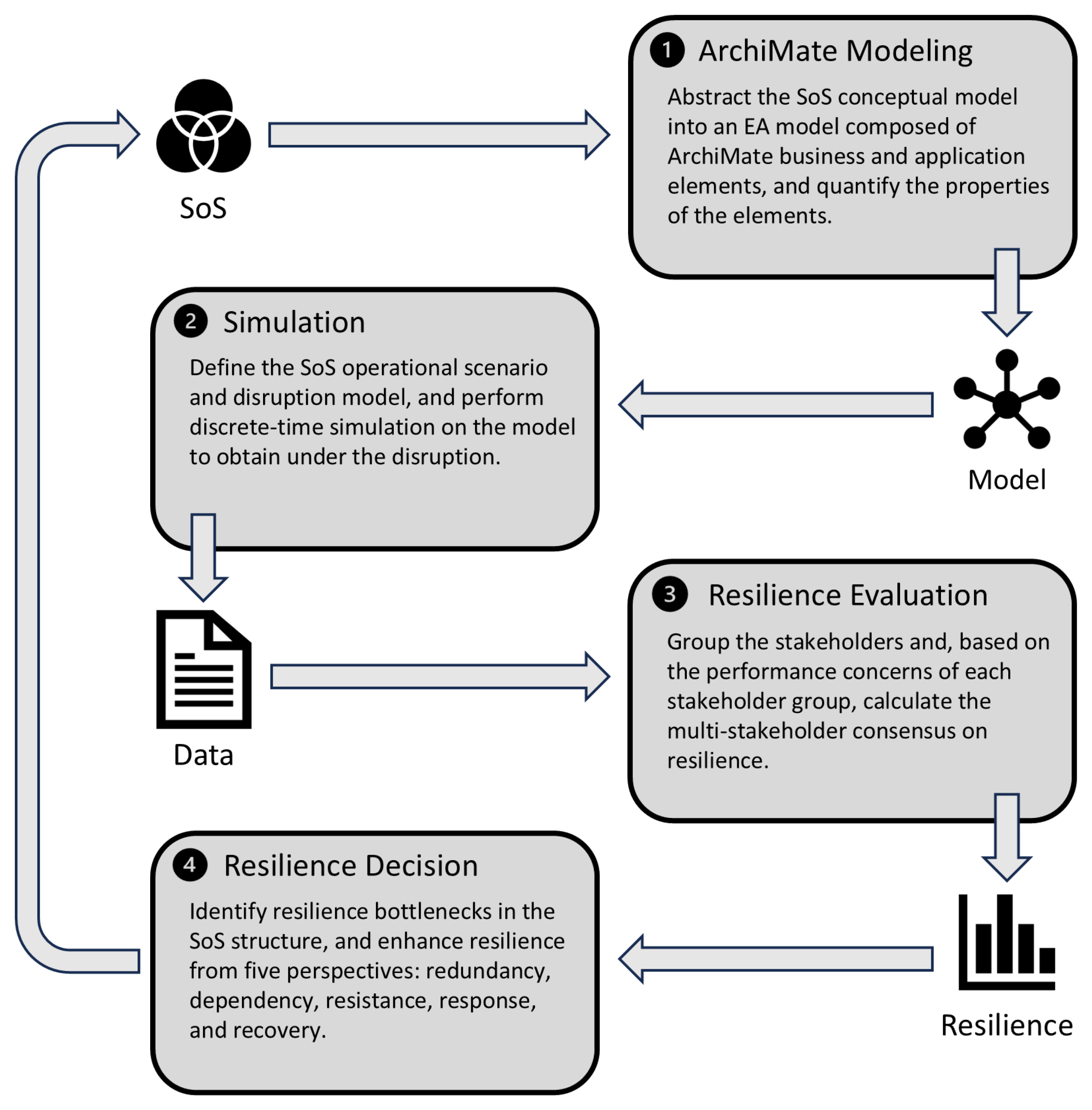
The proposed framework, as illustrated in Figure 1, consists of ArchiMate modeling, simulation, resilience evaluation, and resilience-informed decision making. This method has three key objectives: (1) to provide quantitative metrics for evaluating the resilience of the SoS, (2) to identify critical CS services, and (3) to offer recommendations for resilience-oriented design. In the SoS life cycle defined in ISO 21839 [62], the proposed framework facilitates resilience evaluation to support SoS design in the development phase. During the utilization phase, the proposed indicators remain applicable for resilience monitoring. When changes occur in the SoS environment or internal structure (e.g., legal amendments or the addition or removal of CSs), the SoS undergoes an iterative phase for resilience reevaluation and redesign.

Table 3. Definitions of identifiers in methodology section.

Identifiers	Definition
$ServingD$	The degree of dependency of the target of the serving relationship on the source.
$ServiceSC$	The number of user requests that can be fulfilled within a unit of time when external resources are abundant, subject only to the limitations of its own capabilities.
$ServiceRC$	The number of requests that can be fulfilled within a unit of time.
$ServiceD$	The steady-state demand (without any disruption) for CS service.
$Redundancy$	The redundancy of $ServiceSC$ which depends on dependability requirements of stakeholders when potential risk exist and is expressed in percentage form.
$ProcessRT$	The number of unit time required to complete the target SoS process in the absence of any disruptions.
$ProcessC$	The number of requests that can be fulfilled for the current process.
$UserGenerateSpeed$	The number of users generated per unit time in operational scenario.
$LowCapacity$	The lowest percentage of $ServiceSC$ after a disruption event occurs.
$RespondTime$	The unit time required to respond to a disruption event, from its occurrence to the initiation of recovery.
$RecoverTime$	The unit time required to recover to a disruption event, from the start of recovery to completion.
$t_0$	The start time of the simulation.
$t_1$	The time of the disruption occurrence.
$t_2$	The time of recovery initiation.
$t_3$	The time of recovery completion.
$UserPT$	The planned time for a user to request an SoS service.
$UserUT$	The actual used time for a user to request an SoS service.
$ServiceU$	The actual used capacity of a CS service.
$SoSR$	The number of users waiting in blocking queue.
$SoSW$	The number of users in running state.
R	The resilience indicator from the performance perspective.
$P\left(t\right)$	The performance curve under a disruption.
$P_0\left(t\right)$	The performance curve in the absence of disruptions.
$t_s$	The time of the disruption impact occurrence at SoS level.
$t_e$	The time of the SoS performance recovery completion.
$t_f$	The maximum value of $t_e$ among all CS disruptions.
$R_{wat}$	The SoS resilience indicator proposed by Watson.
$P^j$	The performance indicator of the stakeholder group j.
$R_i^j$	The SoS resilience indicator corresponding to $P^j$ when CS service i is disrupted.
$R_i^{*}$	The SoS resilience indicator when CS service i is disrupted.
$c_i^j$	The cost coefficient when stakeholder j reaches consensus.
${\varphi }^i$	The Shapley value, namely the resilience adjustment cost each stakeholder j must bear.
${\omega }_i$	The importance of $R_i^{*}$.
$R_{SoS}$	The SoS resilience indicator.

summarizes the variables and parameters introduced in this section along with their definitions.

3.1. ArchiMate Modeling

The EA tool ArchiMate offers a standardized modeling language for describing the operation of business processes, organizational structures, information flows, IT systems, and technical infrastructure. Built upon the TOGAF framework, it facilitates the end-to-end process from requirements analysis to organizational design and iterative improvements [63]. The process of modeling the SoS using the TOGAF framework includes the development of the SoS conceptual model, the business architecture model, the application architecture model, and the technology architecture model. This research employs its business architecture and application architecture to establish a description of the static structure of the SoS and the relationships among its CSs.

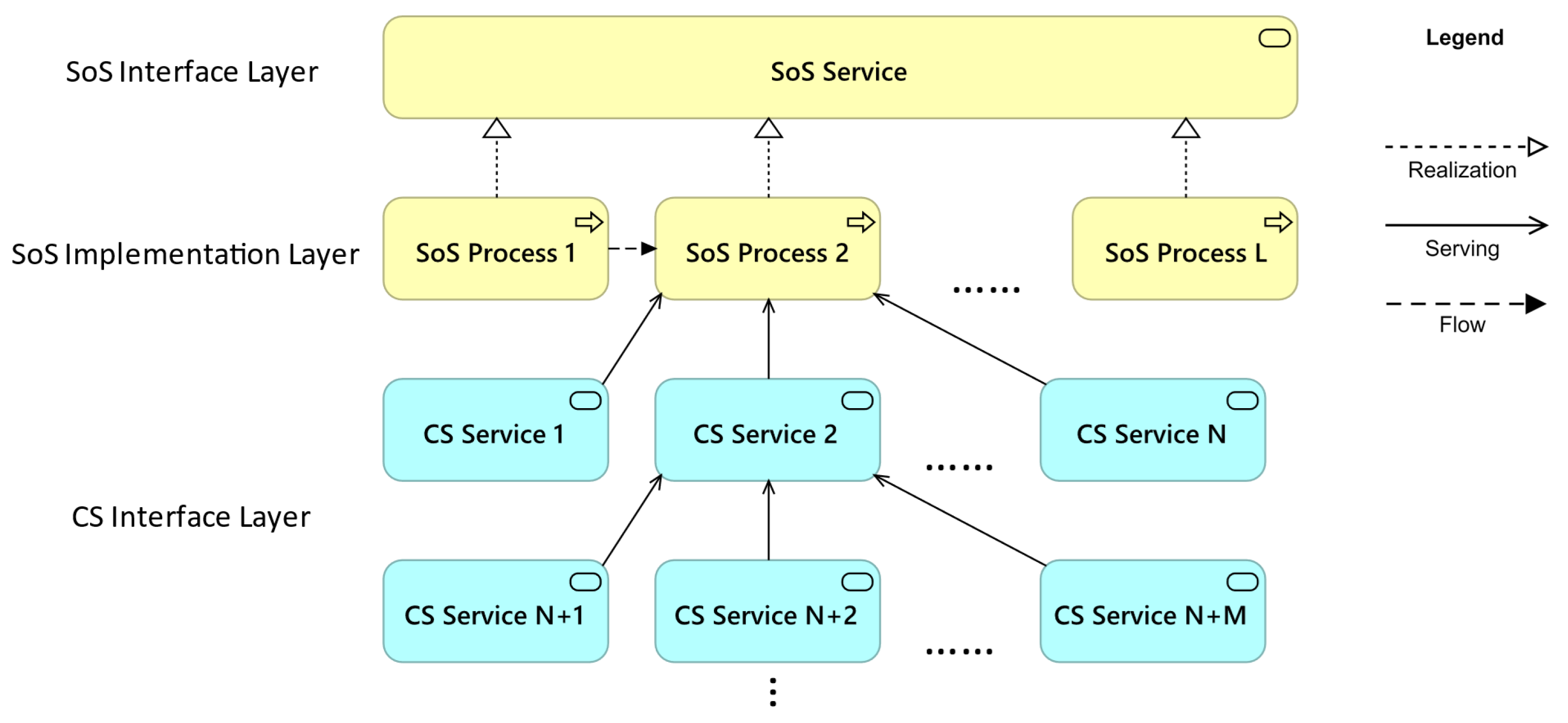
As illustrated in Figure 2, the real-world SoS is abstracted to the conceptual SoS architectures and matched with the concepts in the ArchiMate architecture. Three layers of ArchiMate’s core architecture: the business layer, application layer, and technology layer correspond to the SoS layer, the CS layer, and the system elements layer in the SoS architecture. Each layer consists of an interface layer that provides external services and an implementation layer that handles internal functionalities. This research focuses on modeling the relationship between CSs and SoS and therefore the internal composition of the CS function and their lower-level elements are omitted in the illustration, despite ArchiMate providing corresponding concepts to match them.

Table 4. Definitions of elements in ArchiMate [63].

Element	Definition
Business Service	Represents explicitly defined behavior that a business role, business actor, or business collaboration exposes to its environment.
Business Process	Represents a sequence of business behaviors that achieves a specific result, such as a defined set of products or business services.
Application Service	Represents an explicitly defined exposed application behavior.
Application Function	Represents automated behavior that can be performed by an application component.
Realization	Represents that an entity plays a critical role in the creation, achievement, sustenance, or operation of a more abstract entity.
Serving	Represents that an element provides its functionality to another element.
Flow	Represents transfer from one element to another.

provides definitions for key ArchiMate elements used in this study. The application layer defines the composition and interoperability of CSs, while the business layer expands the model to include additional stakeholders such as users, society, and SoS organizers. Unlike conventional models that focus solely on the flat, structural design of SoS, this model adopts a multidimensional perspective, capturing both its internal configuration and its broader socio-technical interactions.

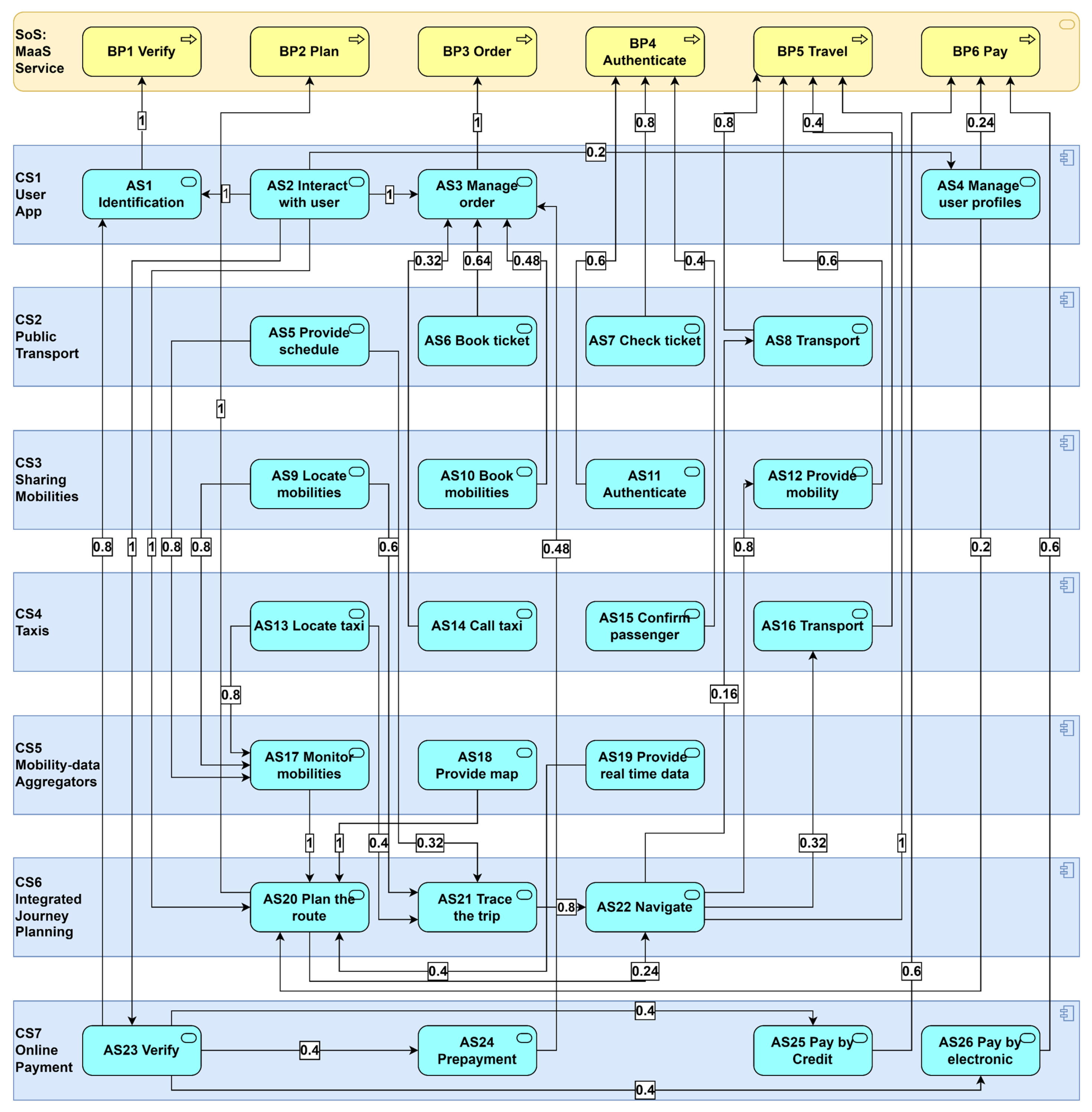
As illustrated in Figure 2, an SoS can be represented as an ArchiMate model, depicted in Figure 3. The model comprises four key elements: two nodes—the SoS process and CS service—and two directed edges representing the flow and serving relationships. The implementation of an SoS service follows a sequential execution of SoS processes, each requiring a certain amount of time to complete. When a specific SoS process is triggered, it utilizes the corresponding CS service, which may include information technology services (e.g., data provisioning), socio-technical services (e.g., transportation), or production and market services (e.g., inventory management). This operational logic serves as the foundation for the simulation detailed below. To enable quantitative simulation, key properties have been defined for these elements.

The flow relationship depicts the movement of users between the business processes and does not possess any inherent properties.

The serving relationship denotes that an element delivers its functionality to another element. It has a property, serving dependency ($ServingD$), which quantifies the degree of dependency of the target on the source in a serving relationship. This property is the answer to the following question: “How much source service is required when a target service is requested?”. This is defined as the product of request probability and absence tolerance, ranging from 0 to 1. Request probability quantifies the frequency at which the source service is requested when the target service is needed. Absence tolerance quantifies the degree to which the target service can tolerate the unavailability of the source service. They are quantified through a structured evaluation conducted among service-related stakeholders, using a quantitative rating table (see

Table 5. Evaluation of request probability and absence tolerance.

Requests Probability	Value	Absence Tolerance	Value
Never need	0	Would not regret its absence	0
Occasionally	0.2	Happy for its presence	0.2
Sometimes	0.4	Major absences are acceptable	0.4
Often	0.6	Moderate absence are acceptable	0.6
Frequently	0.8	Minor absence are acceptable	0.8
Always	1	Must have its presence	1

). For instance, if Service A frequently requires Service B, then the request probability of this serving relationship is 0.8. If Service A can tolerate a moderate absence from Service B, then the absence tolerance of this serving relationship is 0.6. Ultimately, the serving dependency ($ServingD$) value is the product of the two, resulting in 0.48. In other words, when there are 100 requests for Service A, 80 requests are made for Service B.

CS service represents an explicitly defined externally accessible application behavior provided by the CS. CS service has two properties: CS Service Self Capacity ($ServiceSC$) and CS Service Real Capacity ($ServiceRC$).

$ServiceSC$ quantifies the maximum number of user requests processed per unit time, assuming unlimited external resources and constrained solely by the system’s inherent capacity. $ServiceSC$ is formally defined in Equation (1).

$$ServiceSC\left(t\right)=ServiceD·\left(1+Redundancy\right)·Disruption\left(t\right)$$

(1)

$ServiceD$ represents the steady-state demand (in the absence of disruptions) for a CS service. This parameter ensures supply–demand equilibrium for services before disruptions occur. $Redundancy$ is determined by stakeholder-defined dependability requirements in the presence of potential CS risks and is expressed as a percentage. $Disruption\left(t\right)$ represents the impact of unexpected events on the performance of the CS service, quantified in percentage. Here, 0% signifies a complete loss of CS service performance, while 100% indicates no impact on CS service performance. The specific disruption model is detailed in Section 3.2.

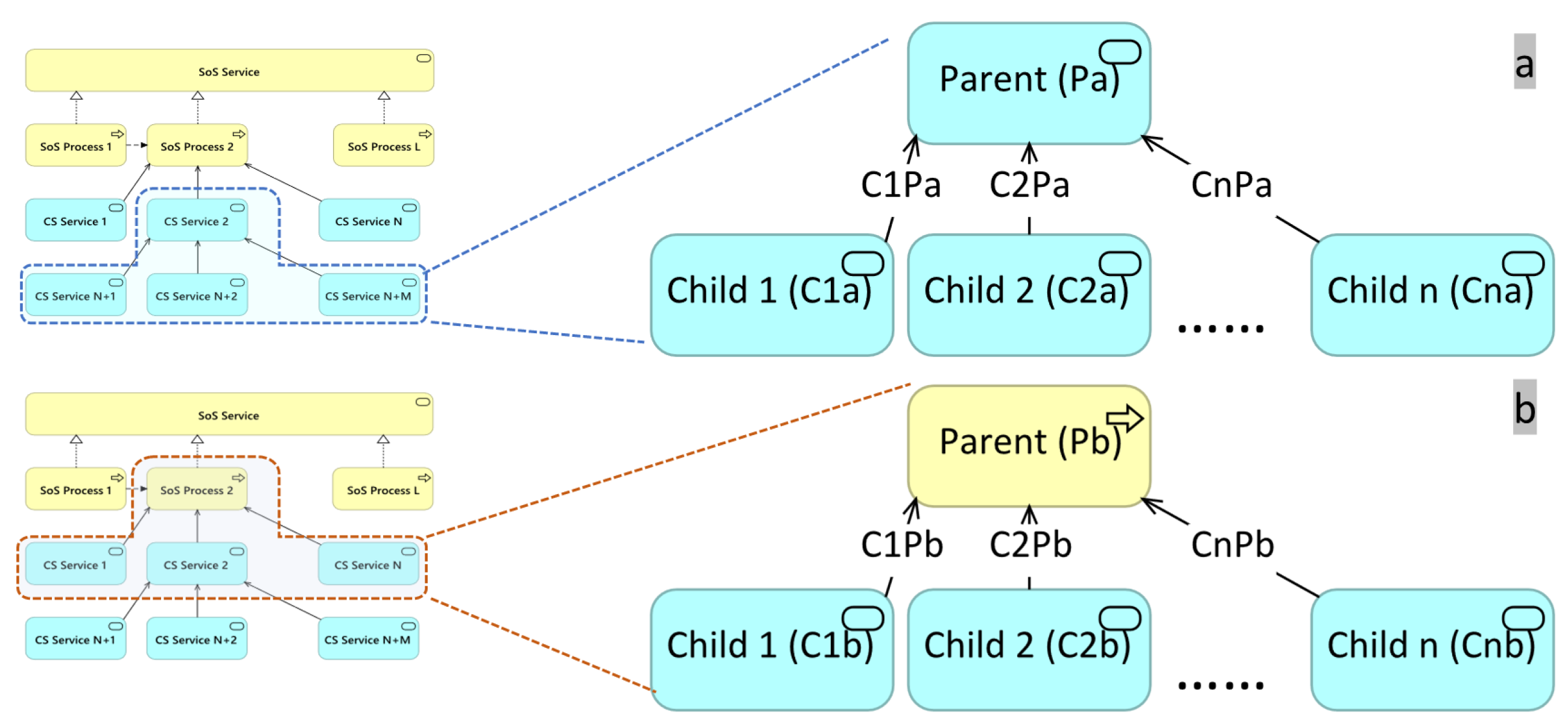
$ServiceRC$ quantifies the number of requests that can be fulfilled per unit time, determined by both its inherent capacity and the $ServiceRC$ of its dependent services. Figure 4a illustrates the scenario where a CS service relies on multiple CS services. The parent element $Pa$ depends on the child elements $C1a$, $C2a$,..., $Cna$, with the $ServingD$ of the serving relationships between them denoted as $C1Pa$, $C2Pa$,..., $CnPa$. $ServiceRC$ is formally defined in Equation (2). It indicates that $ServiceR{C}_P$ depends on the weakest point, which could be its own capacity, $ServiceS{C}_P$, or the service capacity of other dependencies, $ServiceR{C}_{C}n$.

$$\begin{array}{cc}\hfill ServiceR{C}_{P}a\left(t\right)=min& (ServiceS{C}_{P}a\left(t\right),{\displaystyle \frac{ServiceR{C}_{C2a}\left(t\right)}{Serving{D}_{C2Pa}}},\hfill \\ \hfill & {\displaystyle \frac{ServiceR{C}_{C1a}\left(t\right)}{Serving{D}_{C1Pa}}},\cdots ,{\displaystyle \frac{ServiceR{C}_{Cna}\left(t\right)}{Serving{D}_{CnPa}}})\hfill \end{array}$$

(2)

The SoS process represents a sequence of business behaviors that achieves a specific result, such as a defined set of products or business services. It has two properties, SoS process regular time ($ProcessRT$) and SoS process capacity ($ProcessC$).

$ProcessRT$ quantifies the time required to complete the target SoS process in the absence of disruptions. The property is derived from the average time taken to complete the SoS process.

$ProcessC$ quantifies the number of requests that can be fulfilled for the current process, determined by the $ServiceR{C}_{C}n$ of its dependent CS service. Figure 4b shows the scenario where a parent SoS process relies on multiple CS services. $ProcessC$ is determined by Equation (3). Similar to the computation of $ServiceRC$, Equation (3) signifies that $ProcessC$ depends on the weakest service capability among the CS services it relies on.

$$Process{C}_{P}b\left(t\right)=min\left({\displaystyle \frac{ServiceR{C}_{C1b}\left(t\right)}{Serving{D}_{C1Pb}}},\cdots ,{\displaystyle \frac{ServiceR{C}_{Cnb}\left(t\right)}{Serving{D}_{CnPb}}}\right)$$

(3)

3.2. Simulation

Resilience is highly context-dependent, influenced not only by the objective structure but also by the operational scenario and the nature of disruptive events [5]. Therefore, defining the operational scenario and disruption model is essential for resilience simulation.

Assumption of operational scenario: The user agent represents the source of service requests as well as the entity being served. Based on requirement analysis, the number of users generated per unit time ($UserGenerateSpeed$) can be determined. The generated agents simulate request behavior within the SoS, beginning with the initial SoS process and sequentially executing each subsequent process until completion. Agents are assumed to exist in three fixed states. If the SoS process is available, meaning that there is remaining capacity (defined as Equation (3)), then the agent will enter the running state and occupy the capacity at the current time step. Otherwise, the agent will enter the blocking state. Upon completion of an SoS process, the agent transitions to the ready state in preparation for the next SoS process. Given the configuration of $UserGenerateSpeed$, the variable $ServiceD$ (from Equation (1)) can be determined through steady-state simulation. In the steady-state simulation, disruptions are absent, ensuring a perfectly balanced supply and demand for services.

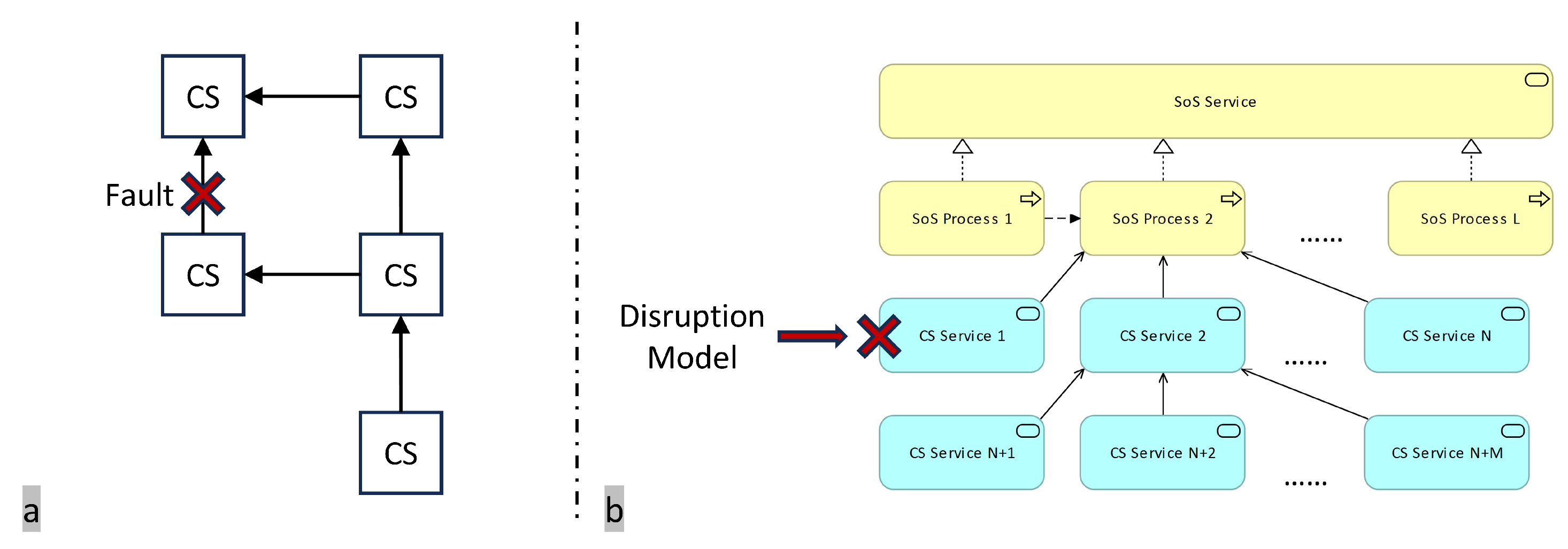
Assumption of disruption model: The disruption model captures the impact of disruptive events on CS services, as illustrated in Figure 5. Disruptive events can originate from any CS function or external environment. This study does not examine the causes of these events but rather focuses on their impact on CS services, as resilience primarily concerns how the failure of a CS function affects the integrity of the SoS. $t_0$ represents the time when the disruption occurs, and the CS service affected by the disruption immediately experiences a decrease in its capacity to a low level ($LowCapacity$), indicating the CS service’s resistance capability to disruption. $t_1$ denotes the start of the affected CS service’s recovery. The time interval between $t_0$ and $t_1$ reflects the CS service’s response capability to disruption, denoted as $RespondTime$. $t_2$ represents the time when the CS service fully recovers to its original capacity. The time interval between $t_1$ and $t_2$ quantifies the CS service’s recovery capability following a disruption, denoted as $RecoverTime$. The specific values for $LowCapacity$, $RespondTime$, and $RecoverTime$ need to be set in the simulation.

Generally, the parameters of the three aforementioned disruption models can be determined by the following three methods.

• Risk-informed method: If sufficient risk knowledge is available, then it can be acquired using various mature techniques, such as fault tree analysis. The parameters of the disruption model at the CS service level can then be determined through calculations or simulations at the system or component level. However, this approach may result in a reactive design paradigm, which is not conducive to macro-level resilient design [5].
• History-informed method: If ample historical data on CS service disruptions are available, then the parameters of the disruption model can be directly inferred from representative cases. However, this approach is often inadequate for predicting unknown scenarios.
• Requirement-informed method: Resilience engineering emphasizes the macro-level capacity to withstand disruptions. From this perspective, defining the parameters of the disruption model based on top–down requirements is a reasonable approach. This approach entails determining the extent of disruption that stakeholders expect the SoS to withstand while maintaining sufficient resilience and ensuring acceptable stakeholder losses. In this case, the disruption model serves as a benchmark similar to those used in software performance testing.

ArchiMate does not provide a dedicated simulation tool, but it does offer a scripting language called JArchi for model computation and batch processing. Based on JArchi, the author developed a discrete-time simulation program suitable for the model established in Section 3.1 (ArchiMate Version: 4.10.0, JArchi Version: 1.9.0) [64]. In the simulation, the state of the user agent and the properties of the CS change over time steps according to the equations in Section 3.1 and the settings in Section 3.2. The simulation progress is illustrated in Algorithm 1. Specifically, the disruption model is iteratively applied to each CS service to evaluate the resilience of the SoS, as represented by the loop in lines 3–15. During the simulation of a CS service disruption, user agents are instantiated at each time step (line 6), the SoS’s current performance is computed (line 7), the next state of each user agent is determined (lines 8–10), and the capacity utilization of each CS service is assessed (line 11).

The simulation output for each CS service disruption comprises the following elements: planned execution time ($UserPT$) for each user; actual execution time ($UserUT$) for each user; available service capacity ($ServiceRC$); service utilization ($ServiceU$) for each CS service; SoS process at each simulation time; the number of active users ($SoSR$) within the entire SoS; the number of queued users ($SoSW$) within the entire SoS.

Algorithm 1 Simulation for SoS MODEL.
Require: SoS Model (Topology and Properties)
Ensure: performance-related Data.
1:	Disruption Setting: $LowCapacity$, $RespondTime$, $RecoverTime$
2:	User Setting: $SimulationTotalTime$, $UserGenerateSpeed$,
3:	for $CS\_Service$ in SoS Model do
4:	Load Disruption to $CS\_Service$
5:	for i = 1,2,3...$SimulationTotalTime$ do
6:	Put number of $UserGenerateSpeed$ agents in AgentActiveArray.
7:	Traversal calculation of $ProcessC$ and $ServiceRC$.
8:	for $agent$ in ActiveAgentArray do
9:	Function: StateMachine($agent$)
10:	end for
11:	Traversal calculation of $ProcessU$ and $ServiceU$
12:	Store the data of time i
13:	end for
14:	Save the data of $CS\_Service$ in file format.
15:	end for

3.3. Resilience Evaluation

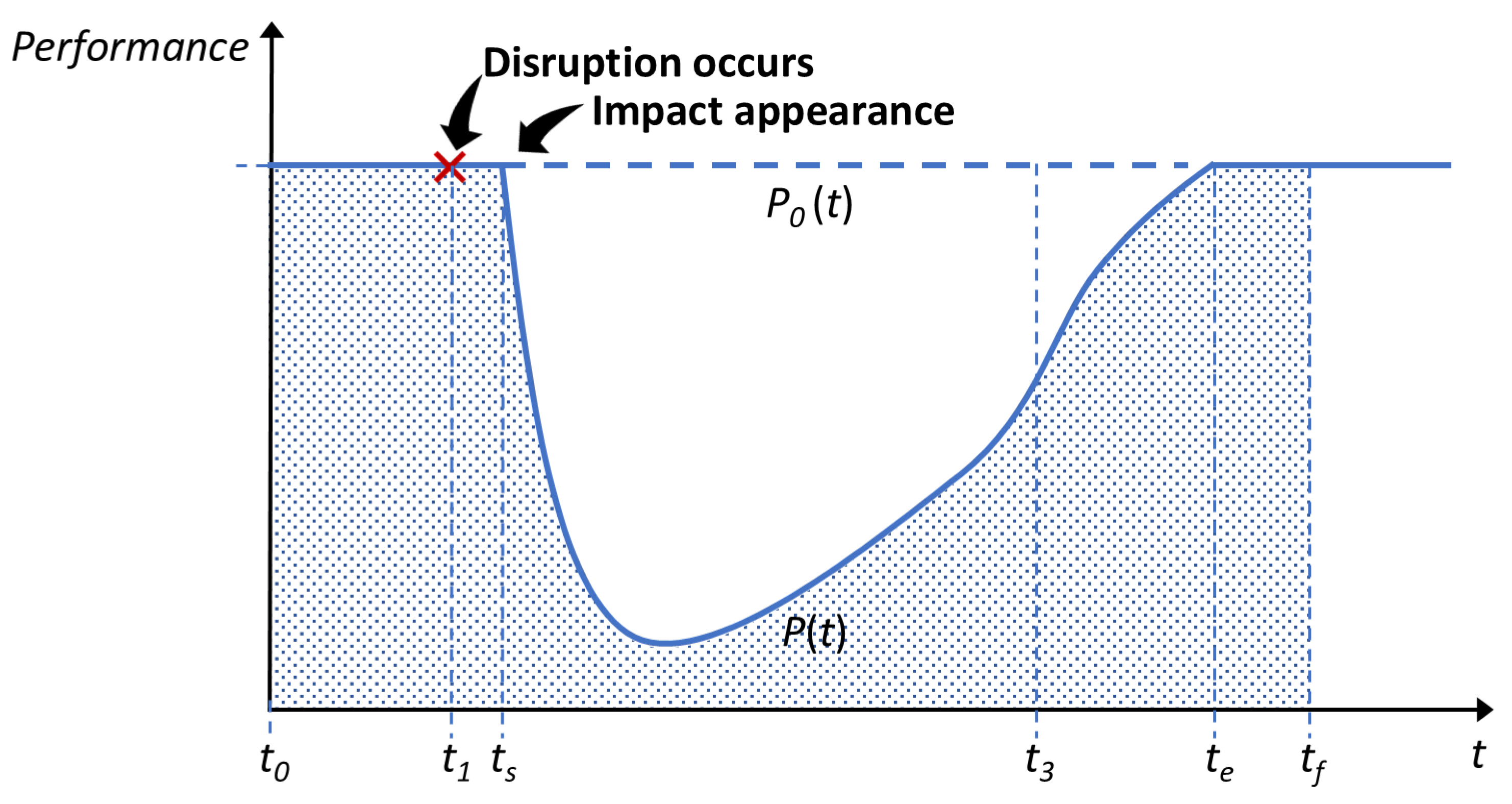
The performance method, which is currently the mainstream approach for resilience evaluation, employs a characteristic indicator as defined in Equation (4). Resilience is quantified based on the disrupted performance curve, $P\left(t\right)$, and the regular performance curve, $P_0\left(t\right)$ [61].

$$R={\displaystyle \frac{{\int }_{t_s}^{t_e}P\left(t\right)\mathrm{d}t}{{\int }_{t_s}^{t_e}{P}_0\left(t\right)\mathrm{d}t}}$$

(4)

In this equation, $t_s$ denotes the time at which the disruption impact becomes evident, while $t_e$ represents the duration required for the SoS to restore its regular performance following the disruption. Figure 6 illustrates the two performance curves defined in Equation (4).

Building on Equation (4), Watson proposed a method for evaluating the resilience of SoS, as formulated in Equation (5) [27]. He developed a physical flow graph model for the SoS, depicted in Figure 7a, where nodes represent CS and edges represent flow (e.g., energy flow within an ecological chain). By sequentially disrupting each individual edge (totaling k edges) and analyzing the corresponding performance curves, he derived the overall resilience of the SoS. Here, $T^{*}$ denotes the time required for full recovery.

$$R_{wat}={\displaystyle \frac{1}{k}}\sum _{fault=1}^k{\displaystyle \frac{{\int }^{T^{*}}P\left(t\right)\mathrm{d}t}{{\int }^{T^{*}}{P}_0\left(t\right)\mathrm{d}t}}$$

(5)

The study further explores this resilience definition from the perspective of the established ArchiMate model and a multistakeholder approach.

First, we introduce the disruption model as mentioned in Section 3.2. The term “fault” in Equation (5) denotes the disruption of an edge in the graphical structure, which implies the complete failure of the source CS. However, as a system, the CS is neither atomic nor strictly binary in terms of functionality—i.e., it is not either working or not working. Instead, it operates through three phases: disruption, response, and recovery. Therefore, we introduced the disruption model with parameters showing survival and recovery capability to simulate more detailed scenarios, as shown in Figure 7b. Resilience $R_i$ is defined in Equation (6), which quantifies the resilience of the SoS when CS service i experiences a disruption. In Figure 6, because $t_s$ and $t_e$ vary across different disruptions, we set $t_0$ as the starting time, assuming a uniform disruption occurrence time in the simulation, and define the maximum of all $t_e$ values as the end time $t_f$ to maintain consistent time intervals for all resilience computations.

$$R_i={\displaystyle \frac{{\int }_{t_0}^{t_f}{P}_i\left(t\right)\mathrm{d}t}{{\int }_{t_0}^{t_f}{P}_0\left(t\right)\mathrm{d}t}}$$

(6)

Second, we introduce multiple stakeholders. In Equation (5), performance is defined in a singular manner. This is more characteristic of general systems, where stakeholders typically have closer relationships and more aligned objectives. In contrast, stakeholders in a SoS are often diverse, decentralized, and concerned with broader societal impacts and interests, resulting in a more heterogeneous definition of performance. However, considering the performance objectives of all individual stakeholders is infeasible. A feasible approach is to group stakeholders with similar interests [65]. Based on stakeholder theory, the SoS should consider internal stakeholders who focus on profit, such as CS service providers and the SoS organizer, and external stakeholders who prioritize Quality of Service (QoS), namely users and society, since these four stakeholder groups play a crucial role in SoS decision making [66]. At the end of Section 3.2, some outputs of the simulation that can be used to calculate the performance indicators of each stakeholder group are mentioned, and we summarize them in

Table 6. Stakeholders’ interests and the simulation data related to these interests.

	Interests	Related Data
$P^{CS}$	CS profit	CS service capacity ($ServiceRC$) , capacity used ($ServiceU$)
$P^{SoS}$	SoS profit	SoS process capacity ($ProcessC$), capacity used ($ProcessU$)
$P^{User}$	Individual QoS	Order planned time ($UserPT$), used time ($UserUT$)
$P^{Soc}$	Overall QoS	Waiting population ($SoSW$) and running population ($SoSR$)

.

Using Equation (6), the resilience indicators corresponding to the above performance indicators are derived, denoted as $R_i^{CS}$, $R_i^{SoS}$, $R_i^{User}$, and $R_i^{Soc}$. The overall resilience indicator $R_i^{*}$ reflects the consensus among the four stakeholder groups. Equations (7) and (8) define a basic consensus process, where $ST$ denotes the set of the four stakeholder groups, and $c_i^j$ represents the cost incurred by the corresponding stakeholder group when adjusting their resilience evaluation to reach consensus. This parameter is determined based on loss estimation in accordance with real-world conditions. This optimization determines the overall resilience indicator $R_i^{*}$ by minimizing the total adjustment cost incurred by all stakeholder groups when aligning their individual resilience evaluations $R_i^j$ to a consensus value.

$$\begin{array}{cc}\hfill \underset{R_i^{*}}{min}\hspace{0.25em}& \sum _{j\in ST}{c}_i^j\left|R_i^{*}-R_i^j\right|,\hfill \end{array}$$

(7)

$$\begin{array}{cc}\hfill \mathrm{s}.\mathrm{t}.\hspace{0.25em}& R_i^{*}\in [0,1].\hfill \end{array}$$

(8)

The solution of this consensus process is not unique. To ensure fairness in consensus formation, we introduce the Shapley value from cooperative game theory. we construct a cooperative game model $G=〈ST,v〉$. The player set is the set $ST$. T$\left(T\in ST\right)$ means any coalition composed of members of $ST$. The characteristic function $v\left(T\right)$ equals the optimal value $l^T$ for Equations (9)–(11) below. Equation (9) identifies the most favorable solution to coalition T among the solutions of Equation (7), i.e., the one with the minimal total cost caused by adjustment for T. Therefore, an additional constraint (10) is introduced, ensuring that the sum of all stakeholders’ resilience evaluation adjustments equals the optimal value of Equation (7), noted as $l^{ST}$.

$$\begin{array}{cc}\hfill \underset{R_i^{*}}{min}\hspace{0.25em}& \sum _{j\in T}{c}_i^j\left|R_i^{*}-R_i^j\right|,\hfill \end{array}$$

(9)

$$\begin{array}{cc}\hfill \mathrm{s}.\mathrm{t}.\hspace{0.25em}& \sum _{j\in ST}{c}_i^j\left|R_i^{*}-R_i^j\right|=l^{ST},\hfill \end{array}$$

(10)

$$\begin{array}{cc}\hfill & R_i^{*}\in [0,1].\hfill \end{array}$$

(11)

The Shapley value distributes benefits and costs according to marginal contributions and satisfies several desirable axiomatic properties, such as efficiency, symmetry, linearity, and the null player condition, which guarantees fairness in the allocation process [67,68]. As defined in Equation (12), the Shapley value ${\varphi }^j$ assigned to stakeholder i is computed based on the characteristic function $v\left(T\right)$. It quantifies the resilience adjustment cost allocated to each stakeholder.

$$\begin{array}{cc}\hfill {\varphi }^j=& {\displaystyle \frac{1}{\left|ST\right|!}}\sum _{T\subseteq ST\setminus \left\{i\right\}}{\displaystyle \frac{\left|T\right|!\left(\right|ST|-|T|-1)!}{\left|ST\right|!}}\times \left[v(T\cup \{i\left\}\right)-v\left(T\right)\right].\hfill \end{array}$$

(12)

By incorporating the Shapley value ${\varphi }^j$ into the consensus process, the optimization problem formulated in Equations (13)–(15) determines the resilience evaluation $R_i^{*}$ by minimizing the total weighted adjustment cost across all stakeholder groups while ensuring that each stakeholder’s individual adjustment cost equals their allocated Shapley value ${\varphi }^j$, thereby maintaining a fair distribution of resilience adjustments.

$$\begin{array}{cc}\hfill \underset{R_i^{*}}{min}\hspace{0.25em}& \sum _{j\in ST}{c}_i^j\left|R_i^{*}-R_i^j\right|,\hfill \end{array}$$

(13)

$$\begin{array}{cc}\hfill \mathrm{s}.\mathrm{t}.\hspace{0.25em}& c_i^j\left|R_i^{*}-R_i^j\right|={\varphi }^j,\forall j\in ST,\hfill \end{array}$$

(14)

$$\begin{array}{cc}\hfill & R_i^{*}\in [0,1].\hfill \end{array}$$

(15)

Third, we introduce the importance coefficient. In Equation (5), the resilience of the SoS under each fault scenario is evaluated, and the overall resilience is computed as the average of these evaluations. This implies that disruptions with significant losses are given the same weight as those with minor losses. However, resilience refers to the capacity to withstand low-frequency, high-impact disruptions [5]. Therefore, the overall resilience indicator should account for the significance of critical CS services. Here, we introduce the coefficients ${\omega }_i$, as shown in Equation (16), to quantify the relative importance of each CS service. This implies that CS services with lower resilience $R_i^{*}$ are assigned higher importance weights, where m denotes the total number of CS services.

$${\omega }_i={\displaystyle \frac{1-R_i^{*}}{{\sum }_{i=1}^m\left(1-R_i^{*}\right)}}$$

(16)

The overall resilience of the SoS is defined as $R_{SoS}$ and shown in Equation (17).

$$R_{SoS}={\displaystyle \frac{1}{m}}\sum _{i=1}^m{\omega }_i{R}_i$$

(17)

3.4. Resilience Decision

The purpose of this section is to demonstrate the significance of the proposed resilience evaluation method, namely providing a basis for decision making in the SoS resilience designing phase. Three key questions arise in this phase:

• Q1: Among multiple SoS design options, which design option is preferable?
• Q2: Which CSs are the bottlenecks that need improvement when a design option lacks resilience?
• Q3: What measures should be taken based on identified bottlenecks?

For Q1, $R_{SoS}$ serves as an indicator for assessing the resilience of multiple design options, providing a quantitative basis for decision making.

For Q2, ${\omega }_i$ quantifies the criticality of CS service i. A larger ${\omega }_i$ value suggests that a disruption in CS service i would result in more significant losses for the SoS. This helps prioritize resilience measures by identifying critical CS services.

For Q3, first, it is important to distinguish reliability from resilience. Reliability focuses on the system by predicting and mitigating risk-related factors (e.g., probability of failure and impact). However, resilience is not about avoiding failure but ensuring system quality by monitoring and improving the system’s leading indicators (e.g., survival and recovery capability) [69]. Specifically, these indicators related to robustness, self-healing capability, redundancy, and decentralization [70].

Table 7. The leading indicators of resilience and corresponding improvement measurements on critical CS services.

Resilience Indicators	Corresponding Measurements
Robustness	Increase the LowCapacity
Self-healing capability	Decrease the RespondTime and RecoverTime
Redundancy	Increase the Redundancy
Decentralization	Reducing ServingD on critical CS services

shows the corresponding properties of these indicators in the SoS EA model established in this paper. Resilience engineers should consider the potential disruptions and prepare the corresponding properties of critical CS services during the SoS design phase and design monitoring mechanism to ensure the resilience of SoS during runtime.

4. Case Study: Mobility as a Service

4.1. MaaS Introduction

The definition of MaaS, along with the organizational structure (including processes and supplier integration) used in this section, refers to the Brussels MaaS trial report. The parameters in the model are only sample data derived from the assumptions in Section 3.2 [71]. MaaS is a seamless integration of mobility services and manages the provision of transport-related services, such as route planning, navigation, transportation, ticketing, and payment. Currently, the main operational mode of MaaS is the integration of existing mapping services, transportation companies, and payment companies. These companies operate independently and join MaaS through agreements to gain more profits through cooperation. Therefore, MaaS can be seen as an SoS, and the customers, MaaS organizers, integrated service providers, and society can be viewed as four stakeholder groups. MaaS is divided into six seamless business processes:

• Log in: MaaS verifies user identity and payment account authentication.
• Plan: An information integration process. MaaS provides users with travel options by integrating map data, vehicle availability, and transportation schedules.
• Order: A booking integration process. MaaS offers users a one-stop ticketing service by consolidating ticketing systems from various transportation platforms.
• Authenticate: MaaS verifies passengers’ identities upon boarding.
• Travel: A transportation integration process. MaaS combines various transportation modes to provide users with seamless travel and navigation services.
• Pay: A payment integration process. MaaS supports multiple payment methods and internally distributes revenue among different CSs.

The actual implementation of each business process involves multiple service providers, including transportation service providers, such as public transport, sharing mobility, and taxis, as well as comprehensive service providers, including integrated journey planning, mobility data aggregators, and online payment platforms. These providers are modeled as CSs to deliver services.

4.2. Method Implementation

4.2.1. Step 1: MaaS Modeling

The MaaS ArchiMate model, as depicted in Figure 8, has been developed based on the approach presented in Section 3.1. In this model, users sequentially trigger business processes (BP in the figure) within MaaS. Each business process depends on the support of multiple application services (AS in the figure) provided by CSs. The value assigned to the serving relationship in Figure 8 represents its parameter $ServingD$, which is empirically determined based on Table 5.

4.2.2. Step 2: MaaS Simulation

We have established a fundamental resilience evaluation scenario. In a given region’s MaaS, the demand is set at 20 user orders per unit of time. Each CS function provides a corresponding number of services based on this scenario, with an additional 20% redundancy to accommodate unforeseen events as per protocol. Furthermore, based on stakeholder requirements, MaaS must demonstrate sufficient resilience even when each CS function undergoes a certain level of disruption ($LowCapacity=20\%$, $RespondTime=15$, and $RecoverTime=30$). In this context, the model parameters serve as assumptions to illustrate the methodology; however, in practice, they can be determined through various methods, including risk analysis (e.g., applying Failure Modes and Effects Analysis (FMEA) to assess potential degradation of order service AS3 due to network attacks), historical data (e.g., analyzing statistical data on decreased performance of public transportation service AS8 caused by vehicle deceleration during heavy rain), and stakeholder requirements (e.g., ensuring service continuity even in the event of a complete failure of the credit card system, AS25). The parameter settings for this scenario are presented in

Table 8. Parameters and assumptions setting for MaaS simulation.

	Parameters	Value
Disruption model	$LowCapacity$	20%
	$RespondTime$	15
	$RecoverTime$	30
User agent	$UserGenerateSpeed$	20
CS service	$Redundancy$	20%

. If a CS service fails to meet demand after experiencing disruption, reinforcing the relevant SoS structure and enhancing the corresponding CS service properties becomes necessary. The simulation of the MaaS model was conducted using ArchiMate Version 4.10.0 and JArchi 1.1.0.

4.2.3. Step 3: MaaS Resilience Evaluation

The foundation for resilience evaluation lies in identifying performance indicators for the four stakeholder groups.

MaaS organizers, serving as decision-makers, designers, and investors, focus on the overall service capacity of the SoS. This capacity, defined as the maximum number of users that can be served, is determined by the sum of the service capacities of all business processes ($Process{C}_i$), as expressed in Equation (18).

$$P_{Organizer}=\sum _{i=1}^{6}Process{C}_i$$

(18)

CS providers enter into contracts with MaaS to offer their independent services and primarily focus on profitability. The utilization rate of CS services can, to some extent, reflect their turnover and expenses. Therefore, Equation (19), which represents the average utilization rate of all CS services, serves as the performance indicator for CS providers. The number ‘26’ denotes the total number of CS services in MaaS. The numerator represents the number of services being utilized, while the denominator represents the total number of services provided.

$$P_{Provider}={\displaystyle \frac{1}{26}}\sum _{i=1}^{26}{\displaystyle \frac{Service{U}_i}{ServiceS{C}_i}}$$

(19)

Users prioritize the punctuality of MaaS. For the stakeholder group of users, Equation (20), which represents the average punctuality rate, serves as their performance indicator. The set $U_t$ denotes users who complete their SoS service at time t. The numerator corresponds to the planned duration of the user’s itinerary, while the denominator represents the actual travel time.

$$P_{User}={\displaystyle \frac{1}{|U_t|}}\sum _{i\in U_t}{\displaystyle \frac{UserP{T}_i}{UserU{T}_i}}$$

(20)

For society, MaaS should strive to minimize congestion. The congestion rate, as defined in Equation (21), serves as the performance indicator. The denominator represents the total number of users, while the numerator denotes the number of users whose service is operating as scheduled.

$$P_{Society}\left(t\right)={\displaystyle \frac{SoSR\left(t\right)}{SoSR\left(t\right)+SoSW\left(t\right)}}$$

(21)

Based on the performance definitions of the four stakeholder groups, as given in Equations (18)–(21), the resilience evaluation for CS service i after experiencing a disruption can be determined using Equation (6). This yields the resilience indicators $R_i^{CS}$, $R_i^{SoS}$, $R_i^{User}$, and $R_i^{Soc}$. The results are presented in the first four columns of

Table 9. Resilience result and CS service importance ranking.

	SoS Organizer		CS Providers		User		Social		${\mathit{R}}_{\mathit{i}}^{*}$
	${\mathbf{R}}_{\mathbf{i}}^{\mathbf{SoS}}$	Rank	${\mathit{R}}_{\mathit{i}}^{\mathit{CS}}$	Rank	${\mathit{R}}_{\mathit{i}}^{\mathit{User}}$	Rank	${\mathit{R}}_{\mathit{i}}^{\mathit{Soc}}$	Rank	Value	${\mathit{\omega }}_{\mathit{i}}$
‘AS2’	0.9246	1	0.9644	19	0.8401	1	0.8339	1	0.8825	0.0501
‘AS4’	0.9362	2	0.9515	10	0.8465	3	0.8408	2	0.8910	0.0465
‘AS5’	0.9393	4	0.9566	13	0.8510	4	0.8465	4	0.8950	0.0448
‘AS23’	0.9860	15	0.9484	6	0.8445	2	0.8439	3	0.8960	0.0444
‘AS19’	0.9392	3	0.9515	9	0.8588	5	0.8467	5	0.8990	0.0431
‘AS9’	0.9394	5	0.9570	14	0.8602	6	0.8475	6	0.8995	0.0429
‘AS20’	0.9395	8	0.9492	8	0.8608	8	0.8481	10	0.9005	0.0425
‘AS17’	0.9395	6	0.9518	11	0.8608	9	0.8481	8	0.9005	0.0425
‘AS18’	0.9395	7	0.9518	12	0.8608	10	0.8481	9	0.9005	0.0425
‘AS13’	0.9395	9	0.9571	15	0.8607	7	0.8480	7	0.9005	0.0425
‘AS16’	0.9468	12	0.9651	20	0.8696	12	0.8578	13	0.9085	0.0391
‘AS12’	0.9468	13	0.9652	21	0.8702	14	0.8584	14	0.9085	0.0391
‘AS8’	0.9468	14	0.9652	22	0.8702	15	0.8584	15	0.9085	0.0391
‘AS22’	0.9467	11	0.9728	23	0.8696	13	0.8578	12	0.9085	0.0391
‘AS21’	0.9467	10	0.9753	24	0.8695	11	0.8578	11	0.9085	0.0391
‘AS1’	0.9964	24	0.9380	1	0.8879	22	0.8734	18	0.9130	0.0371
‘AS3’	0.9931	18	0.9460	2	0.8892	23	0.8774	21	0.9175	0.0352
‘AS10’	0.9931	16	0.9478	3	0.8875	20	0.8755	19	0.9180	0.0350
‘AS24’	0.9931	17	0.9478	4	0.8875	21	0.8755	20	0.9180	0.0350
‘AS6’	0.9931	19	0.9484	5	0.8895	24	0.8777	22	0.9190	0.0346
‘AS14’	0.9932	20	0.9485	7	0.8902	25	0.8784	23	0.9190	0.0346
‘AS11’	0.9962	21	0.9578	16	0.8821	16	0.8699	16	0.9200	0.0341
‘AS7’	0.9962	22	0.9584	17	0.8842	19	0.8722	17	0.9210	0.0337
‘AS15’	0.9964	23	0.9600	18	0.8922	26	0.8809	26	0.9260	0.0316
‘AS25’	0.9965	25	0.9961	25	0.8821	17	0.8800	24	0.9390	0.0260
‘AS26’	0.9965	26	0.9961	26	0.8821	18	0.8800	25	0.9390	0.0260
$R_{SoS}$: 0.9079

. The subcolumn labeled “Rank” indicates the ranking of CS services based on their importance from the perspective of the corresponding stakeholder group’s performance indicator.

Then, $R_i^{CS}$, $R_i^{SoS}$, $R_i^{User}$, and $R_i^{Soc}$ are used as inputs to the consensus model based on cooperative game theory, as defined in Equations (7)–(15). The consensus resilience $R_i^{*}$ between all stakeholders for the disruption is calculated, with the results recorded in the subcolumn ’Value’ of $R_i^{*}$ in Table 8. The ${\omega }_i$ subcolumn of $R_i^{*}$ represents the importance weight of each CS service, derived using Equation (16). Finally, the consensus evaluation of all disturbances and their corresponding weights is used as input to Equation (17), resulting in a MaaS resilience value of 0.9079.

In this dataset, the resilience evaluation rankings of $R_i^{CS}$ differ significantly from those of other stakeholder groups. To further illustrate the divergence in resilience assessments among different stakeholder groups, this study calculates the Spearman correlation coefficient for the resilience data in Table 9, with the results presented in Figure 9. At a significance level of $\alpha =0.005$, the resilience evaluations by SoS organizers, users, and social stakeholders exhibit a significant positive correlation with one another. However, the evaluations by CS providers do not demonstrate a linear correlation with those of other stakeholders. This indicates a discrepancy between CS providers and other stakeholder groups in terms of resilience assessment. The primary reason for this divergence lies in the performance metric used for CS providers, which is service utilization and incorporates redundancy costs. In contrast, the performance metrics for other stakeholder groups do not account for resilience cost considerations.

4.2.4. Step 4: MaaS Resilience Decision

In response to the three questions posed in Section 3.4, the answers are as follows:

A1: The resilience of the MaaS model was evaluated to be 0.9079. This metric can be compared with other models to assess its relative superiority or inferiority.

A2: In Table 9, CS services are ranked in descending order of ${\omega }_i$, highlighting the relative importance of each CS service. “AS2 Interact with user” is identified as the most critical CS service in the MaaS model and should be prioritized for resilience enhancement. If, after improvement, the resilience still fails to meet stakeholder requirements, further reinforcement should be carried out based on the updated rankings.

A3: To enhance the resilience of the MaaS model, the following measures based on Table 7 are applied as examples to the critical CS service “AS2 Interact with user.” The term “Original” represents the state of MaaS before any improvements were implemented.

• Original: MaaS before any improvements and parameters set as Table 8.
• Method1: $Redundancy$ was increased from 20% to 50% by scaling up servers.
• Method2: $ServingD$ of the relationship relied on ’AS2’ was reduced 25% by increasing local servers.
• Method 3: $RespondTime$ was reduced from 15 to 9 by implementing network congestion monitoring and attack detection mechanisms.
• Method4: $RecoverTime$ was reduced from 30 to 15 by team security skills training.
• Method5: $LowCapacity$ was increased from 20% to 30% by adding firewalls.

The improvement results are presented in

Table 10. SoS resilience after enhancing AS2 using the five methods.

AS2	SoS Organizer	CS Providers	User	Social	${\mathit{R}}_2$
					Value	Rank
CG	0.9246	0.9644	0.8401	0.8339	0.8825	1
Method1	0.9374	0.9697	0.8903	0.8855	0.9135	16
Method2	0.9413	0.9722	0.8997	0.8952	0.9205	22
Method3	0.9400	0.9720	0.8861	0.8813	0.9130	15
Method4	0.9437	0.9715	0.8902	0.8851	0.9170	16
Method5	0.9342	0.9704	0.8707	0.8654	0.9025	10

. Methods 1 through 5 all contributed to enhancing SoS resilience and lowering the importance ranking of AS2. Furthermore, we conducted a one-at-a-time sensitivity analysis on the five parameters corresponding to the proposed measures. The results are shown in Figure 10. Initially, the sensitivity of the proposed resilience indicator to all five parameter changes offers preliminary evidence of its conceptual soundness. More specifically, as for the parameter $Redundancy$, introducing redundancy at earlier stages yields a more pronounced improvement in resilience. However, as redundancy continues to increase, the marginal benefits gradually diminish, ultimately stabilizing into a steady linear relationship between redundancy increments and resilience gains. Reducing the dependency on AS2, represented by the parameter $ServingD$, results in a linear improvement in resilience. When AS2 is no longer relied upon by the SoS, disruptions occurring within AS2 have minimal impact on the overall performance of the SoS. Similarly, the three parameters related to the disruption model—$RespondTime$, $RecoverTime$, and $LowCapacity$—exhibit a linear relationship with the resilience $R_2$ of AS2 after experiencing a disruption. Specifically, reducing $RespondTime$ and $RecoverTime$, as well as increasing $LowCapacity$, consistently improves resilience. This is because variations in these parameters under the disruption model are linearly associated with performance losses. It should be noted, however, that evaluating the effectiveness of resilience measures requires consideration of additional factors such as cost, feasibility, and legal constraints. Therefore, future research could incorporate these aspects, implement multi-parameter sensitivity analysis and explore more concrete resilience-enhancing decisions.

5. Conclusions

The approach proposed in this study enables the quantitative evaluation of SoS resilience, with the evaluation outcomes serving as a basis for SoS design. Firstly, the proposed SoS model, based on ArchiMate, facilitates communication among stakeholders and enhances the comprehension of non-specialist stakeholders. Secondly, the introduced quantified ArchiMate model and simulation assist engineers in testing resilience during the design phase. Finally, the SoS performance is evaluated from a multistakeholder perspective, incorporating the viewpoints of users, SoS organizers, CS providers, and society to ensure a comprehensive assessment of resilience.

MaaS was implemented as a case study to demonstrate the proposed resilience evaluation approach. The evaluation identified key CS services within MaaS and highlighted potential improvement directions. Enhancing MaaS resilience metrics can be achieved by strengthening the robustness, redundancy, and decentralization of its critical services. Furthermore, constructing a diverse, flattened, and low-coupling MaaS architecture can help balance resilience costs among stakeholders, further contributing to resilience enhancement. However, additional research is required to further analyze and identify specific resilience measures.

Building upon this foundation, further development is needed to establish a systematic approach for SoS resilience design. For instance, specific methodologies are required for deriving disruption models from risk analysis, historical data, and stakeholder requirements; dynamic modeling techniques for structural adaptation, including the introduction or decommissioning of CS services; ways of ensuring resilience during the operational phase of the SoS lifecycle and what measures can be taken when inconsistencies with the original design arise; modeling emergent behaviors through the inclusion of constituent system and user agents, enriched state variability, stochastic factors, and dynamic relationships. Finally, a critical need remains for further validation of the proposed method through its application to a broader range of real-world SoS instances, particularly in comparison with conventional dependability design methodologies.