Abstract
This study focuses on estimating transportation system-related emissions in CO2 eq., considering several socioeconomic and energy- and transportation-related input variables. The proposed approach incorporates artificial neural networks, machine learning, and deep learning algorithms. The case of Turkey was considered as an example. Model performance was evaluated using a dataset of Turkey, and future projections were made based on scenario analysis compatible with Turkey’s climate change mitigation strategies. This study also adopted a transportation type-based analysis, exploring the role of Turkey’s road, air, marine, and rail transportation systems. The findings of this study indicate that the aforementioned models can be effectively implemented to predict transport emissions, concluding that they have valuable and practical applications in this field.
1. Introduction
The increase in global consciousness regarding environmental issues and pollution has positioned models of environmental indicators and future projections as pivotal strategic instruments. Climate change is one of the most significant environmental issues at present. Greenhouse gas (GHG) emissions are key indicators of climate change. GHGs comprise carbon dioxide (CO2), methane (CH4), nitrous oxide (N2O), and fluorinated gases. Aggregate emissions can be articulated in terms of CO2 equivalents [1]. Transport is acknowledged as a key enabler of global trade and development. As with other economic sectors, the transport sector encounters considerable challenges in the context of climate change, specifically the need to reduce its carbon emissions [2], as it has been identified as one of the three top global contributors to CO2 emissions. In 2022, total transport emissions exhibited an increase of 2.1%, which was predominantly driven by growth in advanced economies. It is worth noting that this increase would have been more pronounced in the absence of the accelerated adoption of low-carbon vehicles [3]. On a global scale, although there has been some progress in recent years towards the decarbonization of road transport, particularly in urban transport, the decarbonization process is still in its initial stages for road freight, shipping, and aviation [2].
Effectively adapting to climate risk in the transport sector can be facilitated by integrating risk assessment and adaptation strategy planning into national adaptation plans and processes. This is crucial for the implementation of international agreements, such as the Paris Agreement [4]. In accordance with the Paris Agreement, parties are required to submit Nationally Determined Contributions (NDCs) to the United Nations Framework Convention on Climate Change (UNFCCC) secretariat every five years. Turkey has committed to reduce its GHG emissions by 41% compared to the baseline scenario by 2030. Turkey’s updated NDC is economy-wide and includes comprehensive mitigation and adaptation actions, as well as tools of implementation [5]. According to the Turkish Statistics Institute (TurkStat)’s GHG inventory data, Turkey’s total GHG emissions were 564.4 million tonnes (Mt) of CO2 eq., and transport emissions accounted for 16.2% of the total GHG emissions in 2021. Of these transport-related emissions, 94.8%, 3.1%, 1.2%, and 0.4% stem from road, air, marine, and rail transport, respectively, and 0.4% are due to other modes of transport. As of the end of 2022, 36.9% of registered cars were fueled with diesel, 35.1% with LPG, and 26.8% with gasoline, while 1.0% were electric or hybrid vehicles [6]. In 2023, Turkey published its Climate Change Mitigation Strategy and Action Plan for the 2024–2030 period. The development of future projections and prediction models in alignment with this strategy and action plan is anticipated to contribute substantially to our understanding of climate change dynamics in the region. Taking into account the importance of forecasting GHG or CO2 emissions, researchers have employed a range of methodologies [7], including grey modeling, statistical models, machine learning, and deep learning algorithms. The following concise overview provides a summary of some of these studies.
Lu et al. [8] adopted a grey model to predict the development trend of energy consumption and CO2 emissions in the road transport sector in Taiwan for the 2007–2025 period and investigated a range of economic growth scenarios. Kazancoglu et al. [9] used grey prediction to estimate GHG emissions from various road transportation vehicles across the European Union (EU) and in four individual EU countries. They also recommended policies aimed at reducing GHG emissions from road transportation at both the country level and for the entire EU. Huang et al. [10] developed a nonlinear multivariate grey model to predict carbon emissions from the transportation sector in China, the USA, and Japan. The gross domestic product (GDP), total energy consumption in the transportation sector, and population input variables were used in the proposed model.
Yagcitekin et al. [11] evaluated a transition in transportation to electrically driven vehicles in terms of CO2 emissions and energy requirements for Istanbul, Turkey. They adopted a radial basis function network to estimate the annual total electric energy consumption. Li et al. [12] employed ordinary least squares regression, support vector machine, and gradient boosting regression to predict the CO2 emissions of the transportation sector. The study incorporated both socioeconomic and transportation factors as features. Abdulmalik and Srivastava [13] studied the prediction of transportation-based CO2 emissions in Canada using artificial neural network, support vector machine, deep neural network, decision tree regressor, and gradient boost regressor methods. Data features pertaining to vehicle registration and the fuel consumption rating were utilized as independent variables. Emami Javanmard et al. [14] built an integrated framework that combines multi-objective mathematical modeling and machine learning algorithms, including the autoregressive integrated moving average, seasonal autoregressive integrated moving average, and support vector machines. The study predicted energy demand and CO2 emissions in the Canadian transport sector and investigated the impacts of energy resource types. Qiao et al. [15] proposed a multi-stage forecasting framework with the objectives of enhancing the accuracy of machine learning and deep learning models used and elucidating the relationship between predictions and influential features. They employed data from the United Kingdom’s transportation sector, integrating socioeconomic and transportation- and energy-related features. Temizçeri and Kara [16] studied a green intermodal transportation planning problem and developed a bi-objective mathematical model to solve the problem. To forecast transportation-based CO2 emissions, multiple linear regression, support vector regression, decision tree, and random forest algorithms were adopted and integrated with the mathematical model. Çınarer et al. [17] employed a multi-layer perceptron, extreme gradient boosting, and a support vector machine to predict transportation-related CO2 emissions in Turkey. Scenarios were defined and evaluated through the generation of disparate clusters among the designated input variables of energy consumption, vehicle kilometers, population, year, and GDP per capita.
Ratanavaraha and Jomnonkwao [18] forecasted CO2 emissions originating from the energy consumption of the Thai transportation sector. They utilized log-linear regression, path analysis, time-series, and curve estimation techniques, considering the population, GDP, and number of small, medium, and large registered vehicles as independent variables. Alhindawi et al. [19] used vehicle-kilometers by mode and the number of vehicles from road transport data to construct multi-variate regression and double-exponential smoothing approaches to estimate GHG emissions from road transportation. Isik et al. [20] employed the logarithmic mean Divisia index method to analyze and demonstrate the impact of various factors on CO2 emissions within Turkey’s transportation sector from 2000 to 2017. Lu et al. [21] performed an analysis to project the future trajectory of energy consumption and CO2 emissions in the context of road transportation in China. To this end, a Bayesian structural equation model was built to demonstrate the relationships between the total demand, structural characteristics, and technological advancements as pivotal factors influencing the road transportation system. Zhu et al. [22] projected CO2 emissions originating from the transportation sector in Shanghai, China through establishing an extended stochastic impact by regression on population, affluence, and technology model. The model extension expanded the three original variables (population, affluence, and technology) of the model to a total of six. These variables included population size, passenger turnover, GDP per capita, transportation intensity, energy intensity, and energy structure. Chang et al. [23] assessed emission reduction policies through a scenario analysis in Taiwan. CO2 emissions were modeled based on energy consumption and emission factors for various types of motor vehicles. Energy consumption was modeled using the number of registered vehicles, average distance traveled, and energy consumption per kilometer traveled.
As can be seen from the above overview of studies predicting the GHG or CO2 emissions of transport systems, many researchers have contributed to the literature using a variety of approaches. Given the distinct characteristics of transport systems in different countries, country-specific analyses have generally been performed. A variety of assessments have been conducted to analyze emission reduction policies in Turkey and numerous other countries. Even though there have been a number of studies on GHG emissions in Turkey’s transportation system, the dynamic nature of this sector means that regular updates and refined estimations are relevant and essential. Rapid growth in transport demand, changes in vehicle fleet and fuel mixes, new technologies (e.g., electric vehicles, hybrid vehicles), and evolving national policies indicate a continued need for new contributions.
Based on the literature review, existing research on predicting transportation-related CO2 emissions has a number of limitations. Many models primarily focus on single-mode transportation analysis, often emphasizing road transport without considering the interactions between multiple transport modes such as rail, air, and marine transport. Furthermore, while machine learning and statistical models have been widely applied, few studies have integrated multiple advanced techniques to enhance prediction accuracy and interpretability. Finally, few researchers have addressed scenario-based future projections by incorporating possible future technological developments and policy changes. This study addresses these gaps through the integration of multiple advanced algorithms to enhance model adaptability, conducting a comprehensive multi-mode transportation analysis to better capture system dynamics and incorporating scenario-based future projections to improve predictive accuracy and policy relevance.
This study presents a comprehensive approach to estimating transportation system-based emissions in CO2 eq., considering several socioeconomic and energy- and transportation-related input variables. The proposed approach incorporates artificial neural networks, machine learning, and deep learning algorithms. Taking Turkey as an example, algorithm performance is evaluated using a dataset Turkey. Although a number of studies have examined the context of Turkey, the present study develops a prediction approach for transportation system-sourced emissions based on ridge regression, support vector machine, and random forest algorithms, artificial neural networks, and long short-term memory networks. The models utilize multiple input variables regarding the output of transportation system emissions. The selection of models was based on their proven efficacy in the existing literature. Given the analysis of multiple datasets characterized by distinct properties, a range of models were employed to ensure the investigation was comprehensive. This study also employs a transportation type-based analysis that investigates the contributions of Turkey’s road, air, marine, and rail transportation systems. To the best of the authors’ knowledge, there have been limited studies conducted on transportation type-based emissions analysis considering a range of input variables with the adopted algorithms.
The remainder of this study is structured as follows. Section 2 provides the theoretical framework of the methodology and models employed. Section 3 defines the dataset from the case country. Section 4 presents a comprehensive overview of the studied data characteristics, experimental results, discussion, and scenario-based future projections. Finally, conclusions are provided in Section 5.
2. Materials and Methods
2.1. Ridge Regression
Ridge regression is a regularization technique employed to stabilize regression models in cases of multicollinearity. This method reduces predictor coefficients to reduce the risk of overfitting and achieve better generalization performance [24]. Ridge regularization introduces a penalty term to the loss function of linear models. This penalty is employed to promote the model’s capacity for achieving equilibrium between minimizing error and preserving the regression coefficient vector, denoted β, at a minimal magnitude, as shown in Equation (1).
refers the actual value or target/dependent variable, and denotes the independent or predictor variable. The parameter governs the trade-off between the fit of the data and the complexity of the model [25,26].
2.2. Support Vector Machine
The support vector machine is a machine learning method with a foundation in statistical learning theory; it is employed for problems of classification and regression. The use of this approach provides numerous benefits in the domain of nonlinear and high-dimensional pattern recognition problems. Support vector regression is a prediction approach based on a support vector machine that seeks to identify the optimal hyperplane such that the total deviation of all sample points from the hyperplane is minimized [27]. The regression equation f(x) is calculated according to Equation (2) [28]:
w and b indicate weight and bias, respectively. is a nonlinear function used to transform input data from low to high dimensional space. Next, the regression equation is presented as an optimization problem, as demonstrated in Equations (3) and (4) [28]:
xi and yi denote the input and output variables, respectively; C refers the regularization parameter that describes the trade-off between the flatness of f(x) and the loss function; and are slack variables [29]. The subsequent reformulation of the optimization problem as a dual optimization problem, utilizing the Lagrange multiplier method, facilitates the derivation of the nonlinear function, as presented in Equation (5).
where denotes the kernel function, and are Lagrangian multipliers [29]. The selection of the kernel function is pivotal in determining the efficacy of the method with regard to learning performance. The most frequently employed kernel functions are the linear, polynomial, and radial basis functions [28].
2.3. Random Forest
The random forest technique adopts the ensemble learning approach to regression. The technique generates a multitude of decision trees, the number of which often reaches the thousands. These decision trees function as independent regression functions, and the final output of the random forest regression is derived as the average of the outputs of all individual decision trees [29,30]. A decision tree is a hierarchical representation of if–then rules. Each decision tree consists of nodes (decision rules) and leaves (decisions). Before constructing a tree, it is imperative to ascertain the minimum number of samples required for node splitting and the maximum depth of the tree [31]. The random forest model has frequently been indicated to demonstrate a high level of performance in practical applications as an ensemble learning methodology [32].
2.4. Long Short-Term Memory
Long short-term memory (LSTM), a deep learning model, is a type of recurrent neural network architecture that is widely used, especially in time-series data and sequential data analysis. The development of LSTM was motivated by the observation of vanishing gradient problem in classical recurrent neural networks. LSTM uses a special cell structure to learn long-term dependencies, and thanks to this structure, it effectively manages both short- and long-term memories [33].
LSTM comprises three principal gates: forgetting, input, and output gates. The function of the forgetting gate is to determine degree to which previous information is to be disregarded [15]. The mathematical representation of the forgetting gate is given in Equation (6).
are the weighting metrics and bias vectors, respectively. is the activation function, which is defined as a sigmoid function. refers to the concatenation of the previous hidden state and the current input. The input gate and a tanh layer are improved to control new information stored in the cell. This is expressed mathematically in Equations (7) and (8).
is the activation function, which is defined as a hyperbolic tangent function. The cell state is given in Equation (9).
Finally, the output gate determines what information will be transferred to the output, which is given in Equations (10) and (11).
In Equations (7)–(11), is a hidden state; , and are the recurrent weighting metrics; and the bias vectors [15,34].
2.5. Artificial Neural Networks
An artificial neural network (ANN) is a mathematical model inspired by the structure of interconnected human brain cells. The most commonly used type of ANN is the feedforward multi-layer structure, which consists of an input layer, one or more hidden layers, and an output layer [35]. It is important to note that each of these layers performs a separate function. Initial data are received by the input layer. These inputs are processed by hidden layers that use weighted connections and activation functions to reveal nonlinearities. The final result or prediction is produced by the output layer [36].
The total input signal can be given as the weighted sum of the inputs, as in Equation (12).
where is the total input value, is the -th input, is the weight of the -th input, and is the bias term [37]. The total value is passed through an activation function. Sigmoid, ReLU, and tanh functions are well-known activation functions, the formulations of which are provided in Equations (13)–(15).
These outputs are used as the input of the next layer to produce the final result or prediction [35,38].
In order to enhance the performance of an ANN, the following factors are selected for consideration: the type of training algorithm, number of hidden layers, number of neurons in the hidden layers, and activation functions [36].
2.6. Performance Analysis
To analyze performance of the models, this study employed five of the most frequently used performance metrics, the mean square error (MSE), mean absolute error (MAE), root mean square error (RMSE), mean absolute percentage error (MAPE), and determination coefficient (R2), provided in Table 1. In the formulae below, refers to the actual value, denotes the predicted value, and n shows the total number of data points.

Table 1.
Definition of performance metrics.
It is evident that smaller values of the MSE, MAE, RMSE, and MAPE (i.e., closer to 0) show superior forecasting capability. The R2 ranges from 0 to 1, with higher values indicating greater accuracy in forecasting models [41]. Figure 1 illustrates the forecasting system developed in this study.
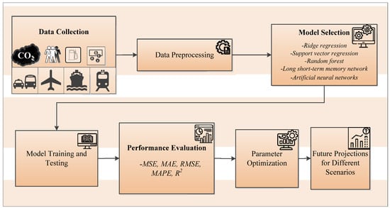
Figure 1.
Study framework.
3. Dataset
The dataset includes a range of socioeconomic and energy- and transportation-related input variables. The output variables encompass both the total annual transportation emissions and those emissions originating from road, air, marine, and rail transport modes, which were also designated as output variables. While socioeconomic input variables comprise the population and GDP per capita, energy-related input variables comprise the total final energy consumed by transportation systems and final transportation type-based energy consumption. Transportation-related input variables include both total and transportation type-based freight and passenger transportations. In addition, in road transport, the number of road motor vehicles, the number of electric and hybrid cars, and the weighted average daily traffic inputs are employed. Finally, electrified and non-electrified railway tracks were utilized in the rail transport dataset. The datasets considered within the scope of this study are summarized in Table 2. To demonstrate the composition of transport systems in Turkey, an analysis of freight transport rates within Turkey’s transportation systems revealed that in 2021, 92.47%, 3.36%, 4.16%, and 0.01% of freight was transported by road, marine, rail, and air transport, respectively. In the context of passenger transport, 92.8% of passengers were conveyed by road, 0.2% by marine, 0.6% by rail, and 6.4% by air.
Table 2.
The input and output variables of the datasets.
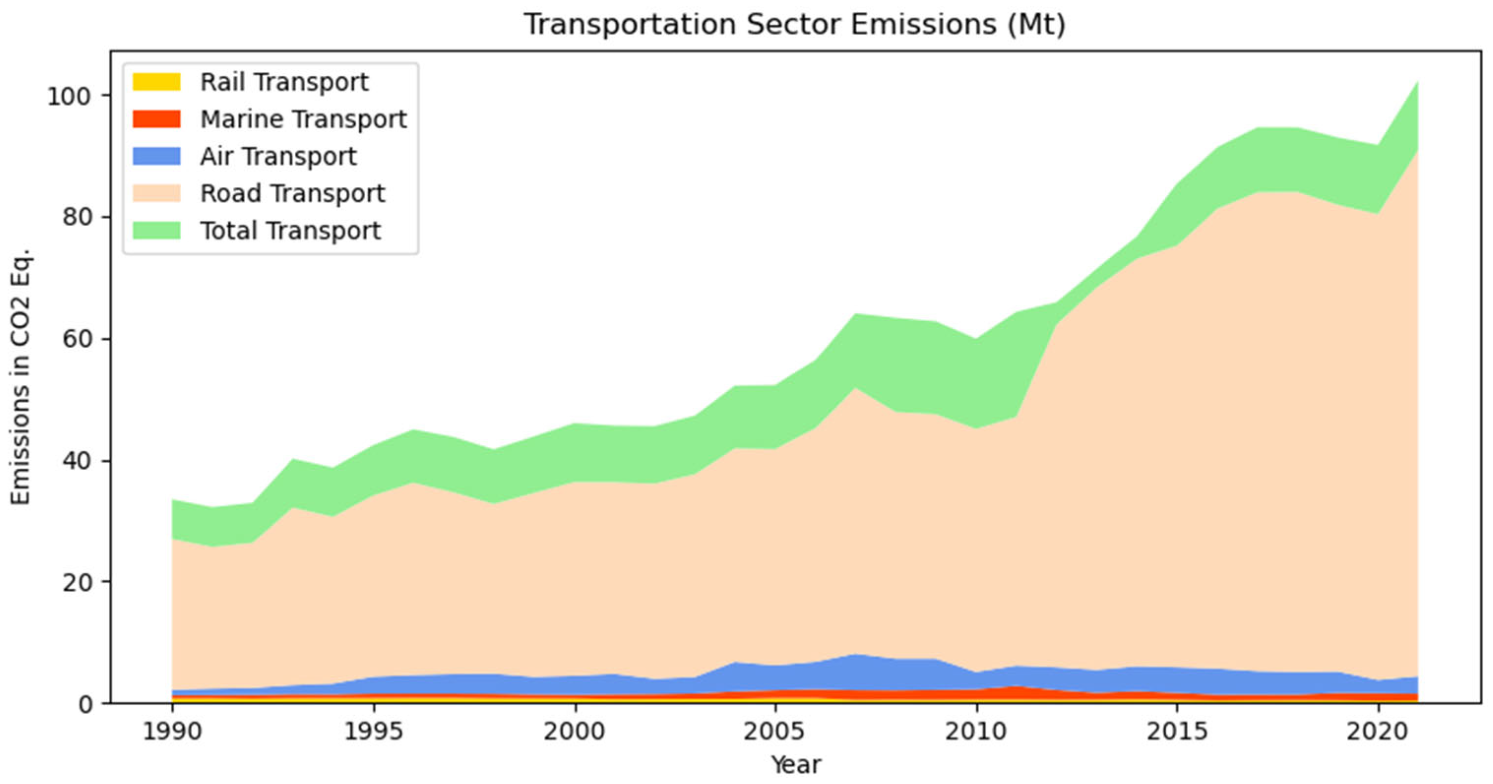
The data required to examine the case of Turkey were gathered from several sources for 1990–2021. Energy- and transportation-related inputs and the total and mode-based transportation emission outputs were obtained from TurkStat, Ministry of Environment, Urbanization and Climate Change and General Directorate of Highways in Turkey. Data on socioeconomic inputs were collected from the World Bank. Turkey’s total and mode-based transportation emissions in CO2 eq. from 1990 to 2021 are presented in Figure 2. The total transportation emissions include emissions originating from road, air, marine, and rail transport and other transport purposes (e.g., forestry, fisheries). It can clearly be seen that road transport accounts for a large portion of the total transport emissions over the years. In 2021, 94.8%, 3.1%, 1.2%, and 0.4% of transportation sector emissions originated from road, air, marine, and rail transport, respectively, with an additional 0.4% from other transport modes.

Figure 2.
The total and mode-based emissions in CO2 eq. originating from transportation.
4. Results and Discussion
Within the scope of the approach presented in this study, ridge regression, support vector machine, random forest, LSTM, and ANN models were applied to the case dataset of emissions from Turkey’s transportation systems. The models were built using Python 3.12.4. The dataset included the annual total and transportation mode-based emissions in CO2 eq. as a target (dependent) variable and a range of socioeconomic and energy- and transportation-related variables as predictors (independent variables). During data preprocessing, missing values were completed via interpolation and extrapolation. Correlation analysis was performed using Pearson correlation method to see the relationship between dependent and independent variables. Following the implementation of the correlation analysis, independent variables that demonstrated a moderate or higher level of relationship with the dependent variables were identified and selected to generate total, road, air, marine, and rail transport datasets. To adjust and scale the values of variables in the dataset, normalization was applied.
The dataset was partitioned into training and testing sets: 80% was used for training; and 20% was used for testing. Hyperparameter optimization was applied to tune the parameters of the employed models. The grid search technique, which is a comprehensive method of finding the best combination of hyperparameters, was used to tune the parameters of the models for each dataset.
4.1. Training and Testing Performance Results
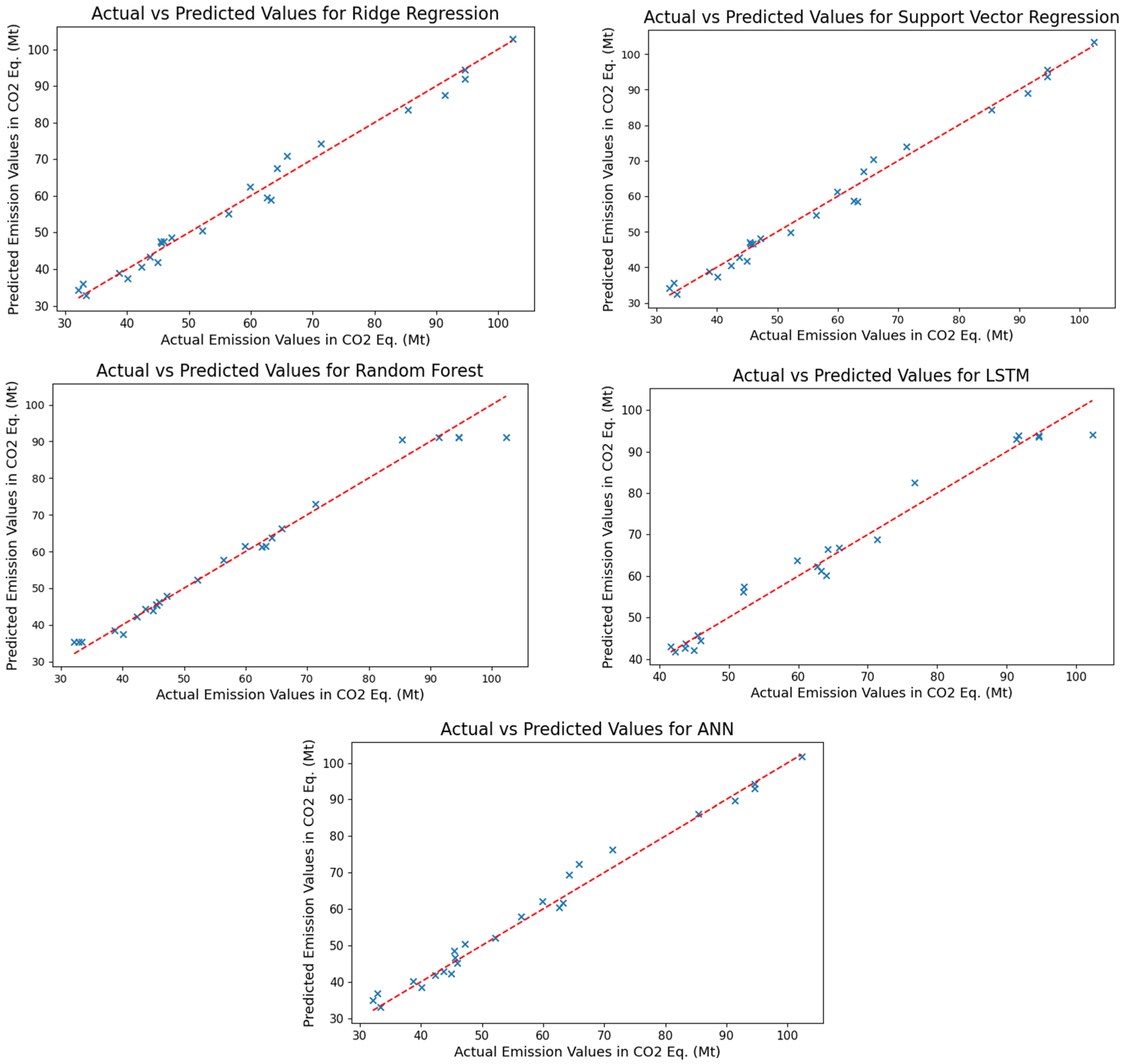
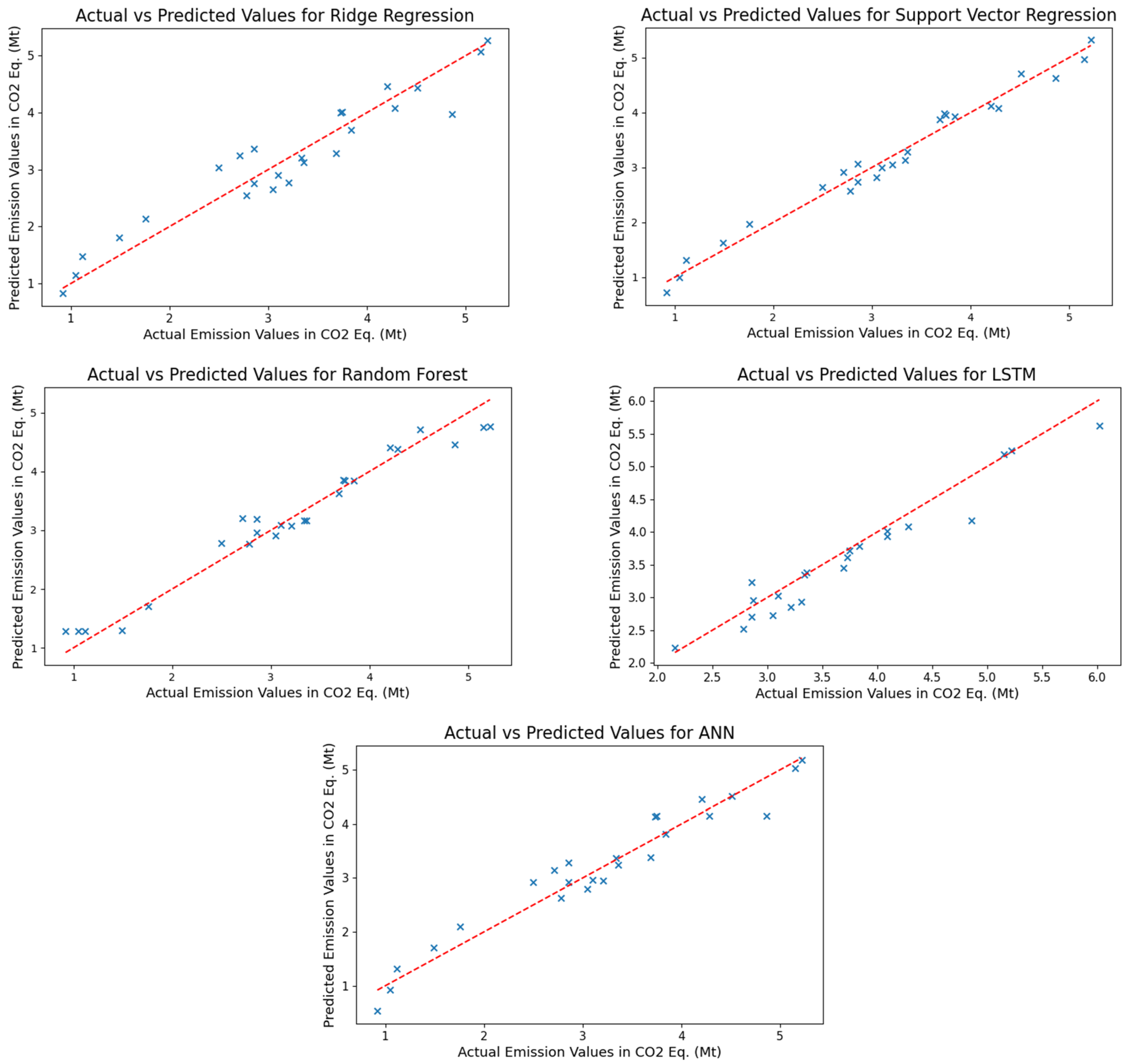
To evaluate performance of the adopted models on training datasets, actual emission values were compared with each model’s predicted values and visualized using actual vs. predicted value plots. The training results of the models for the total transport emissions in CO2 eq. are presented in Figure 3. Table 3 shows the performance results of the models for the total transport emissions test data in CO2 eq.
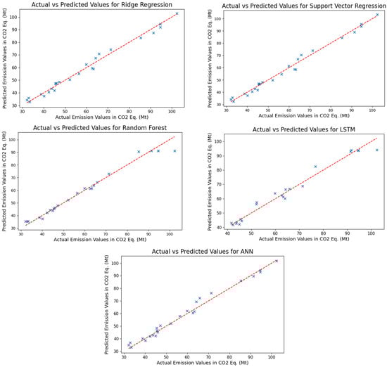
Figure 3.
Training results of algorithms for total transport emissions in CO2 eq.
Table 3.
Algorithm performance results for the total transport emissions test data in CO2 eq.
As demonstrated by the training results in relation to the total transport emissions, it can be observed that the predicted values obtained via the support vector regression algorithm show a high degree of proximity to the actual values. Furthermore, the ridge regression and ANN models exhibited better performance in comparison to the random forest and LSTM models. An examination of the results obtained from the models employed on the test dataset reveals that all models yielded values greater than 0.96, in terms of the R2 performance criterion. According to the MAPE performance criterion, it is apparent that all models demonstrate high prediction accuracy, as evidenced by the reference value ranges used by Lewis [42]. According to this MAPE classification, the forecasting accuracy is considered high for values less than or equal to 10%. For a range of 10–20%, accuracy is considered good; and for a range of 20–50%, accuracy is considered reasonable. Among the adopted algorithms, although its R2 values are identical to those of the support vector algorithm, the ANN achieved the best MAPE value. In the remaining performance measures, the support vector regression outperformed ANN.
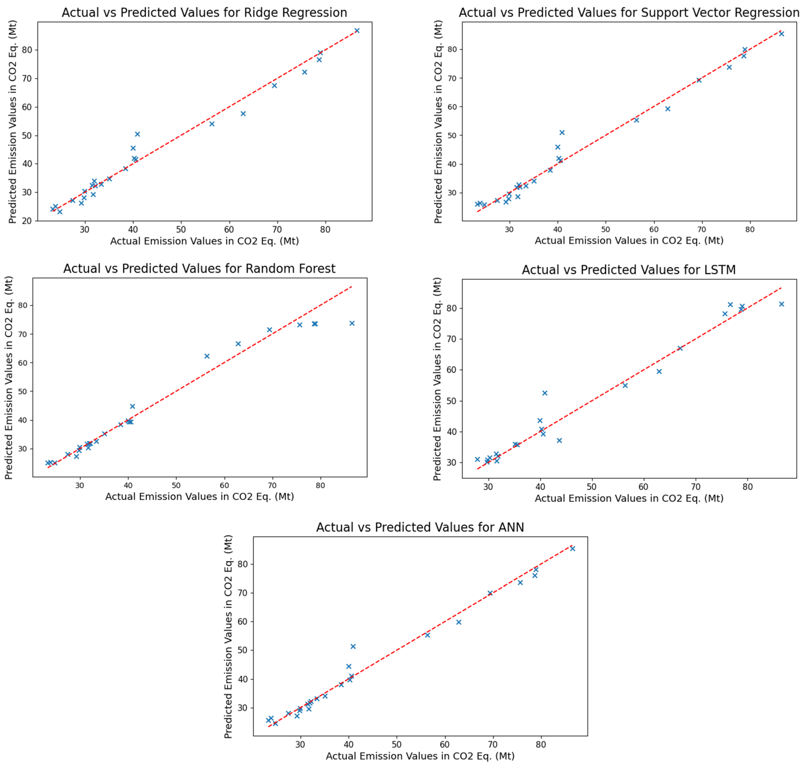
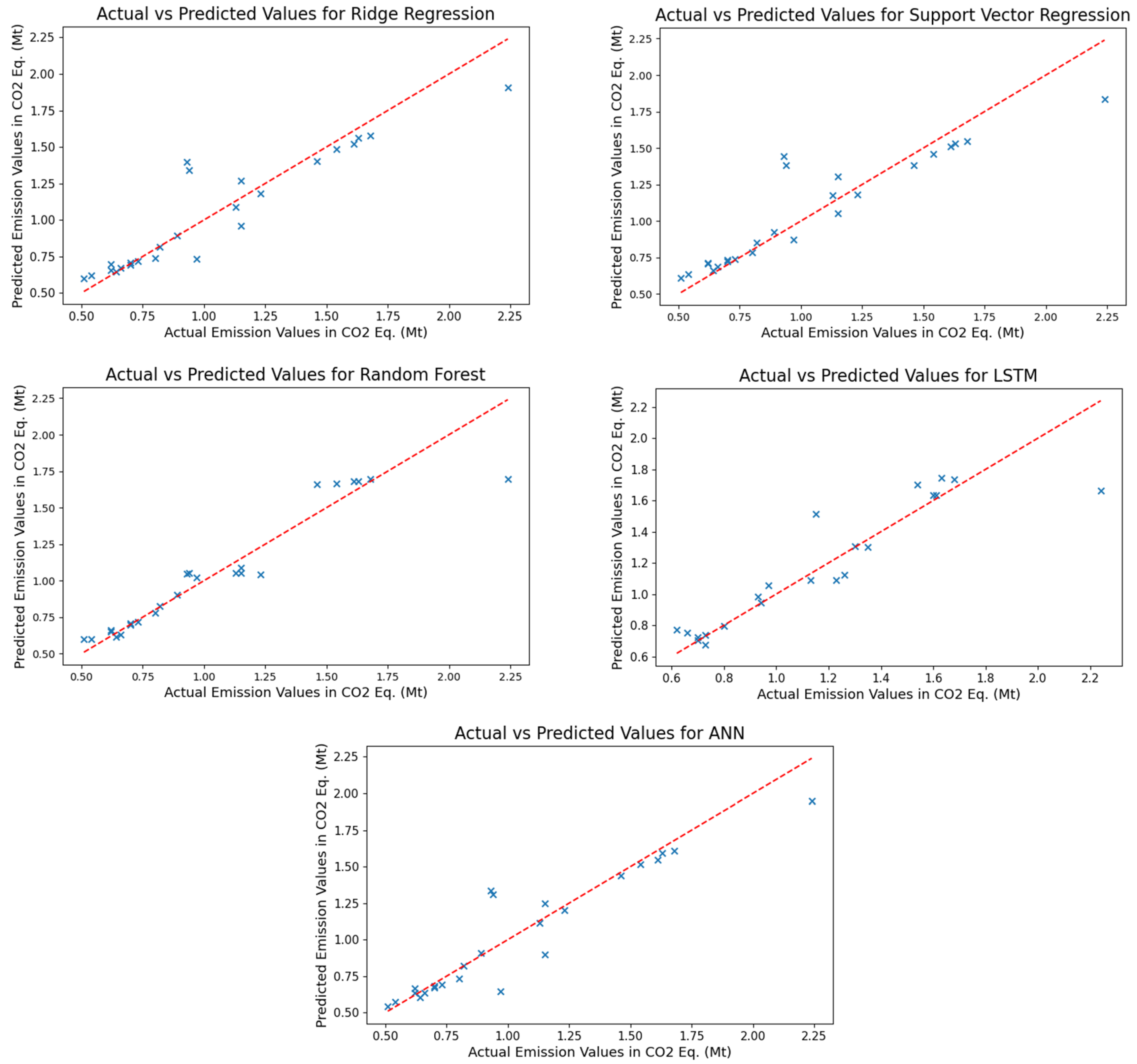
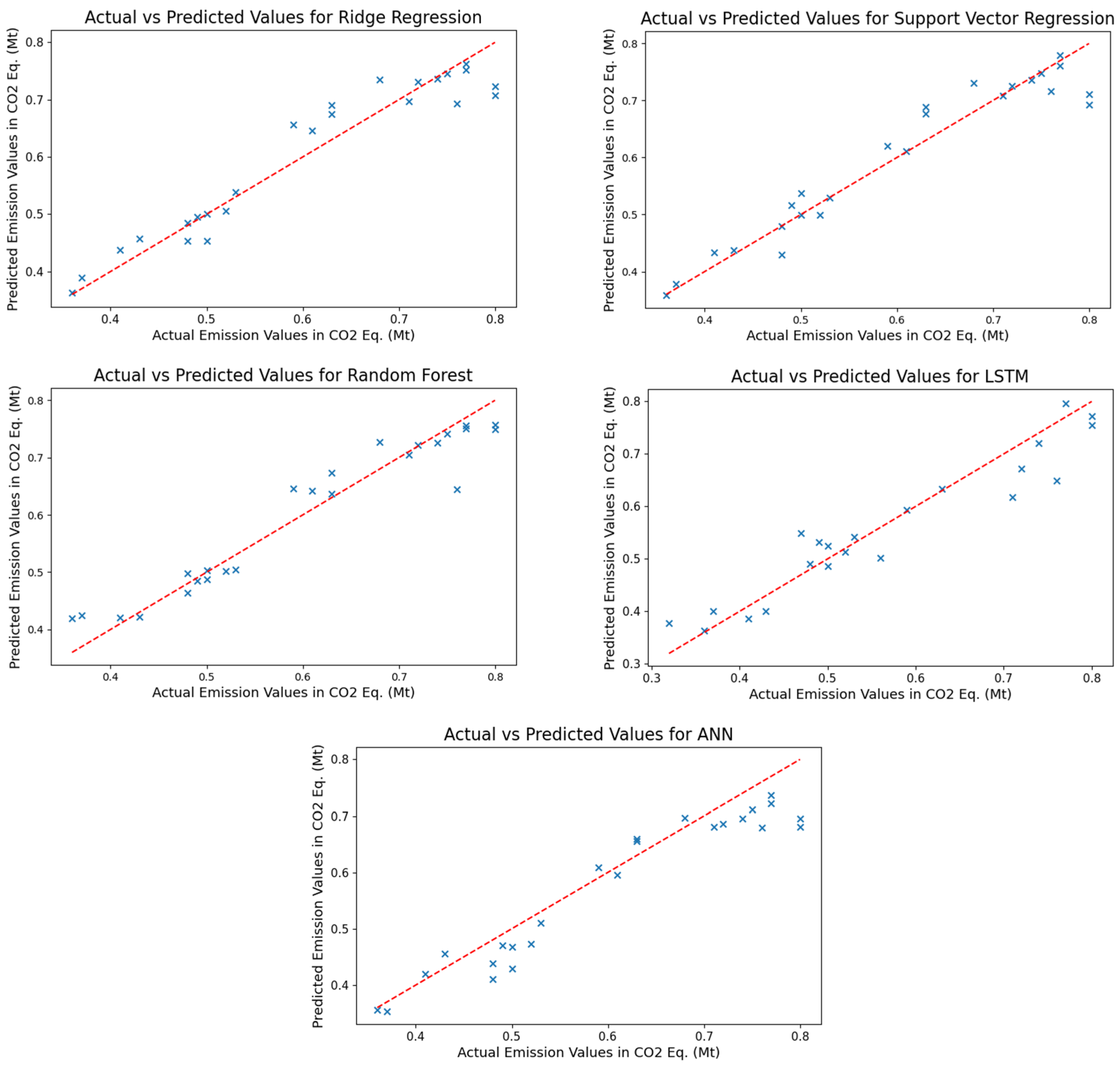
To draw conclusions regarding the contribution of distinct transportation modes to Turkey’s transport emissions in CO2 eq., analyses were conducted with datasets created for road, air, marine, and rail transport. The input and output variables employed in these datasets can be found in Table 2. The training results of the proposed algorithms for the road, air, marine, and rail transport emissions in CO2 eq. are provided in Figure 4, Figure 5, Figure 6 and Figure 7, respectively. Table 4, Table 5, Table 6 and Table 7 present performance results of the proposed algorithms for the road, air, marine, and rail transport emissions in CO2 eq.
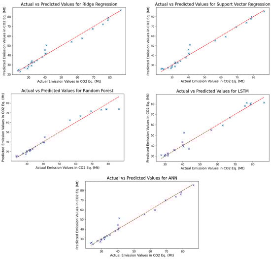
Figure 4.
Training results of algorithms for the road transport emissions in CO2 eq.
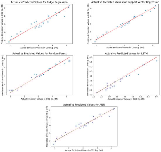
Figure 5.
Training results of algorithms for the air transport emissions in CO2 eq.
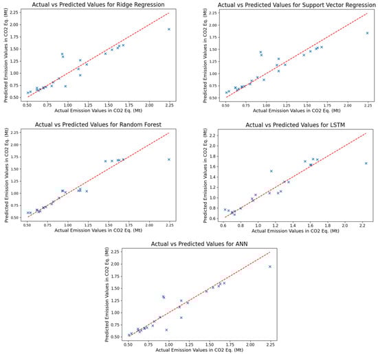
Figure 6.
Training results of algorithms for marine transport emissions in CO2 eq.
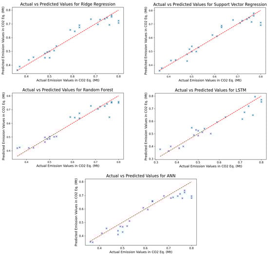
Figure 7.
Training results of algorithms for rail transport emissions in CO2 eq.
Table 4.
Algorithm performance results for road transport emissions test data in CO2 eq.
Table 5.
Algorithm performance results for air transport emissions test data in CO2 eq.
Table 6.
Algorithm performance results for marine transport emissions test data in CO2 eq.
Table 7.
Algorithm performance results for rail transport emissions test data in CO2 eq.
Based on the performance results of the models shown in Table 4 for the road transport emissions test data in CO2 eq., it can be observed that the support vector machine and random forest models emerge as the top-performing models with the lowest MSE, MAE, and RMSE performance metrics and highest R2 values. Nevertheless, ridge regression provides a balanced performance, with slightly higher error metrics but a strong R2 value. In terms of the MAPE performance measure, all models achieved high prediction accuracy.
An examination of the results of the air transport emissions test data in CO2 eq. was conducted which is shown in Table 5, revealing that the support vector machine model exhibited superior performance across all performance metrics when compared to the other models, with ridge regression ranking second. The ANN provides intermediate performance, outperforming the random forest and LSTM models but underperforming compared to the support vector machine and ridge regression models. The random forest provides good prediction accuracy in terms of the MAPE performance metric, while LSTM demonstrates inadequate performance for this dataset, exhibiting significantly larger errors and considerably lower R2 values when compared with the other models.
According to the findings of the performance results related to marine transport emissions test data in CO2 eq. shown in Table 6, the ANN provides the most accurate predictions, as reflected by the lowest MSE, MAE, RMSE, and MAPE values, along with the highest R2 value. LSTM also performs slightly below the ANN in terms of the MSE, MAE, RMSE, and R2 values. The second lowest MAPE value was attained by the ridge regression model.
The performance results shown in Table 7 for the rail transport emissions test data in CO2 eq. demonstrate that the support vector machine model achieved the highest R2 value. Despite an R2 value of 0.751, the LSTM network achieved the lowest MAPE value and exhibited high prediction accuracy. The remaining models exhibit good prediction accuracy in terms of the MAPE metric.
As a result, it can be interpreted that the support vector machine model is the most consistent and reliable across multiple transport systems, offering a balance of low error metrics and high R2 values. The ability of the support vector machine to generalize smaller datasets and its power to handle nonlinear relationships enable it to perform better. Furthermore, the combination of the epsilon loss function and the regularization mechanism makes support vector machines robust to overfitting. The use of LSTM and the ANN is contingent on specific requirements, such as the minimization of the MAPE or the management of more complex temporal dependencies. LSTMs minimize errors during training, particularly when dealing with sequential data, by retaining important information through memory cells, capturing long-term dependencies, and reducing the vanishing gradient problem. An ANN is also a powerful tool for reducing prediction errors and improving the accuracy of models by adjusting weights during training and using regularization techniques. Random forest and ridge regression techniques may be considered when simpler models are desired. The random forest algorithm is robust and highly accurate and works well for both small and large datasets. It handles noise and is easy to use with minimal tuning. Ridge regression offers a simple yet powerful means of regularizing the model to handle overfitting, making it more robust for real-world predictive tasks. Each model has its own strengths, but they also come with certain disadvantages. All are sensitive to data quality and hyperparameters. They require hyperparameter tuning, which can be time-consuming. Additionally, support vector machines, LSTM, and ANNs in particular are computationally expensive to train.
It is essential for policymakers to acknowledge that performance metrics can serve as instruments to assess the reliability of models’ predictions for decision-making processes. Furthermore, the efficacy of models is contingent on the quality of the data used. Real-world systems are complex and challenging to predict with absolute precision, even for the best models. The enhancement of performance metrics is an ongoing procedure, and data patterns can change over time (e.g., due to new policies or technologies). As new data are collected, models should be periodically updated and retrained to incorporate recent data and reflect changes. This may lead to better decision-making in the future and an improvement in model performance.
4.2. Future Projections Through Scenario Analysis
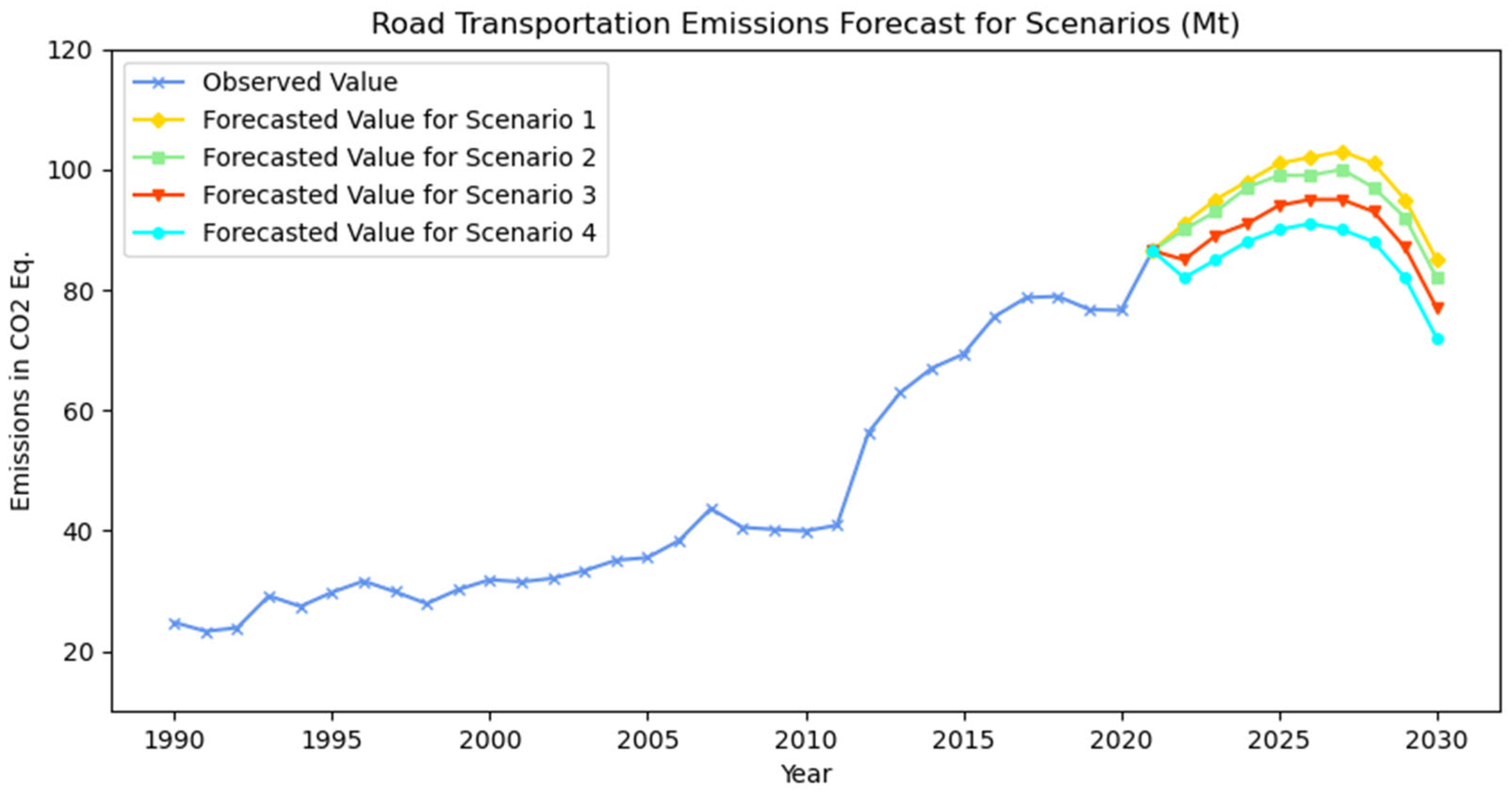
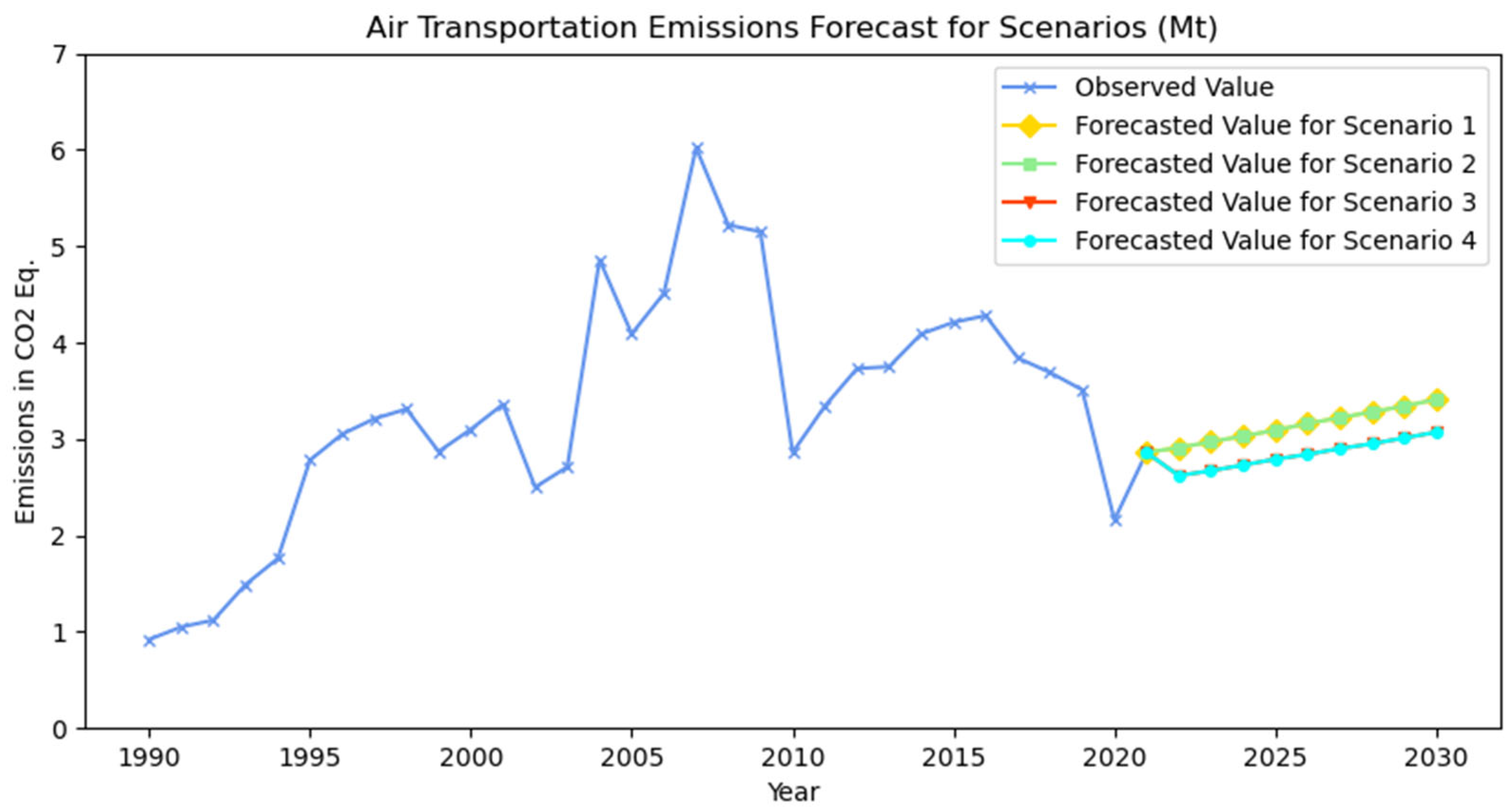
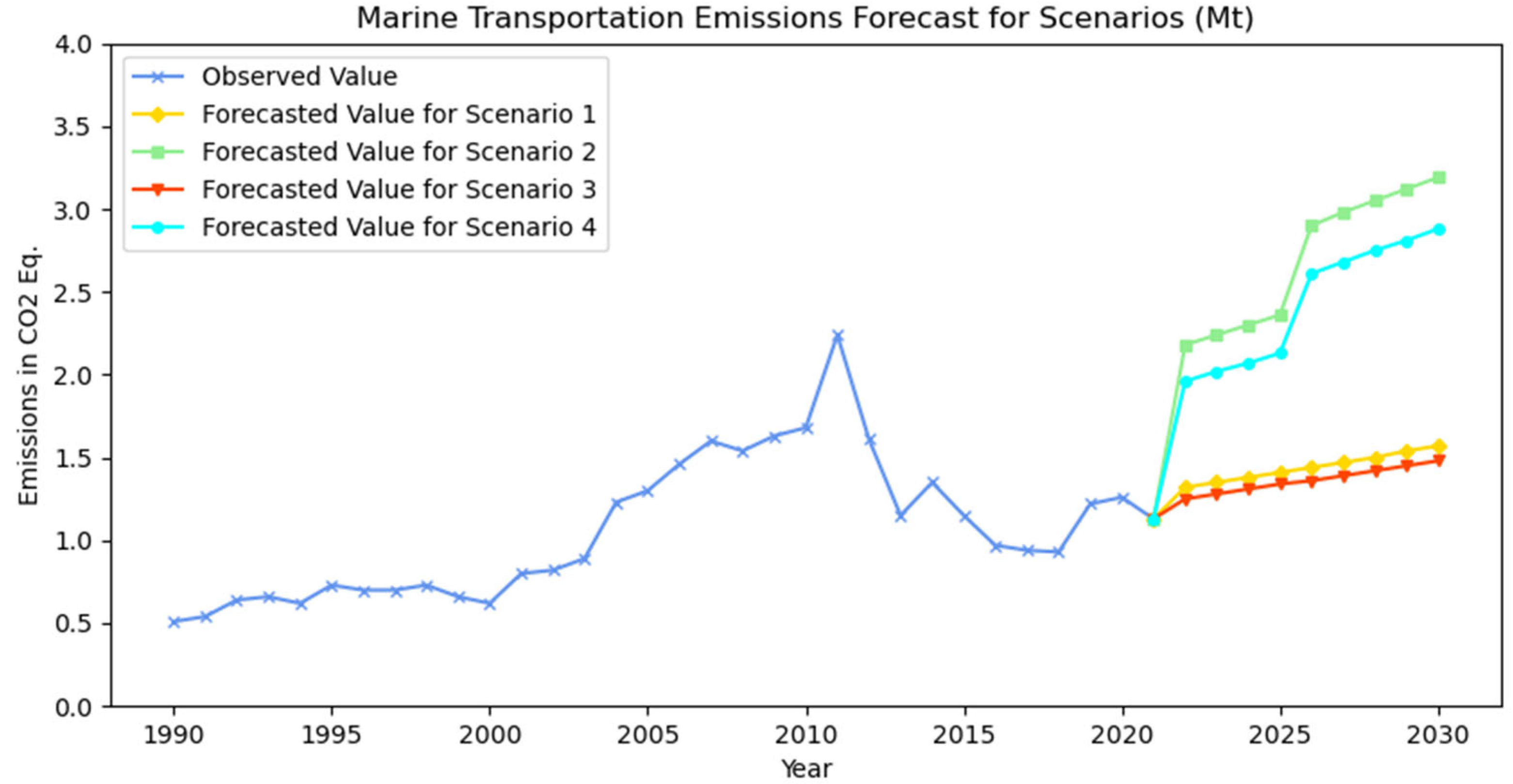
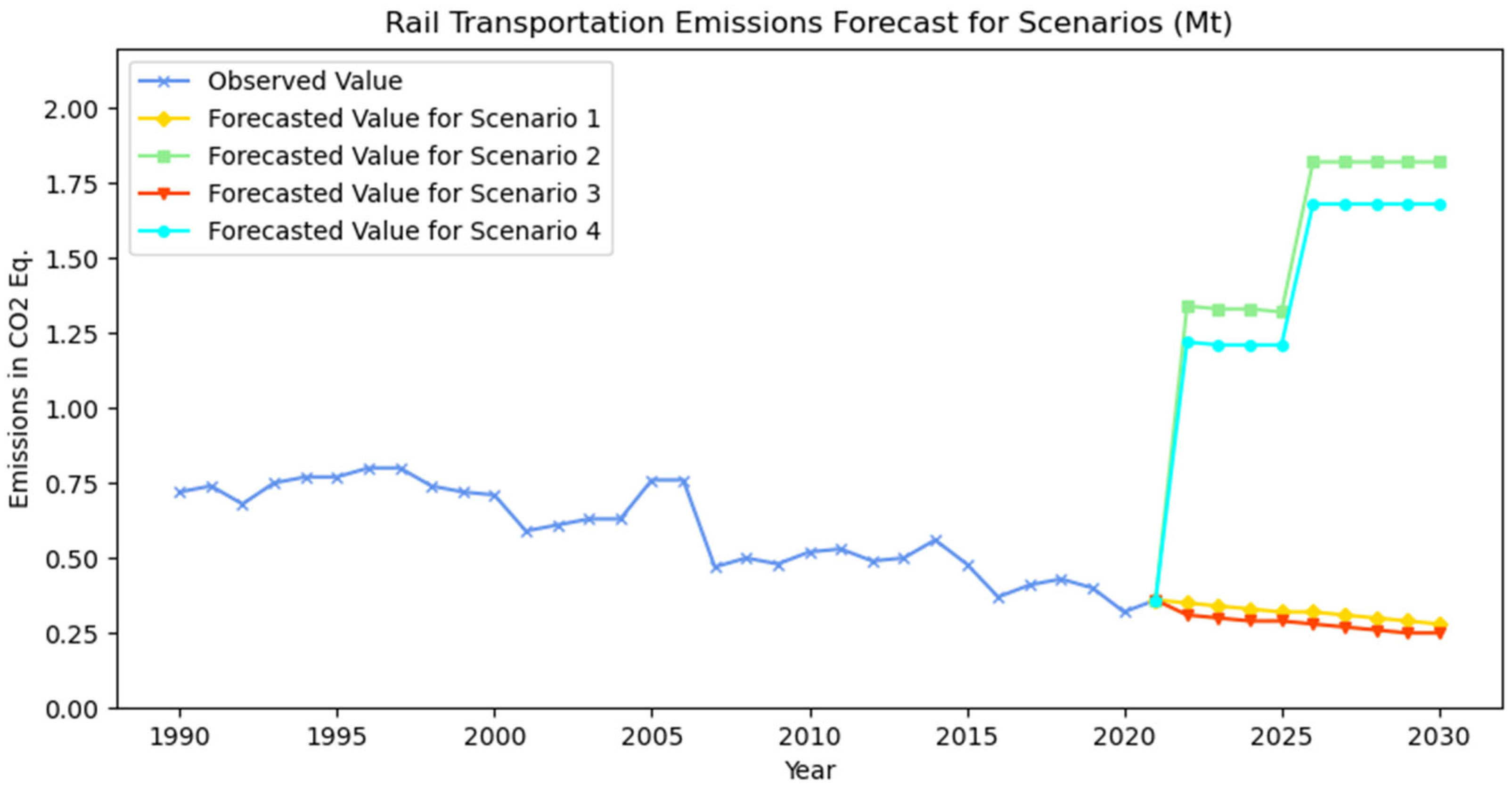
The 2024–2030 Climate Change Mitigation Strategy and Action Plan of the Ministry of Environment, Urbanisation and Climate Change of the Republic of Turkey [5] establishes sectoral strategies and actions. Accordingly, the following strategies have been defined for the transport sector: the promotion of a modal shift to marine/rail transportation, the enhancement of transport sector efficiency, the utilization of sustainable/clean energy sources in transport systems, and the undertaking of infrastructure activities deemed necessary for the decarbonization of the sector. In order to make future projections for transportation-related emissions, four scenarios have been defined, taking into consideration the emission mitigation strategies of the ministry. Scenario 1 is regarded as the baseline scenario, and it is hypothesized that the input parameters for each transport mode will demonstrate a similar trend to those observed in the past. In Scenario 1, future values of the input parameters are estimated based on their past values, using the exponential smoothing method. In Scenario 2, a gradual modal shift from road to marine and rail transport of up to 2% is assumed. Scenario 3 focuses on analyzing energy efficiency across all modes of transport. It is assumed that in Scenario 3, although the input parameters will show an increasing trend similar to that observed in the past, energy efficiency (when energy savings between 10% to 20% are reached) will be achieved for all modes of transport. Finally, Scenario 4 represents a combination of a gradual shift to marine and rail transport, as defined in Scenario 2, and the achievement of energy efficiency in all transport modes, as described in Scenario 3. The development of scenarios concerning the utilization of sustainable and clean energy sources in transport systems, in addition to the infrastructure strategies necessary for the decarbonization of the sector, was not possible due to a lack of data. The future projection results for the road, air, marine, and rail transportation modes for defined scenarios in terms of CO2 eq. are presented in Figure 8, Figure 9, Figure 10 and Figure 11, respectively.
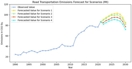
Figure 8.
Future projections for road transportation.
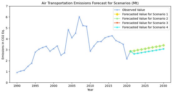
Figure 9.
Future projections for air transportation.

Figure 10.
Future projections for marine transportation.
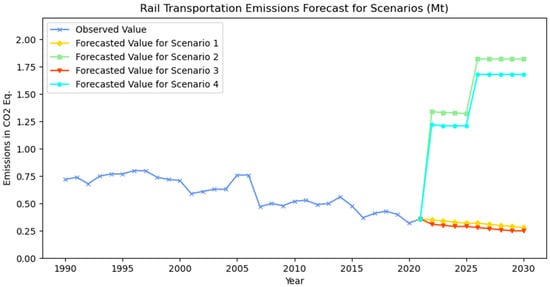
Figure 11.
Future projections for rail transportation.
When the future forecast results for road transport are analyzed, it is observed that in Scenario 1, the amount of emissions shows an increasing trend at first, followed by a decreasing trend due to the foreseen widespread use of electric and hybrid vehicle technologies. In Scenario 2, a decrease in emissions is observed compared to Scenario 1 with the conditions of a gradual transition to marine and railway transportation. In Scenario 3, the decrease relative to Scenario 1 continues as improvements in the amount of energy consumed occur due to increasing energy efficiency. In Scenario 4, a significant downward trend in the amount of emissions is observed.
While there is an increasing trend in air transport emissions under Scenario 1, Scenario 2 demonstrates a similar emissions level to Scenario 1, showing no significant further increases or reductions. In Scenario 3, a decrease in the rate of increase in emissions is observed with the projected decrease in the amount of energy consumed. The results of Scenario 4 are similar to those of Scenario 3. Compared to other transport modes, constraints in reducing aviation emissions reflect the difficulty of decarbonizing air transport.
Based on findings of future projections of marine transport, a slight increase in emissions from marine transport is observed in Scenario 1; conversely, a significant increase in emissions is observed when the modal shift from road transport is considered in Scenario 2. A decline in the rate of increase in emissions is evident upon considering the decrease in energy consumption in Scenario 3; nevertheless, a marked upward trend emerges in Scenario 4 in conjunction with that of Scenario 2. It should be noted that the increase in Scenarios 2 and 4 is significantly more minimal in comparison to the potential increase in the case of road transportation.
According to future projections for the rail transport, in Scenarios 2 and 4, an increase similar to that observed in the case of marine transport is predicted, while a slight decrease in emissions is expected in Scenarios 1 and 3, in line with previous trends and energy efficiency.
Consequently, analyses were conducted to ascertain Turkey’s climate change dynamics, with the scenarios developed in accordance with the climate change action plan. The potential impact of policy decisions and technological advancements on reducing the CO2 emissions of the transportation system were discussed. The most fundamental policy for reducing transport sector emissions was a modal shift towards marine and rail transport, which are more efficient in terms of both energy use and emissions per unit of mobility (tonne-km and passenger-km). In order to achieve this modal shift, it is important to provide services that compete with road and/or air transport services in both rail and maritime transport services, with supporting infrastructure in marine and railway transport, encouraging intermodal and combined transport in freight transport. Increasing energy efficiency in transport systems is another critical policy to reduce CO2 emissions. For this purpose, the most prominent actions are making private and shared transport more efficient and encouraging the use of public transport systems and new-generation low- or zero-emission vehicles.
Although scenario analysis provides a comprehensive approach to managing uncertainties and improving strategic planning, it should be also noted that this study has some limitations. The impact of macroeconomic variables, like fluctuations in fuel prices and changes in inflation, the behavioral uncertainty of consumers, and uncertainties or insufficiencies in historical data such as the use of clean energy sources in transport systems and infrastructure strategies, introduce significant challenges. These limitations may affect the accuracy of the predictions, and assumptions may not capture the full range of possible future outcomes. To mitigate these uncertainties, integrating expert judgment into the analysis or conducting a sensitivity analysis could help provide a more informed perspective.
5. Conclusions
Climate change represents a major environmental challenge for the contemporary world. The present study investigated emissions resulting from the transport system, which has been identified as one of the three top global contributors to climate change. This study contributes to the literature with a comprehensive approach for estimation of the emissions of transportation systems in CO2 eq., considering a range of socioeconomic and energy- and transportation-related input variables. The proposed approach incorporates ridge regression, support vector machine, random forest, LSTM, and ANN models. Using a dataset of Turkey, the adopted models were applied to the case of emissions from Turkey’s transportation system. This study employed a transportation type-based analysis to investigate the contributions of Turkey’s road, air, marine, and rail transportation systems through scenario analysis in line with the Climate Change Mitigation Strategy and Action Plan of the Ministry of Environment, Urbanisation, and Climate Change of the Republic of Turkey. To the best of the authors’ knowledge, there have been limited research efforts conducted on transportation type-based emissions analysis considering a range of input variables. It is evident from the findings of the present study that ANN, machine learning, and deep learning models have potential to be utilized for forecasting emissions data with a limited size, with the resultant forecasts demonstrating a satisfactory degree of accuracy.
Based on the results of this study, it can be suggested that ensuring energy efficiency in transport systems and a modal shift to marine and rail transport can result in significant reductions in transport emissions. To achieve this objective, a number of strategies can be proposed. These include the expansion of marine and rail transport infrastructure, the improvement of public transportation networks, and the integration of electric buses and trains into the public transport system. Further suggestions include financial incentives for the purchase of electric and hybrid vehicles, encouraging the development of renewable energy sources to provide clean electricity for electric vehicles, transitioning to sustainable fuels, public awareness campaigns, and research on new technologies to support low-carbon transportation, such as advanced battery storage.
Funding
This research received no external funding.
Data Availability Statement
The raw data supporting the conclusions of this article will be made. Available by the authors upon request.
Conflicts of Interest
The authors declare no conflicts of interest.
Abbreviations
The following abbreviations are used in this manuscript:
| GHG | Greenhouse Gas |
| NDC | Nationally Determined Contribution |
| UNFCCC | United Nations Framework Convention on Climate Change |
| TurkStat | Turkish Statistics Institute |
| EU | European Union |
| GDP | Gross Domestic Product |
| LSTM | Long Short-Term Memory |
| ANN | Artificial Neural Network |
| MSE | Mean Square Error |
| MAE | Mean Absolute Error |
| RMSE | Root Mean Square Error |
| MAPE | Mean Absolute Percentage Error |
| TRY | Turkish Lira |
| Ttoe | Thousand Tonnes of Oil Equivalent |
| Km | Kilometer |
| M | Million |
| Mt | Million Tonnes |
References
- Ho, W.T.; Yu, F.W. Optimal selection of predictors for greenhouse gas emissions forecast in Hong Kong. J. Clean. Prod. 2022, 370, 133310. [Google Scholar] [CrossRef]
- Marrakech Partnership. Climate Action Pathway: Transport, Vision and Summary; United Nations Climate Change: Bonn, Germany, 2021. [Google Scholar]
- International Energy Agency. CO2 Emissions in 2022; International Energy Agency: Paris, France, 2023. [Google Scholar]
- Marrakech Partnership. Climate Action Pathway: Transport, Vision and Summary; United Nations Climate Change: Bonn, Germany, 2020. [Google Scholar]
- T.C. Ministry of Environment, Urbanisation and Climate Change. Climate Change Mitigation Strategy and Action Plan (2024–2030); T.C. Ministry of Environment, Urbanisation and Climate Change: Ankara, Turkey, 2024.
- T.C. Ministry of Environment, Urbanisation and Climate Change. Environmental Indicators; T.C. Ministry of Environment, Urbanisation and Climate Change: Ankara, Turkey, 2023.
- Ene Yalçın, S. Development of A Forecasting Framework Based on Advanced Machine Learning Algorithms for Greenhouse Gas Emissions. Systems 2024, 12, 528. [Google Scholar] [CrossRef]
- Lu, J.; Lewis, C.; Lin, S.J. The forecast of motor vehicle, energy demand and CO2 emission from Taiwan’s road transportation sector. Energy Policy 2009, 37, 2952–2961. [Google Scholar] [CrossRef]
- Kazancoglu, Y.; Ozbiltekin-Pala, M.; Ozkan-Ozen, Y.D. Prediction and evaluation of greenhouse gas emissions for sustainable road transport within Europe. Sustain. Cities Soc. 2021, 70, 102924. [Google Scholar] [CrossRef]
- Huang, S.; Xiao, X.; Guo, H. A novel method for carbon emission forecasting based on EKC hypothesis and nonlinear multivariate grey model: Evidence from transportation sector. Environ. Sci. Pollut. Res. 2022, 29, 60687–60711. [Google Scholar] [CrossRef]
- Yagcitekin, B.; Uzunoglu, M.; Karakas, A.; Erdinc, O. Assessment of electrically-driven vehicles in terms of emission impacts and energy requirements: A case study for Istanbul, Turkey. J. Clean. Prod. 2015, 96, 486–492. [Google Scholar] [CrossRef]
- Li, X.; Ren, A.; Li, Q. Exploring Patterns of Transportation-Related CO2 Emissions Using Machine Learning Methods. Sustainability 2022, 14, 4588. [Google Scholar] [CrossRef]
- Abdulmalik, R.; Srivastava, G. Forecasting of Transportation-related CO2 Emissions in Canada with Different Machine Learning Algorithms. Adv. Artif. Intell. Mach. Learn. 2023, 3, 1295–1312. [Google Scholar] [CrossRef]
- Javanmard, M.E.; Tang, Y.; Wang, Z.; Tontiwachwuthikul, P. Forecast energy demand, CO2 emissions and energy resource impacts for the transportation sector. Appl. Energy 2023, 338, 120830. [Google Scholar] [CrossRef]
- Qiao, Q.; Eskandari, H.; Saadatmand, H.; Sahraei, M.A. An interpretable multi-stage forecasting framework for energy consumption and CO2 emissions for the transportation sector. Energy 2024, 286, 129499. [Google Scholar] [CrossRef]
- Temizceri, F.T.; Kara, S.S. Towards sustainable logistics in Turkey: A bi-objective approach to green intermodal freight transportation enhanced by machine learning. Res. Transp. Bus. Manag. 2024, 55, 101145. [Google Scholar] [CrossRef]
- Çınarer, G.; Yeşilyurt, M.K.; Ağbulut, Ü.; Zeki Yılbaşı, Z.; Kılıç, K. Application of various machine learning algorithms in view of predicting the CO2 emissions in the transportation sector. Sci. Tech. Energ. Transit. 2024, 79, 15. [Google Scholar] [CrossRef]
- Ratanavaraha, V.; Jomnonkwao, S. Trends in Thailand CO2 emissions in the transportation sector and Policy Mitigation. Transp. Policy 2015, 41, 136–146. [Google Scholar] [CrossRef]
- Alhindawi, R.; Abu Nahleh, Y.; Kumar, A.; Shiwakoti, N. Projection of Greenhouse Gas Emissions for the Road Transport Sector Based on Multivariate Regression and the Double Exponential Smoothing Model. Sustainability 2020, 12, 9152. [Google Scholar] [CrossRef]
- Isik, M.; Sarica, K.; Ari, I. Driving forces of Turkey’s transportation sector CO2 emissions: An LMDI approach. Transp. Policy 2020, 97, 210–219. [Google Scholar] [CrossRef]
- Lu, Q.; Chai, J.; Wang, S.; Zhang, Z.G.; Sun, X.C. Potential energy conservation and CO2 emissions reduction related to China’s road transportation. J. Clean. Prod. 2020, 245, 118892. [Google Scholar] [CrossRef]
- Zhu, L.; Li, Z.; Yang, X.; Zhang, Y.; Li, H. Forecast of Transportation CO2 Emissions in Shanghai under Multiple Scenarios. Sustainability 2022, 14, 13650. [Google Scholar] [CrossRef]
- Chang, C.-C.; Chang, K.-C.; Lin, Y.-L. Policies for reducing the greenhouse gas emissions generated by the road transportation sector in Taiwan. Energy Policy 2024, 191, 114171. [Google Scholar] [CrossRef]
- Rajan, M.P. An Efficient Ridge Regression Algorithm with Parameter Estimation for Data Analysis in Machine Learning. SN Comput. Sci. 2022, 3, 171. [Google Scholar] [CrossRef]
- Höfler, L. Good results from sensor data: Performance of machine learning algorithms for regression problems in chemical sensors. Sensor Actuat. B Chem. 2024, 421, 136528. [Google Scholar] [CrossRef]
- Ge, X.; Xu, F.; Wang, Y.; Li, H.; Wang, F.; Hu, J.; Li, K.; Xiaoxing Lu, X.; Chen, B. Spatio-Temporal Two-Dimensions Data Based Customer Baseline Load Estimation Approach Using LASSO Regression. IEEE Trans. Ind. Appl. 2022, 58, 3112–3122. [Google Scholar] [CrossRef]
- Lin, G.; Lin, A.; Gu, D. Using support vector regression and K-nearest neighbors for short-term traffic flow prediction based on maximal information coefficient. Inf. Sci. 2022, 608, 517–531. [Google Scholar] [CrossRef]
- Wen, L.; Cao, Y. Influencing factors analysis and forecasting of residential energy related CO2 emissions utilizing optimized support vector machine. J. Clean. Prod. 2020, 250, 119492. [Google Scholar] [CrossRef]
- Wang, C.; Lia, M.; Yan, J. Forecasting carbon dioxide emissions: Application of a novel two-stage procedure based on machine learning models. J. Water Clim. Change 2023, 14, 477–493. [Google Scholar] [CrossRef]
- Li, Y.; Zou, C.; Berecibar, M.; Nanini-Maury, E.; Chan, J.C.-W.; Bossche, P.; Mierlo, J.V.; Omar, N. Random forest regression for online capacity estimation of lithium-ion batteries. Appl. Energy 2018, 232, 197–210. [Google Scholar] [CrossRef]
- Vukovic, D.B.; Spitsina, L.; Gribanova, E.; Spitsin, V.; Lyzin, I. Predicting the Performance of Retail Market Firms: Regression and Machine Learning Methods. Mathematics 2023, 11, 1916. [Google Scholar] [CrossRef]
- Zhou, Z.-H. Machine Learning; Springer: Singapore, 2021. [Google Scholar]
- Hasan, M.W. Design of an IoT model for forecasting energy consumption of residential buildings based on improved long short-term memory (LSTM). Meas. Energy 2025, 5, 100033. [Google Scholar] [CrossRef]
- Stefenon, S.F.; Seman, L.O.; Silva, E.C.; Finardi, E.C.; Coelho, L.S.; Mariani, V.C. Hypertuned wavelet convolutional neural network with long short-term memory for time series forecasting in hydroelectric power plants. Energy 2024, 313, 133918. [Google Scholar] [CrossRef]
- Kalteh, A.M. Monthly river flow forecasting using artificial neural network and support vector regression models coupled with wavelet transform. Comput. Geosci. 2013, 54, 1–8. [Google Scholar] [CrossRef]
- Rivero-Cacho, A.; Sanchez-Barroso, G.; Gonzalez-Dominguez, J.; Garcia-Sanz-Calcedo, J. Long-term power forecasting of photovoltaic plants using artificial neural networks. Energy Rep. 2024, 12, 2855–2864. [Google Scholar] [CrossRef]
- Ali, M.; Nayahi, J.V.; Abdi, E.; Ghorbani, M.A.; Mohajeri, F.; Farooque, A.A.; Alamery, S. Improving daily reference evapotranspiration forecasts: Designing AI-enabled recurrent neural networks based long short-term memory. Ecol. Inform. 2025, 85, 102995. [Google Scholar] [CrossRef]
- Sahin, B.; Canpolat, C.; Bilgili, M. Flow data forecasting for the junction flow using artificial neural network. Flow Meas. Instrum. 2024, 100, 102703. [Google Scholar] [CrossRef]
- Pramanik, P.; Jana, R.K.; Ghosh, I. AI readiness enablers in developed and developing economies: Findings from the XGBoost regression and explainable AI framework. Technol. Forecast. Soc. Change 2024, 205, 123482. [Google Scholar] [CrossRef]
- Akyol, M.; Uçar, E. Carbon footprint forecasting using time series data mining methods: The case of Turkey. Environ. Sci. Pollut. Res. 2021, 28, 38552–38562. [Google Scholar] [CrossRef]
- Kayakuş, M.; Terzioğlu, M.; Erdoğan, D.; Zetter, S.A.; Kabas, O.; Moiceanu, G. European Union 2030 Carbon Emission Target: The Case of Turkey. Sustainability 2023, 15, 13025. [Google Scholar] [CrossRef]
- Lewis, C.D. Industrial and Business Forecasting Methods; Butterworths-Heinemann: London, UK, 1982. [Google Scholar]

Disclaimer/Publisher’s Note: The statements, opinions and data contained in all publications are solely those of the individual author(s) and contributor(s) and not of MDPI and/or the editor(s). MDPI and/or the editor(s) disclaim responsibility for any injury to people or property resulting from any ideas, methods, instructions or products referred to in the content. |
© 2025 by the author. Licensee MDPI, Basel, Switzerland. This article is an open access article distributed under the terms and conditions of the Creative Commons Attribution (CC BY) license (https://creativecommons.org/licenses/by/4.0/).